Variational problems with long-range interaction
Nicola Soave, Hugo Tavares, Susanna Terracini, Alessandro, Zilio

TL;DR
This paper studies variational problems involving densities that repel each other at a distance, focusing on regularity, free-boundary conditions, and initial boundary behavior analysis.
Contribution
It introduces a framework for analyzing densities with long-range repulsion, establishing regularity results, free-boundary conditions, and preliminary characterizations of the free boundary.
Findings
Established regularity properties of solutions.
Proved a free-boundary condition for the problem.
Provided initial characterizations of the free boundary.
Abstract
We consider a class of variational problems for densities that repel each other at distance. Typical examples are given by the Dirichlet functional and the Rayleigh functional \[ D(\mathbf{u}) = \sum_{i=1}^k \int_{\Omega} |\nabla u_i|^2 \quad \text{or} \quad R(\mathbf{u}) = \sum_{i=1}^k \frac{\int_{\Omega} |\nabla u_i|^2}{\int_{\Omega} u_i^2} \] minimized in the class of functions attaining some boundary conditions on , and subjected to the constraint \[ \mathrm{dist} (\{u_i > 0\}, \{u_j > 0\}) \ge 1 \qquad \forall i \neq j. \] For these problems, we investigate the optimal regularity of the solutions, prove a free-boundary condition, and derive some preliminary results characterizing the free boundary .
Click any figure to enlarge with its caption.
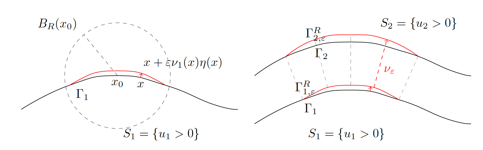 Figure 1
Peer Reviews
No public reviews on file for this paper yet. If you reviewed it on a platform where reviews are public (OpenReview, ICLR, NeurIPS, ICML), you can paste yours below so the community can read it here.
Videos
No videos yet. Explain this paper in a talk, walkthrough, or lecture? Add one.
Variational problems with long-range interaction
Nicola Soave
Nicola Soave
Dipartimento di Matematica, Politecnico di Milano,
Via Edoardo Bonardi 9, 20133 Milano, Italy
[email protected]; [email protected]
,
Hugo Tavares
Hugo Tavares
CAMGSD (Center for Mathematical Analysis, Geometry and Dynamical Systems)
Departamento de Matemática, Instituto Superior Técnico, Universidade de Lisboa
Av. Rovisco Pais, 1049-001 Lisboa, Portugal
and
Departamento de Matemática, Faculdade de Ciências da Universidade de Lisboa
Edifício C6, Piso 1, Campo Grande 1749-016 Lisboa, Portugal
[email protected]; [email protected]
,
Susanna Terracini
Susanna Terracini
Dipartimento di Matematica “Giuseppe Peano”, Università di Torino,
Via Carlo Alberto, 10, 10123 Torino, Italy
and
Alessandro Zilio
Alessandro Zilio
École des Hautes Études en Sciences Sociales, PSL Research University Paris, Centre d’analyse et de mathématique sociales (CAMS), CNRS,
190-198 Avenue de France, 75244, Paris CEDEX 13, France
[email protected], [email protected]
Abstract.
We consider a class of variational problems for densities that repel each other at distance. Typical examples are given by the Dirichlet functional and the Rayleigh functional
[TABLE]
minimized in the class of functions attaining some boundary conditions on , and subjected to the constraint
[TABLE]
For these problems, we investigate the optimal regularity of the solutions, prove a free-boundary condition, and derive some preliminary results characterizing the free boundary .
Key words and phrases:
Free boundary condition, Lipschitz regularity, Long-range interaction, Optimal partition problems, Segregation problems, Variational methods
1. Introduction
The object of this paper is the study of a class of minimal configurations for variational problems involving arbitrarily many densities related by long-range repulsive interactions. The mathematical setting we consider is described by the following two archetypical situations.
Problem (A) Let be a bounded domain of , , and let
[TABLE]
Given nonnegative nontrivial functions satisfying 111Here and in the rest of the paper, the distance between two sets and is understood as
(1.1)
[TABLE]
we consider the minimization problem
[TABLE]
where the set and the functional are defined by
[TABLE]
and
[TABLE]
The support of each component is taken in the weak sense: it corresponds to the complement in of the largest open set where a.e. on (cf. [3, Proposition 4.17]). Notice also that the existence of with the above properties imposes some conditions on (for instance, the diameter of cannot be too small), and we suppose that such conditions are satisfied.
We are interested in existence and qualitative properties of minimizers.
Problem (B) Let be a bounded domain of , , and let . We consider the set of open partitions of at distance , defined as
[TABLE]
Then, for a cost function satisfying
- •
for all and , which in particular yields that is component-wise increasing;
- •
for any given ,
[TABLE]
for all ,
we consider the minimization problem
[TABLE]
where is the first eigenvalue of the Laplace operator in with homogeneous Dirichlet boundary conditions. Problem (1.4) is a particular case of an optimal partition problem (cf. [1, 4]). A typical case we have in mind is the cost function .
We are interested in existence and qualitative properties of an optimal partition.
Our main results are, for problem (A):
- •
the existence of a minimizer;
- •
the optimal interior regularity of any minimizer;
- •
the derivation of several properties of the positivity sets ;
- •
the derivation of a free boundary condition involving the normal derivatives of different components of any minimizers on the regular part of the free-boundary .
For problem (B):
- •
the introduction of a weak formulation in terms of densities, and the existence of weak solutions;
- •
the global optimal regularity of any weak solution, which leads in particular to the existence of a strong solution for the original problem;
- •
the derivation of properties of the subsets , and of a free boundary condition on the regular part of .
In a forthcoming paper, we will study more in detail the regularity of the free-boundary.
We stress that, both in problems (A) and (B), the interaction among different densities takes place at distance: in problem (A) the positivity sets , and in problem (B) the open subsets , are indeed forced to stay at a fixed minimal distance from each other.
When the interaction among the densities takes place point-wisely, segregation problems analogue to (A) and (B) have been studied intensively, in connection with optimal partition problems for Laplacian eigenvalues [9, 10, 11, 5, 21, 26, 25], with the regularity theory of harmonic maps into singular manifold [6, 12, 25], and with segregation phenomena for systems of elliptic equations arising in quantum mechanics driven by strong competition [6, 13, 18, 22, 23, 24, 30].
In contrast, the only results available so far regarding segregation problems driven by long-range competition are given in [7], where the authors analyze the spatial segregation for systems of type
[TABLE]
with . In the above equation, denotes the characteristic function of , the ball222We denote by the ball of center and radius in . In case , we simply write . of center [math] and radius , and stays for the convolution for , so that
[TABLE]
in case , we intend that the integral is replaced by the supremum over of . In [7], the authors prove the equi-continuity of families of viscosity solutions to (1.5), the local uniform convergence to a limit configuration , and then study the free-boundary regularity of the positivity sets in cases and , mostly in dimension . As we shall see, our problem (A) is strictly related with the asymptotic study of the solutions to (1.5) in case (see the forthcoming Theorem 2.1); nevertheless, also in such a situation our approach is very different with respect to the one in [7], since we heavily rely on the variational nature of the problem. This gives differenti free boundary conditions which requires different techniques, and allows us to prove new results.
Regarding problem (1.5), we also refer to [2], where the author proves uniqueness results in the cases and .
1.1. Main results
We adopt the notation previously introduced. First of all, we have the following existence results for problems (A) and (B).
Theorem 1.1** (Problem (A)).**
There exists a minimizer for .
Theorem 1.2** (Problem (B)).**
There exists a minimizer for (1.4).
Observe that, to each optimal partition , we can associate a vector of signed first eigenfunctions. To fix ideas, from now on we always consider nonnegative eigenfunctions. The second part of our analysis concerns the properties satisfied by any minimizer of problems (A) and (B).
Theorem 1.3**.**
Let be either any minimizer of in , or a vector of first eigenfunctions associated to an optimal partition of (1.4). Then is a vector of nonnegative functions in , and denoting by the positivity set , for every , we have:
- (1)
Subsolution in **: We have that
- * in distributional sense in , if is a solution to problem (A),*
- * in distributional sense in , if is a solution to problem (B).*
- (2)
Solution in :* We have that*
- * in , if is a solution to problem (A),*
- * in , if is a solution to problem (B).*
- (3)
Exterior sphere condition for the positivity sets:* satisfies the -uniform exterior sphere condition in , in the following sense: for every there exists a ball with radius which is exterior to and tangent to at , i.e.*
[TABLE]
Moreover, in we have for every (including ). 4. (4)
Lipschitz continuity:* is Lipschitz continuous in , and in particular is an open set, for every .* 5. (5)
Lebesgue measure of the free-boundary:* the free-boundary has zero Lebesgue measure, and its Hausdorff dimension is strictly smaller than .* 6. (6)
Exact distance between the supports:* for every there exists such that*
[TABLE]
Notice that, if is such that , then is an exterior sphere to at . Moreover, by the Hopf lemma, the interior Lipschitz regularity is optimal.
Regarding the regularity of a vector of eigenfunctions of problem (B), if we ask that satisfies the exterior sphere condition, then we have actually a stronger statement.
Theorem 1.4**.**
Let be a vector of first eigenfunctions associated to an optimal partition of (1.4). Assume that satisfies the exterior sphere condition with radius . Then is globally Lipschitz continuous in .
Next, we establish a relation involving the normal derivatives of two “adjacent components” on the regular part of the free boundary.
In what follows, for each , will denote the exterior normal at a point (at points where such a normal vector does exist).
Assumptions. Let , and let us assume that is a smooth hypersurface, for some . By the -uniform exterior sphere condition, we know that the principal curvatures of in , denoted by , , are smaller than or equal to (where we agree that outward is the positive direction). We further suppose that the strict inequality holds, that is there exists such that
[TABLE]
We know that there exists and such that .
Theorem 1.5**.**
Let be either any minimizer of in , or a vector of first eigenfunctions associated to an optimal partition of (1.4). Under the previous assumptions and notations, we have that is the unique point in at distance from . If , then is also smooth around , and
[TABLE]
We stress that, since the sets and are at distance from each other and (1.6) holds, if and only if , and hence the term on the right hand side is always well defined.
The proof of Theorem 1.5 is based on the introduction of a family of domain variations for the minimizer . As we shall see, the possibility of producing admissible domain variations, preserving the constraint on the distance of the supports in , presents major difficulties. At the moment, we can only overcome such obstructions and produce more or less explicit variations supposing that is locally regular. This is the main problem when trying to study the regularity of the free boundary. Regarding this point, we mention that the proofs of all our results (and also of those in [7], in a nonvariational case) are completely different with respect to the analogue counterpart in problems with point-wise interaction. Indeed, all the local techniques, such as blow-up analysis and monotonicity formulae, cannot be straightforwardly adapted when dealing with long-range interaction; the reason is that the interface between different positivity sets and with is now a strip of width at least , and hence with a standard blow-up one cannot catch the interaction on the free-boundary at the limit.
We also mention that the validity of a uniform exterior sphere condition does not directly imply any extra regularity for : if we could show that is a set with positive reach (see [14]), then we could argue as in [7, Corollary 6.3] and prove at least that the Hausdorff dimension of is (see also [8, Theorem 4.2] for a different proof of this fact), but on the other hand sets enjoying the uniform exterior sphere condition are not necessarily of positive reach, as shown in [19, Section 2].
Remark 1.6**.**
A very interesting feature of Theorem 1.5 stays in the fact that it reveals a deep difference between segregation models with point-wise interaction, and with long-range interaction. To explain this difference, let us consider a sequence of solutions to (1.5), with and . This is the setting studied in [7]. In [7, Theorem 9.1], the authors derive a free-boundary condition analogous to (1.7) for the limit configurations in case , but in their situation, the left hand side is replaced by the ratio between the normal derivatives, . This difference is in contrast with respect to segregation phenomena with point-wise interaction, where, as proved in [25], limit configurations associated with
[TABLE]
belong to the same functional class [13, 25], and hence in particular satisfy the same free-boundary condition, that is on the regular part of the free boundary. A similar difference has been observed in [28, 27, 29] in the case of fractional operators, that is when the non-locality is in the differential operator.
Finally, in comparison with the free boundary condition derived in [7], it is worthwhile noticing that the analogue of (1.7) there involves the plain quotient of the normal derivatives, while here we find the squared one.
Remark 1.7**.**
The previous result may fail if the right hand side in (1.6) is replaced by the constant . Indeed, if for some and , and the set is contained in the exterior of , then is a cusp for .
1.2. Structure of the paper
We first treat problem (A). In Section 2 we prove Theorem 1.1 for this problem, relating this segregation problem with a variational competition–diffusion of type (1.5). Then some qualitative properties of any possible minimizer of problem (A) are shown in Section 3, where we prove Theorem 1.3 for this problem. Section 4 contains the proof of the free boundary condition contained in the statement of Theorem 1.5 for problem (A).
The analogous statements for problem (B) – existence and properties of minimizers, and free boundary condition – are proved in Section 5.
Finally, in Appendix A we state and prove an Hadamard’s type formula which we need along this paper.
2. Existence of a minimizer for Problem (A)
In this section we prove Theorem 1.1. To this purpose, we introduce a competition parameter which allows us to remove the segregation constraint. To be precise, let
[TABLE]
and let . We consider the minimization of the functional
[TABLE]
in the set . With respect to the search of a minimizer for , the advantage stays in the fact that we can get rid of the infinite dimensional constraint for , and we can easily show that a minimizer for in does exists, and satisfies an Euler-Lagrange equation of type (1.5) with . This allows us to obtain Theorem 1.1 as a direct corollary of the following statement:
Theorem 2.1**.**
For every , there exists a minimizer for , which is a solution of
[TABLE]
The family is uniformly bounded in , and there exists such that:
- (1)
* strongly in as , up to a subsequence;* 2. (2)
* for every , so that ;* 3. (3)
for every ,
[TABLE] 4. (4)
* is a minimizer for . In particular, is a solution to problem (A).*
Remark 2.2**.**
Without any additional complication, we can replace in the previous theorem the indicator function with a more general function satisfying a.e. in , a.e. on .
The proof of Theorem 2.1 is the object of the rest of the section. Before proceeding, we observe that, by the definition of support given in [3, Proposition 4.17], the set can be defined in the following equivalent way:
[TABLE]
(see the proof of Lemma 3.1 below for more details).
Remark 2.3**.**
Here it is worth to stress that we consider the functions as defined in , and hence the supports have to be considered in this set (and not only in ).
Proof of Theorem 2.1.
The existence of a minimizer follows by the direct method of the calculus of variations, and the fact that minimizers solve (2.2) is straightforward. Observe that , hence the minimizers are positive in , by the strong maximum principle.
For the uniform estimate, since is subharmonic in for every , by the maximum principle we have . Let us set
[TABLE]
We observe that, since for every , we have . Then, by the minimality of , for every we have . Since moreover in , the uniform boundedness of follows. Hence, up to a subsequence, weakly in and a.e. in . Moreover
[TABLE]
and by the Fatou lemma we have
[TABLE]
for every . This in particular proves point (2) in the thesis and implies that , defined in (1.2).
On the other hand, by the the minimality of and weak convergence,
[TABLE]
This means that all the previous inequalities are indeed equalities, and in particular:
- •
we have convergence , which together with the weak convergence ensures that strongly in (recall that is bounded);
- •
point (3) of the thesis holds;
- •
we have , which proves the minimality of . ∎
3. Properties of minimizers for problem (A)
This section is devoted to the proof of Theorem 1.3 for the solutions of problem (A). Let then be a minimizer for . Theorem 1.1 (see also Theorem 2.1) does not give any information about the continuity of , and in particular we do not know if the sets are open. On the other hand it is reasonable to work at a first stage with the functions
[TABLE]
which are clearly continuous due to the Lebesgue dominated convergence theorem.
Let us consider the open sets
[TABLE]
for , so that
[TABLE]
Observe that, by the definition of , we have a.e. in . Moreover
[TABLE]
The strategy of the proof of Theorem 1.3 can be summarized as follows:
- •
At first, we prove some simple properties of the set and of the restriction of on .
- •
In particular, we show that is the union of connected components of , so that the regularity of in is reduced to the regularity of on .
- •
Using the basic properties of , we show that is locally Lipschitz continuous across , and hence in . It follows in particular that is open, and directly inherits from properties (3) and (5) in Theorem 1.3. Moreover, points (1) and (2) holds.
- •
As a last step, we prove point (6) by using the minimality of .
Lemma 3.1**.**
*The function is harmonic in . In particular, if is any connected component of , then either or in . *
Proof.
The set is open. If we know that , then we can consider any and observe that, by the minimality of for on the set , the function
[TABLE]
has a minimum at . This implies that is harmonic in , and all the other conclusions follow immediately. Therefore, in what follows we have to show that
[TABLE]
By definition of we have for a.e. , that is
[TABLE]
As a consequence, for a.e. and every . In particular, this implies that
[TABLE]
Let . Then by definition of , , and hence . But then, due to (3.2), and since has been arbitrarily chosen, we deduce that (3.1) holds. ∎
Let be the union of the connected components of on which , and let be the union of those on which , so that . We know that is positive and harmonic in , while a.e. in . Since , and are open, this means that (if necessary replacing with a different representative in its same equivalence class) is continuous in , , and . To discuss the continuity of in , we have to derive some properties of the boundary . In the next lemma we show that satisfies a uniform exterior sphere condition.
Lemma 3.2**.**
For each , the set satisfies the -uniform exterior sphere condition in , in the following sense: for every there exists a ball of radius such that
[TABLE]
Moreover, in we have .
Proof.
This comes directly from the definitions: we have
[TABLE]
Thus, given , there exists with . The ball is the desired exterior tangent ball, since , and hence . ∎
The exterior sphere condition permits to deduce that has zero Lebesgue measure.
Lemma 3.3**.**
The boundary is a porous set, and in particular it has [math] Lebesgue measure and .
For the definition of “porosity”, we refer to [20, Section 3.2], while here and in what follows denotes the Hausdorff dimension.
Proof.
Since is bounded, to prove its porosity it is sufficient to show that there exists such that: for every ball with , there exists with (see [20, Exercise 3.4]).
The existence of such follows immediately by the exterior sphere condition: given , there exists such that is exterior to . Let then be the point on the segment at distance from . The ball is contained both in and in , and this proves that is porous. The rest of the proof follows by [20, Page 62]. ∎
It is not difficult now to deduce that is continuous at every point of . Indeed, notice that , and in both and we have . Since has [math] Lebesgue measure, we deduce that a.e. in . That is, up to the choice of a different representative, in , and hence it is real analytic therein. At this stage, it remains to discuss the continuity of on . This is the content of the forthcoming Corollary 3.6, where we show that actually is locally Lipschitz continuous in . We postpone the proof, proceeding here with the conclusion of Theorem 1.3. The continuity of implies in particular that is open for every , so that . Thus, Lemmas 3.1-3.3 establish the validity of points (2) and (5) in Theorem 1.3. The subharmonicity of , point (1), follows from (2).
Regarding point (3), the existence of an exterior sphere of radius for at any boundary point comes directly from Lemma 3.2. We also know that in , and furthermore, by (3.1), for every . This proves the validity of (3).
It remains only to show that also point (6) holds.
Proof of Theorem 1.3-(6).
This is a consequence of the minimality. Take and assume, in view of a contradiction, that for some , for every . Then there exists such that and
[TABLE]
Let be the harmonic extension of in :
[TABLE]
Since on , we infer that in , and in particular in . Let now be defined by
[TABLE]
Due to (3.3), it belongs to , so that by minimality . On the other hand, by the definition of harmonic extension we have also (the strict inequality comes from the fact that in ), a contradiction. ∎
Remark 3.4**.**
In [7], the authors proved harmonicity, local Lipschitz continuity, and exterior sphere condition for limits of any sequence of solutions to (2.2). Nevertheless, the result here is not contained in [7], since we establish harmonicity, Lipschitz continuity, and exterior sphere condition for any minimizer of , independently on wether it can be approximated with a sequence of solutions to (2.2) or not. Also, it is worth to point out that the approach is completely different: while in [7] the authors proceed with careful uniform estimates for viscosity solution of (1.5), here we use the variational structure of the limit problem.
3.1. Lipschitz continuity of the minimizers
In this subsection we show that the solutions of problem (A) are Lipschitz continuous inside , which is the highest regularity one can expect for the minimizers of (by the Hopf lemma). This is a consequence of the following general statement.
Theorem 3.5**.**
Let be a domain of , and let be an open subset, satisfying the -uniform exterior sphere condition in : for any there exists a ball with radius which is exterior to and tangent to at , i.e.
[TABLE]
Let , and let satisfy
[TABLE]
Then is locally Lipschitz continuous in , and for every compact set there exists a constant such that
[TABLE]
For the sake of generality, we required no sign condition on the function , even though we will apply the result only to nonnegative solutions.
Corollary 3.6**.**
Let be any minimizer of in . Then is locally Lipschitz continuous in .
Proof.
We apply Theorem 3.5 to the harmonic functions in , with and .∎
The proof of Theorem 3.5 is based upon a simple barrier argument. For any , let us define
[TABLE]
and let
[TABLE]
be its Kelvin transform with respect to the sphere of radius . It is not difficult to check that
[TABLE]
With this preliminary observation, we can easily prove the following estimate:
Lemma 3.7**.**
Let , and let be such that . Under the assumptions of Theorem 3.5, there exists a constant depending on the dimension , on and on , such that
[TABLE]
Proof.
Let be the center of the exterior sphere in :
[TABLE]
Let be the medium point on the segment . Up to a rigid motion, we can suppose that and that , where denotes the [math] vector in . In this setting, we aim at proving that in , with defined by (3.5). Since a.e. in , we have (in the sense of traces) that on . Moreover, since , and , there exists a value (independent on the point ) such that . Hence
[TABLE]
and we can define
[TABLE]
It is now not difficult to check that
[TABLE]
Indeed, in , by recalling (3.6),
[TABLE]
The boundary splits into two parts. On the first part we know that in the sense of traces, and since there, we have on in the sense of traces. On the remaining part , the function can be evaluated point-wisely, since in the interior of the function is of class ; therefore, it makes sense to write that for any . All together, we obtain that on in the sense of traces.
In conclusion, we have in by the maximum principle. Observing that
[TABLE]
for every , we obtain the desired upper estimate for . Arguing in the same way on , we obtain also the lower estimate, and the proof is complete. ∎
As an immediate consequence:
Corollary 3.8**.**
For every compact set there exists such that
[TABLE]
whenever with .
Proof.
Let such that . Then take such that . Then we can apply the previous theorem to . ∎
We are ready to proceed with the:
Proof of Theorem 3.5.
Recall that in , hence there the function is of class . Since moreover and a.e. in , it is sufficient to obtain a uniform estimate for in a neighborhood of (and actually only in ). Notice that in it makes sense to consider point-wise values of the gradient of .
We use the notation , for every . Take and let be small enough such that, considering the compact set
[TABLE]
then
[TABLE]
By Corollary 3.8, there exists such that
[TABLE]
In particular, for every , since , then
[TABLE]
Now, let
[TABLE]
where is chosen so large that the cube is contained in the ball ( is a universal constant, depending only on the dimension ). Since , then in and we can combine (3.8) with interior gradient estimates for the Poisson equation (see [15, Formula 3.15)]), deducing that
[TABLE]
4. Free-boundary condition for problem (A)
In this section we prove Theorem 1.5. We briefly recall the setting.
Let , and let us assume that is a smooth hypersurface, for some . We suppose that, for a positive , condition (1.6) holds on :
[TABLE]
where denote the principal curvatures of . Without loss of generality, we can suppose that is a graph:
[TABLE]
for a function , where denotes the ball of radius in centered at . We know from Theorem 1.3-(6) that there exists and such that .
The proof of Theorem 1.5 is divided into several steps. We start with the uniqueness and characterization of .
Lemma 4.1**.**
If and is smooth in a neighbourhood of , then is the unique point in at distance from .
Proof.
By Theorem 1.3 (points (3) and (6)), we know that there exists a point such that
[TABLE]
This means that . By [14, Theorem 4.8-(2)], is a subset of the normal cone to in , and since is smooth in , we deduce that . ∎
The previous lemma implies that there exists a unique and a unique at distance from . In order to simplify the notation, let and , and so , . Assume from now on that , so that . We denote and . Notice that by Lemma 4.1 and by continuity, we have that , where the last inclusion holds for sufficiently small .
Lemma 4.2**.**
The set is a smooth hypersurface.
Proof.
The set can be parametrized by ,
[TABLE]
and hence we need to prove that has maximum rank. We have
[TABLE]
where denotes the identity in . Observe that is the curvature tensor of at (see for instance [15, p.356]). Assumption (1.6) implies that all its eigenvalues are strictly smaller than one. Then the determinant of (4.1) does not vanish, and the result follows. ∎
Observe that, with the previous notations,
[TABLE]
Let be a nonnegative test function. We define two deformations, one acting on , and the other on . The first one, which deforms , is a function denoted by , , such that,
[TABLE]
extended to the whole in such a way that is of class , and . We denote
[TABLE]
and
[TABLE]
Lemma 4.3**.**
The set is a smooth hypersurface. Moreover, if we denote its exterior normal at a point (for ) by , then is differentiable at and
[TABLE]
Proof.
By the smoothness of and of the perturbation , it follows that is differentiable in for small. By deriving the identity in for each , we have . Since , the statement (4.3) follows. ∎
Now we consider an open neighbourhood of such that and . In order to deform , we take , , such that
[TABLE]
extended to the whole in such a way that is of class , and . Define
[TABLE]
and
[TABLE]
Notice that, since , we have for every .
Remark 4.4**.**
We observe that the map is a diffeomorphism for small enough. For this reason, we can see the normal as defined on , and use the notation
[TABLE]
The crucial point in our argument is the following:
Lemma 4.5**.**
We have . Moreover, for every , .
For the proof we will need the following elementary fact.
Lemma 4.6**.**
Let , , two points on the lower semi-circle in . Let be the graph of a function , and let us suppose that:
- •
the curvature of is strictly smaller than ;
- •
, i.e. is the initial point of ;
- •
there exists such that for .
Then , i.e. cannot contain any other point on .
Proof.
In terms of , the curvature of is defined by
[TABLE]
Thus, by assumption:
[TABLE]
Recalling that solves , the thesis follows by a comparison argument for solutions to ODEs.∎
Proof of Lemma 4.5.
The second statement of the lemma comes from the fact that and for and . As for the first statement, observe that it is enough to show that
[TABLE]
By construction, for , and since , then
[TABLE]
Since every point in admits a unique point on at distance exactly one, we have that for every , . Thus, by the continuity of the deformations ,
[TABLE]
It remains to show that
[TABLE]
This follows from the following property (we use the notation introduced in Remark 4.4):
- (C)
there exists small enough such that any point in such that has unique projection at minimal distance onto , this projection lies in , and moreover for some .
Indeed, (C) implies, by definition of , that
[TABLE]
and completes the proof.
Let us now prove property (C). That any point at minimal distance from stays on is a consequence of Lemma 4.1 for ; the case small follows by continuity of , and recalling that has compact support. Take . To prove the uniqueness of the projection, suppose by contradiction that there exist two points and in such that . Since our argument is local in nature, it is not restrictive to suppose that we chose from the beginning, and hence in particular .
Let be the plane containing and , and let be the arc of the curve connecting and . The basic idea which we develop in what follows is that the existence of both and is forbidden by the fact that, thanks to (1.6), the curvature at every point of is smaller than .
Since is a graph of a function of ,
[TABLE]
Also, since the principal curvatures of are all smaller than on , for small enough the principal curvatures of are all smaller than on . Combining this with the fact that is a projection of onto , it follows the existence of small (possibly depending on ) such that
[TABLE]
Moreover,
[TABLE]
Collecting together (4.4), (4.5), (4.6), we are in position to apply 333after a translation and a possible rotation Lemma 4.6 to the curve on the plane , deducing that cannot meet in any other point than , in contradiction with the existence of .
It remains to show that for some . Having proved the uniqueness of the projection, this follows directly from [14, Theorem 4.8-(2)] and the smoothness of . ∎
Lemma 4.5 is crucial since it allows us to produce a family of admissible variations of the minimizer in the following way. For , let be such that
[TABLE]
extended by zero to . Observe that , and that for small the vector belongs to the set — defined in (1.2)— by Lemma 4.5.
Proposition 4.7**.**
We have
[TABLE]
Proof.
The identity (4.7) is a direct consequence of Lemma A.2 in the appendix, with and , since
[TABLE]
As for (4.8), we apply the same lemma with and . We have
[TABLE]
for every . Recalling (4.2) and taking into account (4.3), we have
[TABLE]
Therefore, using (4.2) once again, , and (4.8) follows by Lemma A.2. ∎
Proof of Theorem 1.5.
Without loss of generality we work in the case and , and use the notations previously introduced. Take, for small, the vector , which by Lemma 4.5 belongs to the set . Since and , then by the minimality of we have that
[TABLE]
By Proposition 4.7, this is equivalent to
[TABLE]
This identity holds true for every nonnegative . In particular, by taking such that for and in , and by making , we can easily conclude that
[TABLE]
Arguing exactly in the same way, but deforming first , and afterwards , we can prove that also the opposite inequality holds, and hence
[TABLE]
Therefore
[TABLE]
and we can thus end the proof by applying [7, Lemma 9.3], which states that the right-hand-side of (4.9) tends to the right-hand-side of (1.7) as . We point out that, with respect to [7], the modulus is present in our formula (1.7). This is only a consequence of the different convention that we adopted regarding the sign of the curvatures. ∎
5. Existence and properties of solutions to problem (B)
We focus now on problem (B). It is convenient to restate the problem as follows. Letting, for all ,
[TABLE]
we define
[TABLE]
where
[TABLE]
Clearly, since to each set of an element in we can associate an eigenvalue , we have
[TABLE]
We show below that these levels coincide.
5.1. Existence of a minimizer and its first properties
We first address the problem of existence of optimal partitions, and derive some preliminary properties of the sets composing the minimal solutions. This part is close the results in Section 2 and for this reason we shall only give a brief sketch of the methodology.
We consider the auxiliary problem: for any we let
[TABLE]
We have, similarly to Theorem 2.1:
Theorem 5.1**.**
For every , there exists a nonnegative minimizer of in the set
[TABLE]
There exist such that is a nonnegative solution of
[TABLE]
Moreover, the family is uniformly bounded in , and there exists such that:
- (1)
* strongly in as , up to a subsequence;* 2. (2)
, for every , so that ; 3. (3)
for every ,
[TABLE] 4. (4)
* is a minimizer for , defined in (5.1).*
Proof.
All the listed properties can be shown by very similar arguments of Theorem 2.1, we shall only consider here those that are new. In particular, we focus on the uniform bounds on .
The existence of a nonnegative minimizer for on is given by the direct method of the calculus of variations ( is lower-semicontinuous because is component-wise increasing). Since is not empty, it contains a smooth function . Thus, for every , and this implies that is bounded in . Notice also that, by definition,
[TABLE]
Therefore, by the assumptions on , there exists such that
[TABLE]
It follows, by the method of the Lagrange multipliers, that any minimizer is a weak solution to (5.4). Testing such equations by itself and using the uniform bound on , we obtain that the exists such that
[TABLE]
The proof of the uniform bounds is then a rather standard consequence of the Brezis-Kato iteration technique, since . The remaining properties can be shown reasoning exactly as in the proof of Theorem 2.1. ∎
The previous result shows the existence of minimizers for problem , in connection with an elliptic system with long-range competition. Since both and are invariant under the transformation , we can work from now on, without loss of generality, with nonnegative functions. In what follows, we will show that all the minimizers for are continuous (actually, we will show that they are Lipschitz continuous in ), and this will imply that (1.4) and (5.1) coincide, and there is a one-to-one correspondence between (open) optimal partitions of (1.4) and minimizers of (5.1): for every minimizer of , the sets constitute an optimal partition at distance 1 of .
5.2. Proof of Theorems 1.3 and 1.4 for problem (B)
By following exactly the same lines of the proof of Theorem 1.3, (1)–(2)–(3), (5)–(6) for problem (A), we can show the exact same properties for any minimizer of the level .
Regarding the regularity of the eigenfunctions, using the notations of Section 3, we observe that on , and that satisfies the -uniform exterior sphere condition for some . Then the Lipschitz continuity in is a direct application of Theorem 3.5 with , and (this shows Theorem 1.4).
Observe that the continuity of implies that then , are minimizers for problem (B). Thus and (1.4) coincide, and given any optimal partition of (1.4), then the conclusions of Theorem 1.3 hold also for the associated eigenvalues .
5.3. Proof of Theorem 1.5 for problem (B)
The proof of this result for problem (B) follows word by word the lines of the proof for problem (A), replacing only Lemma A.2 by the classical Hadamard’s variational formula [16, Theorem 2.5.1].
Appendix A Shape Derivatives
In this appendix we establish a formula which relates the change of the energy of the harmonic extension of a function , defined on a boundary and vanishing on a portion of . The domain variation is localized on . Although similar results are by now well known, and excellent references are available (we refer for instance to [17, Chapter 5]), we could not find exactly the result we needed, and therefore we provide here a short discussion for the sake of completeness.
Let be a open set, and let be a bounded smooth domain such that . For a function such that and if , we consider its harmonic extension in , that is the function solution to
[TABLE]
The question we want to address is how a smooth deformation of a regular part of where impacts the energy of the corresponding harmonic extension. We start by analyzing the derivative with respect to a global homotopy , for some , satisfying:
- (H1)
is differentiable at 0; 2. (H2)
; 3. (H3)
for every , .
For notation convenience, we let , while . We can assume that is sufficiently small so that is an invertible matrix for . Moreover, we define
[TABLE]
so that, by (H1), in , as .
For every we let and . Let be such that
[TABLE]
Lemma A.1**.**
Under the previous assumptions, the function is differentiable at , with
[TABLE]
Proof.
Step 1: Fixing the domain through a change of variables. For any , let be defined as . Observe that for every one has
[TABLE]
Thus is the minimizer of
[TABLE]
(recall that on ) and a solution to the problem
[TABLE]
with . Observe that is symmetric and there exist such that
[TABLE]
the map is differentiable at , and uniformly in ; and by recalling that , we have by Jacobi’s formula
[TABLE]
Step 2: Differentiability of the map at . We introduce the incremental quotients
[TABLE]
Each is a solution to
[TABLE]
We introduce the function solution to
[TABLE]
and show that indeed as , strongly in , so that is differentiable at , with . To do this, we subtract (A.2) from (A.1) and obtain the identity
[TABLE]
Testing this equation by , we can conclude that
[TABLE]
and the claim follows recalling the properties of the functions .
Step 3: Differentiability of the map at . As a result of the previous step, the derivative of at is equal to
[TABLE]
By testing the equation of by , we see that the last term in the previous expression is zero, and by exploiting the symmetry of the scalar product we obtain
[TABLE]
We now show that, if leaves invariant a neighborhood of , then the derivatives in Lemma A.1 can be expressed only in terms of the value of the first order behavior of around .
Lemma A.2**.**
Assume ,, and instead of assume the stronger condition
- (H3’)
* for every , , for some ;*
and assume also that is a smooth hypersurface Then we have
[TABLE]
In particular, the first derivative of the energy at 0, , depends on only through the value of over .
Proof.
Observe that the assumptions imply that satisfies in . Moreover, since is harmonic in , , for every . Thus we can test the equation of with , obtaining
[TABLE]
(the boundary term is well defined since is a smooth hypersurface). A further integration by parts and the observation that, since on , we have and on , yields the identities
[TABLE]
Acknowledgments. The authors are partially supported by the ERC Advanced Grant 2013 n. 339958 “Complex Patterns for Strongly Interacting Dynamical Systems - COMPAT”.
N. Soave is partially supported by the PRIN-2015KB9WPT_010 Grant: “Variational methods, with applications to problems in mathematical physics and geometry”.
H. Tavares is partially supported by FCT - Portugal through the project PEst-OE/EEI/LA0009/2013.
A. Zilio is partially supported by the ERC Advanced Grant 2013 n. 321186 “ReaDi – Reaction-Diffusion Equations, Propagation and Modelling”.
The reference list from the paper itself. Each links out to its DOI / PubMed record.
- 1[1] B. Bourdin, D. Bucur, and É. Oudet. Optimal partitions for eigenvalues. SIAM J. Sci. Comput. , 31(6):4100–4114, 2009/10.
- 2[2] F. Bozorgnia. Uniqueness result for long range spatially segregation elliptic system. Preprint ar Xiv:1606.01035, 2016.
- 3[3] H. Brezis. Functional analysis, Sobolev spaces and partial differential equations . Universitext. Springer, New York, 2011.
- 4[4] D. Bucur, G. Buttazzo, and A. Henrot. Existence results for some optimal partition problems. Adv. Math. Sci. Appl. , 8(2):571–579, 1998.
- 5[5] L. A. Caffarelli and F. H. Lin. An optimal partition problem for eigenvalues. J. Sci. Comput. , 31(1-2):5–18, 2007.
- 6[6] L. A. Caffarelli and F.-H. Lin. Singularly perturbed elliptic systems and multi-valued harmonic functions with free boundaries. J. Amer. Math. Soc. , 21(3):847–862, 2008.
- 7[7] L. A. Caffarelli, S. Patrizi and V. Quitalo. On a long range segregation model. Preprint ar Xiv:1505.05433, 2015.
- 8[8] G. Colombo and A. Marigonda. Differentiability properties for a class of non-convex functions. Calc. Var. Partial Differential Equations , 25(1):1–31, 2006.