A model for Faraday pilot waves over variable topography
Luiz M. Faria

TL;DR
This paper presents a hydrodynamic model that captures the interaction between bouncing droplets and variable topography, reproducing phenomena like reflection and diffraction observed in pilot-wave experiments.
Contribution
A new reduced hydrodynamic model that quantitatively describes droplet interactions with variable topography in pilot-wave systems.
Findings
Model reproduces non-specular reflection.
Model captures single-slit diffraction.
Quantitative agreement with key experiments.
Abstract
Couder and Fort discovered that droplets walking on a vibrating bath possess certain features previously thought to be exclusive to quantum systems. These millimetric droplets synchronize with their Faraday wavefield, creating a macroscopic pilot-wave system. In this paper we exploit the fact that the waves generated are nearly monochromatic and propose a hydrodynamic model capable of quantitatively capturing the interaction between bouncing drops and a variable topography. We show that our reduced model is able to reproduce some important experiments involving the drop-topography interaction, such as non-specular reflection and single-slit diffraction.
Click any figure to enlarge with its caption.
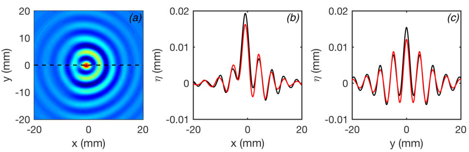 Figure 1
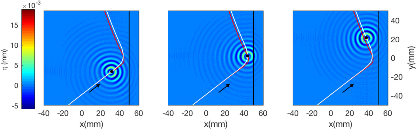 Figure 2
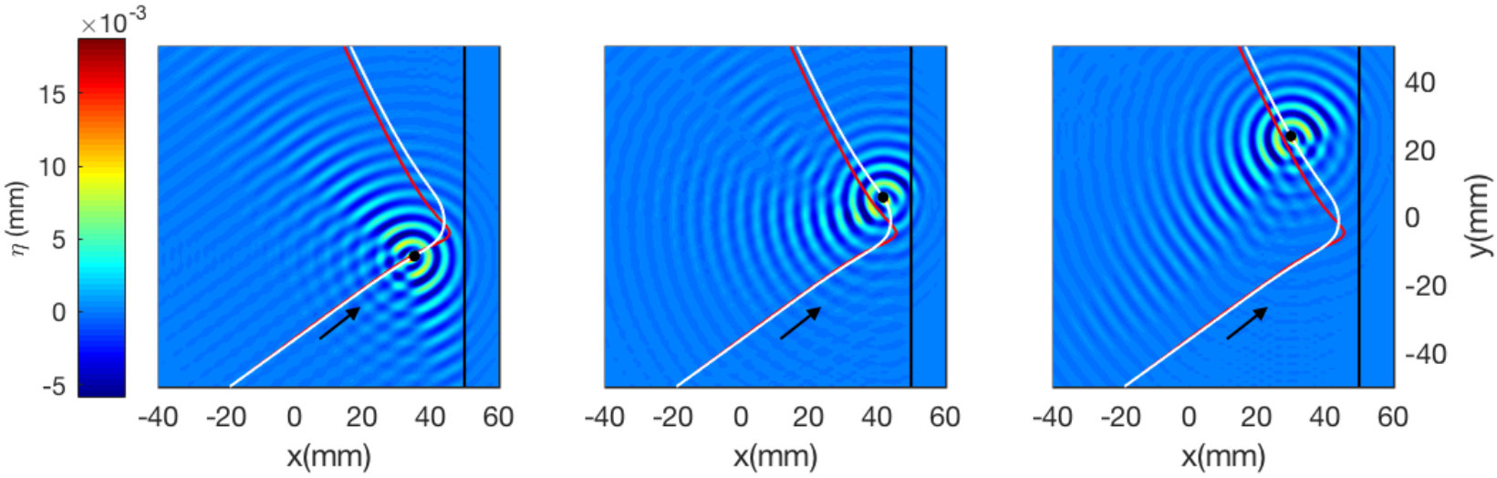 Figure 2
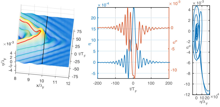 Figure 3
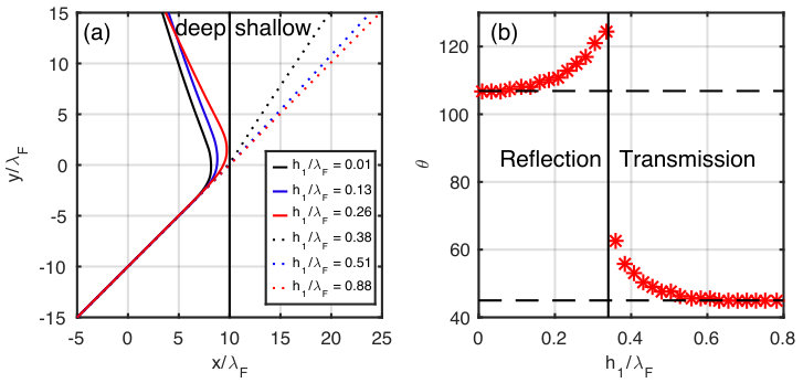 Figure 4
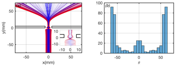 Figure 5
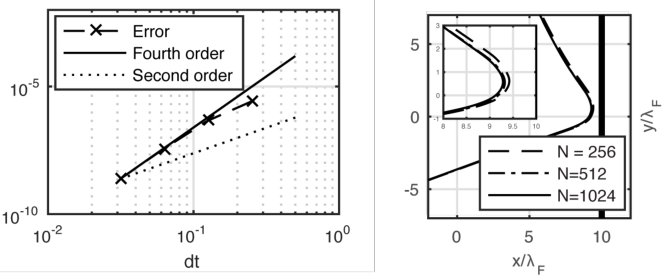 Figure 6
| Symbol | Meaning | Typical value |
|---|---|---|
| Dynamic viscosity | 20 cSt | |
| Effective viscosity | cSt | |
| Surface tension | 0.0206 N/m | |
| Density | 949 kg/ | |
| Driving frequency | 80 Hz | |
| Driving amplitude | 0 – 4.22 | |
| Faraday threshold for | 4.22 | |
| Depth in the deep region | 6.09 mm | |
| Depth in the shallow region | 0.42 mm | |
| Faraday wavenumber in the deep region | 1.265 | |
| Faraday wavenumber in the shallow region | 1.555 | |
| Coefficient of tangential restitution | 0.17 |
| Drop radius 0.39mm | Drop radius 0.335mm | ||||
|---|---|---|---|---|---|
| v(mm/s) | v(mm/s) | v(mm/s) | |||
| 11.1 | 0.345 | 11.45 | 0.3 | 6.6 | 0.275 |
Peer Reviews
No public reviews on file for this paper yet. If you reviewed it on a platform where reviews are public (OpenReview, ICLR, NeurIPS, ICML), you can paste yours below so the community can read it here.
Videos
No videos yet. Explain this paper in a talk, walkthrough, or lecture? Add one.
A model for Faraday pilot-waves over variable topography
Luiz M. Faria
Department of Mathematics, Massachusets Institute of Technology, Cambridge, MA 02139, USA
Abstract
Couder and Fort [8] discovered that droplets walking on a vibrating bath possess certain features previously thought to be exclusive to quantum systems. These millimetric droplets synchronize with their Faraday wavefield, creating a macroscopic pilot-wave system. In this paper we exploit the fact that the waves generated are nearly monochromatic and propose a hydrodynamic model capable of quantitatively capturing the interaction between bouncing drops and a variable topography. We show that our reduced model is able to reproduce some important experiments involving the drop-topography interaction, such as non-specular reflection and single-slit diffraction.
1 Introduction
The most mysterious manifestation of particle-wave duality certainly belongs to the quantum world. Our intuition, formed primarily by experiencing particles and waves at macroscopic scales, appears to be of little use when trying to rationalize the inherent duality of subatomic objects. At the heart of quantum mechanics lies this duality, where electrons are at times waves, diffracting, and at times particles, hitting a screen. Recently, a series of fluid dynamics experiments has provided an interesting example of particle-wave association at the macroscopic scale. The experiments consist of releasing a millimetric drop on the surface of a periodically oscillating bath. Given the right combination of parameters, the drop avoids coalescence by always maintaining an air layer between itself and the free-surface [33]. Such a drop can bounce indefinitely on the surface, generating a wave-field around its position. Furthermore, as the parameter controlling the amplitude of the periodic forcing is increased, the drops can be shown to go through an instability and start moving horizontally, giving rise to what are commonly called walkers [8]. Since the waves are generated by the drops, and the drops propelled by the waves, the system comprises a macroscopic analogy of the pilot-wave theory of quantum mechanics as first conceived by [11].
Several studies have further explored the analogies between bouncing drops and quantum mechanics. [7] demonstrated that walkers diffract through single- and double-slits in a manner reminiscent to electron/photon diffraction [2]. [13], showed that walkers can tunnel through submerged boundaries, analogous to quantum tunneling. [15] established that, when in a rotating frame, walkers settle into circular orbits of quantized radii, providing an analogy to Landau quantization (see also [27, 17]). [29] and [21] examined walker motion in a central force, and reported the emergence of a double quantization in energy and angular momentum. [18] studied walkers in a circular bath, and demonstrated the emergence of coherent statistical behavior similar to what is observed in quantum corrals [9].
Central to the understanding of this hydrodynamic pilot wave system is the concept of memory [7, 14]. Every time the drop bounces on the vibrating surface, it generates a wave which decays exponentially in time due to the viscous dissipation. Upon several impacts, the wavefield is thus the accumulation of all contributions from previous impacts. The ability of a drop to “remember” its past depends crucially on the decay rate of the waves. Near the Faraday threshold, the waves decay slowly, and the drop’s dynamics will depend not only on its current position, but also on the position of its previous impacts. This is, in essence, the source of the temporal non-locality displayed by bouncing drops, and represents a key idea in most theoretical models [30, 7, 14, 21, 25, 28].
Despite significant progress in the theoretical understanding of this hydrodynamic pilot-wave system, an important gap still exists: the interaction of walkers with variable topography. Such interactions give rise to apparently non-classical behaviour of the drops and arise in a number of key hydrodynamic quantum analog systems. Therefore an ability to model these interactions will be crucial to better understanding the analogy –and the limitations thereof– between the macroscopic pilot-wave system and its quantum counterpart. Most of the theoretical models developed in the past (see [6] for a review) focus on baths of effectively infinite depth. A few recent exceptions include [26], [16], [5], and [12]. In [26] conformal mapping is used to transform a variable topography to a flat one, a technique limited to two-dimensions. In [16] and [5] the variation in depth is treated as an effective boundary, and the wavefield is decomposed into eigenfunctions of the Laplacian with either a homogenous Neumann [16] or Dirichlet [5] boundary condition. [12] takes an approach similar to [16] in imposing a homogenous Neumann condition at the effective boundaries, but the equations are solved employing a Green’s function approach instead of an eigenfunction decomposition as in [16].
In this paper we propose a reduced model rich enough to capture the interaction between walkers and variable topography, yet simple enough to allow for efficient numerical simulation and physical transparency. Unlike the works cited in the previous paragraph, the variable depth is treated not as an effective boundary, but as a place where the wave speed changes, providing a mechanism for wave reflection. The model exploits the fact that, because the entire system is driven near resonance, the wavefield is nearly monochromatic and therefore only certain wavenumbers need to be modeled correctly. We show that –with a reasonable quantitative agreement– our model reproduces some important laboratory experiments such as non-specular reflection [13, 32] and the observed pattern of diffraction past a slit reported in [19].
2 Model
In this section we present the theoretical model. In §2.1, we develop a simplified description of the surface waves, and in §2.2 we incorporate the effect of drops bouncing on the surface.
2.1 Surface waves model
We are interested in the surface waves of a bath undergoing a vertical sinusoidal oscillation. In the bath’s frame of reference, the problem is equivalent to considering a time dependent gravity: , where is the gravitational acceleration, denotes the angular frequency of oscillation, and the amplitude. For a fixed , there exists a critical amplitude of oscillation, , above which the surface becomes unstable. In the nearly inviscid limit of interest to this paper, the instability is always subharmonic, with frequency [4, 20]. The bouncing drop experiments described in the introduction are typically carried out near (and below) the stability boundary, so that the flat surface of the bath is stable, but subharmonic modes excited within it decay very slowly. Furthermore, the drops are small enough that the waves they generate may be treated as linear.
Instead of beginning with the linearized Navier-Stokes equations, we take as a starting point the quasi-potential theory developed in [23], which when extended to a bath of finite depth is given by
[TABLE]
Here , denote the free-surface displacement and velocity potential. The parameter is an effective kinematic viscosity, chosen to capture the correct stability threshold , and denote surface tension and density. Finally, is a vector normal to the bottom profile, the depth of the undisturbed surface, and the horizontal Laplacian (i.e. ).
We consider a bath having a deep and a shallow region, separated by a discontinuous jump, so is given by:
[TABLE]
where . The key feature that we aim to exploit is that the sinusoidal oscillations of the bath favor the resonating temporal frequencies, causing the waves to be nearly monochromatic. Thus we need not model all waves correctly, but only those for which the frequency is approximately ; other waves are less important owing to their faster temporal decay.
The main difficulty in solving (1)–(4) is that in equation (4) couples the surface evolution to Laplace’s equation in the three-dimensional domain, making the problem computationally expensive. When , it can be shown that (see e.g. [34])
[TABLE]
where denotes the two-dimensional Fourier transform in and , and is the wavenumber vector. This allows for the surface evolution to be represented, in Fourier space, using only data on the surface, reducing a 3 dimensional problem to 2 dimensions. When is not constant, however, no simple explicit representation of in terms of exists. Our goal is to approximate in equation (4) using data on the surface only, and to do so in a way that correctly models waves with frequency .
Motivated by shallow water theory, we seek an approximation of the form
[TABLE]
and choose to exactly match the dispersion relation of Faraday waves in both the shallow and deep regions. Given and , we must thus determine the most unstable wavenumber in each region, denoted by . Following Appendix A of [23], the Faraday wavenumber in each region of constant depth is computed by finding the which minimizes in the following expression:
[TABLE]
where is the ideal/inviscid dispersion relation, is the dissipation rate, and . Notice that this reduces to the well-known result of [4] when , and in that limit simply satisfy
[TABLE]
In order for (7) to exactly match the dispersion relation of Faraday waves in the regions of constant depth, we must choose
[TABLE]
This leads to the following wave model:
[TABLE]
where is given by equation (10).
It is worth noting that in the long wave limit (i.e. ), we have that , and formally the linear shallow water theory is recovered. Our approximation, however, does not rely on , which is not typically true for the bouncing drop experiments, but on the assumption that the wave-field is nearly monochromatic, with all the energy in modes of temporal frequency near . For drops bouncing periodically over a vibrating bath, parametric resonance ensures that such an approximation is justifiable, as later shown in the quantitative comparison performed in Figure 1. In the next section we modify the wave model given by equations (11)–(12) in order to account for a drop bouncing on its surface.
2.2 Drop dynamics and wave/drop coupling
The wave-drop coupling is identical to that of [23] and [25], where the drop is treated as an excess pressure on the dynamic surface condition. This leads to the following system:
[TABLE]
The new term represents the effect of the drop, and denotes the drop’s horizontal position, which evolves according to
[TABLE]
The parameters , and denote the drop mass, drop radius, air viscosity, and coefficient of tangential restitution, respectively [25]. The function represents the reaction force exerted on the drop by the fluid.
Calculating requires solving for the vertical dynamics of the particle, which as shown in [24] can be well approximated by a logarithmic spring during contact. Although it is possible to couple the wave model here presented to the log-spring model of [24], for the sake of simplicity we assume that the drop bounces periodically, with period . It can then be shown (see [25]) that . Assuming that the contact time is small enough (relative to the bouncing period) that may be treated as an impulse force, and taking the impacts to happen at , we obtain , where is the Dirac delta function. This eliminates the need to solve for the vertical motion of the drop; however, by considering the impact to be instantaneous, the model ignores the evolution of the waves during contact, which may be important for certain types of interaction given that the contact time can be as large as one-fourth of the period. Finally the excess pressure may be modeled as , where describes the spatial distribution of the excess pressure ( and has units of ).
It is now convenient to nondimensionalize the equations using a representative length scale, , and time scale . Using tildes for dimensionless variables, we obtain
[TABLE]
where , , , , and denotes the impact phase. Similarly equation (15) becomes
[TABLE]
where and .
The last simplification comes from considering a point impact: . Equations (16)–(18) represent the final form of our model, and the rest of this paper is devoted to their study. Henceforth, we drop the tilde notation, but all variables are assumed dimensionless unless otherwise stated.
3 Numerical results
We solve equations (16)–(18) numerically using a pseudo-spectral method in space, and fourth order Runge-Kutta scheme for the time integration. Because of the temporal delta functions, we resolve the drop/surface interaction analytically during impact. That is, at we modify and by integrating our equations from immediately before until immediately after the impact (see Appendix A for details on the numerical algorithm). Doing so allows for high order accuracy in time without having to resolve the details of the drop/bath interaction. Convergence tests performed indicate that indeed fourth-order accuracy is achieved, and that the results do not depend substantially on the number of spectral modes employed (Appendix B).
For the numerical simulations that follow, we choose parameters appropriate for a fluid of cSt shaking at a frequency of Hz. Surface tension is N/m, and the density is kg/. In the deep region the depth is mm. When obstacles are present the depth above them is (unless otherwise indicated) mm, chosen to correspond roughly to the experiments of [32] and [19]. Computing using the method outlined in §2.1 yields mm and ; is then computed using (10). In order to compare our simulations to available experiments, two different drop sizes are considered: in subsections § 3.1–3.2 the drops have a radius of mm, while in § 3.3 they have a radius of mm. The coefficient of tangential restitution is taken to be , as suggested in [25] for a bath of cSt shaking at Hz. Finally, the effective viscosity is , which yields as the Faraday threshold for the fluid considered. The computations were performed on a domain of (dimensionless) size using points, which was sufficient to guarantee resolution-independent results (see Appendix B). All parameters used are summarized in Table 1.
We present below three examples that illustrate the capabilities of the model. First, in § 3.1, we briefly study the dynamics of a drop in a bath of constant depth. We then explore in § 3.2 the interaction of walkers with a planar submerged step, demonstrating that our model captures many of the important features of walker reflection. Finally, we present in §3.3 results of diffraction past a single slit.
3.1 Constant depth
We consider first walkers in a uniform bath as a benchmark for the model. As expected, in the absence of barriers the drops move at a constant speed that is independent of the initial conditions. For any fixed set of physical parameters, the final free-space velocity will depend only on the impact phase . Because we have chosen not to consider the details of the vertical dynamics, is extraneous to the model and may therefore be treated as a free parameter. As in previous strobed models that average out the vertical dynamics (e.g. [28], [21]), is chosen so that the theoretical walking speed approximately agrees with the experimentally reported value. A summary of the average experimental walking speed, as well as the inferred impact phase used for all configurations reported in this paper can be found in Table 2.
The first comparison we perform is between our model and the equations they are intended to approximate, specifically (1)–(4). We show in Figure 1 the wave-field generated by a walker using our nearly monochromatic approximation, and compare it to the wave-field obtained when using the quasi-potential theory of [23]. Although the match is not perfect, the overall wave features appear to be correctly captured. This indicates that, at least in places of constant depth, where it is easy to solve for exactly using (6), our monochromatic approximation performs reasonably well. In the next sections, when considering a variable bottom topography, it becomes very difficult to solve (1)–(4); therefore, in §3.2 we instead compare our model to experimental observations of [32] and [19].
3.2 Reflection from planar boundary
We consider now one of the simplest types of walker-boundary interactions: reflection from a planar submerged obstacles, and compare two of our trajectories to the experimental data of [32]. The simulation consists of sending a walker towards a shallower region at a given incident angle and then recording both the trajectory and the wave-field for several hundred impacts. The walker-boundary interaction can be divided into three distinct stages, depicted in Figure 2 for two different values of . First, at sufficient distance from the shallow region (mm in Figure 2), the walker does not feel the presence of the step, and therefore moves in a straight line. Then, as it approaches the barrier, its reflected waves start to affect the dynamics, eventually causing the walker to turn around. The drop continues to interact with the submerged step through its wave-field as it moves away from it: the trajectory appears to curve towards the step, becoming asymptotic to a rectilinear motion.
At high memory (Figure 2(b)), we also see the formation of interference fringes caused by the reflected waves. Finally, we observe that although the model approximately captures the correct reflection angle (experimental and numerical lines are nearly parallel in Figure 2), the details of the trajectory near the wall are slightly different from the experiments, where the experimental trajectories turn more sharply. Interestingly, the reflection is non-specular (i.e. incident and reflected angles are not equal), and there is a small preferred range of reflected angles. A detailed study of the walker’s non-specular reflection, as well as a more through comparison between the theory here developed and experiments, is reported in [32]. We also see in Figure 2 that, as expected, the waves have a much smaller amplitude in the shallow region () than in the deep region (). However, neither nor appears to be zero at the deep-shallow interface. This inference, consistent with the schlieren imaging of [13] and [10], suggests that imposing an effective Dirichlet or Neumann boundary condition on the wavefield at places where the depth changes is likely to be inadequate.
In order to study in more detail what happens to at the deep-shallow interface, we consider in Figure 3 a walker impinging perpendicularly upon the step. The drop’s trajectory remains orthogonal to the step at all times, allowing for an easier study of the waves by focusing on the x cross-section of the wavefield. We show in Figure 3a the x cross-section of the wavefield as a function of time (i.e. ), where has been chosen as the time where the drop turns away from the shallow region. We see that within about wavelengths into the shallow region the wave amplitude has already decayed to nearly zero. The behavior of above the step, indicated by the black line in the figure, suggests that neither nor holds at the deep-shallow interface. This is better seen in Figure 3b, where we plot and at (i.e. above the step) as a function of time. We see that, as the drop approaches the wall, the wave height above the step (blue curve in Figure 3b) oscillates in time, indicating the presence of a transmitted wave.
The relationship between and at the deep-shallow interface, plotted in Figure 3c, appears to be rather complex. If the variable depth in the fluid were to be modeled by means of an effective boundary condition of the Robin type, i.e. , then Figure 3c should show (at least approximately) a straight line; for the depth ratio considered in Figure 3, this is not the case. Thus, in the context of our model, an effective boundary condition of the Robin type cannot be used in lieu of the spatially varying coefficient in the PDE without sacrificing quantitative agrement, and a more complex boundary condition must be sought. Of course, it may very well be that in certain limits (e.g. as ) the relation between and becomes simple, and an effective boundary of the Robin type becomes appropriate.
We also use the model to investigate the effect of the height above the step on the trajectory. In Figure 4 we consider a walker coming from a deep region (mm) and impinging upon a step at an angle of . We vary the depth above the step between mm and mm by small increments, and then calculate the final angle after the walker has interacted with the step. We see that the final angle appears to asymptote to a constant for either very shallow or very deep steps. The drops is unable to feel the bottom (i.e. the trajectories do not significantly deviate from a straight line) for depths larger than . For depths less than , we also see that the reflection angle depends only weakly on the depth. This observation, consistent with experiments (G. Pucci, private communication), suggests that as long as the depth above the obstacles is small enough, the drop’s interaction with boundaries will be largely independent of the depth in the shallow region .
3.3 Diffraction by a slit
We now briefly consider the case of a walker launched towards a slit. If the drop behaved like a classical macroscopic particles, we would expect its trajectory to remain unaffected by the passage through a slit. In [7], it was shown that this is not the case: passage through a slit deflects the drop owing to the interaction of its wavefield and the barrier. It was found that walkers behaved (on average) much like a plane wave diffracted through a slit. Subsequent experiments conducted by [19], [1], and [3], were unable to reproduce the precise diffraction pattern observed in [7]. Nevertheless, walker deflection was apparent in all of them. [19] found that, in the absence of external air currents, the single-slit trajectories were dominated by two preferred angles similar to those emerging in the reflection experiments. We proceed by showing that our numerical simulations are consistent with the findings reported in [19].
The bath topography consists of a deep region of depth mm, and shallow region, in the shape of a slit, of depth mm (see figure 5). The width and breadth of the slit are respectively mm and mm wide. Letting be the distance of the initial position of the drop from the center of the slit, we took a uniform sample of trajectories with impact parameters ranging from [math]mm to mm by increments of mm (300 cases in total). Trajectories with mm reflected from the barrier, and were thus discarded. All simulations started at mm, which ensures that a steady walking state is achieved prior to interaction with the slit. We set , and considered a drop of radius mm, corresponding to the parameters examined by [19].
In figure 5a we show a few sample trajectories of our numerical simulations. The slit appears to focus trajectories inside it: its width plays an important role in the dynamics. The observed pattern does not appear to be of the classical wave diffraction type; in fact, most trajectories settle to a small range of angles after passing through the slit, which is reminiscent of the planar wall reflection and consistent with the findings reported in [19]. Plotting a histogram of the final angle of each trajectory (Figure 5b), indicates a strong preference for , which is similar to the preferred angle observed in [19]. The number of bins in figure 5b was chosen to be approximately , where is the number of trajectories considered. The main qualitative feature of the histogram, i.e. its lateral peaks, remains unaffected by variations in bin size. A thorough comparison between our model and recent single and double-slit experiments will be reported in [31].
4 Conclusions
We have presented a model capable of capturing many interesting features of walker-topography interactions. The model treats depth changes in the fluid not as boundaries, but as regions where the wave speed changes, effectively creating a mechanism for partial wave reflection. Although our equations are reminiscent of a long wave approximation, we demonstrate that the model remains useful outside the shallow-water limit provided the system is driven near resonance, and the drop is synchronized with its Faraday wavefield.
The assumption that the drop’s vertical motion is periodic, and in resonance with the Faraday waves, might limit the applicability of the model to resonant walkers. In fact, even drops in the resonant modes may alter their vertical motion, or even violate the periodic assumption, when interacting with other drops or obstacles. Surprisingly, a reasonable agreement is still observed in practice (e.g. Figure 2), even though we neglect the vertical dynamics. Inclusion of vertical dynamics into our model is a possible direction of future research.
Our treatment of the variable topography captures the important properties of the reflected waves without a need to explicitly impose a boundary condition. Although it would be interesting to develop a systematic understanding of the reflected Faraday wave, the viscous dissipation and time-dependent gravity are likely to make a rigorous analysis of the reflection and transmission laws at a depth discontinuity extremely challenging, even in the context of our simplified model. Direct numerical simulations of (1)–(4) are also a possible future direction to better understand the Faraday pilot-waves over variable topography, although the computational cost of such a task is likely to be daunting.
The choice of given by equation (10) was made so as to correctly capture the phase velocity of the Faraday waves. The approximation of given by equation (7), however, is too simple to allow for the model to also capture the group velocity of the Faraday waves correctly. Interestingly, as shown in the comparison presented in Figure 1, the group velocity of the Faraday waves does not appear to fundamentally affect the structure of the drop/pilot-wave ensemble. Employing more sophisticated approximations to that also capture the group velocity of the Faraday waves is likely to improve the quantitative agreement with the quasi-potential theory of [23], and is a direction currently being pursued.
Finally, we note that all nonlinearities in this hydrodynamic system arise from the particle-wave coupling, which gives rise to complex behavior that is neither particle-like nor wave-like. The precise nature of the coupling is thus extremely import, and cannot be overlooked in any pilot-wave theory. Although the recent experiments of [1] and [19] do not yield the specific diffraction pattern reported in [7], it is clear that particle-wave duality is at the of heart of the bouncing drops’ quantum-like features. For example, trajectories deflecting past a slit give clear evidence of the dual nature of bouncing drops. The relevance of this classical wave-partical duality to quantum mechanics remains, of course, an open question. Nevertheless, bouncing drops do provide an enticing physical picture, even if only at the level of analogy, of what may be happening at scales that we cannot yet probe.
Acknowledgements: I am grateful to John Bush, Aslan Kasimov, Andre Nachbin, and Ruben Rosales for fruitful discussions. I would also like to thank Giuseppe Pucci and Pedro Saenz for making their experimental data available.
Appendix A Details of numerical algorithm
In this section we explain how the governing equations are solved numerically. The (dimensionless) particle-wave system considered is governed by (see section §2.2):
[TABLE]
where . Since the impacts are instantaneous (i.e. is a sum of delta functions), it is convenient to divide the time evolution in two parts: impact and free-flight. The algorithm consists of two main routines: one which evolves the particles and the waves during free-flight, and another which resolves the details of the impact.
During free-flight the wave evolution is solved using a (Fourier) pseudo-spectral method in space. Taking the Fourier transform of (19)–(20), and assuming so that , yields
[TABLE]
The time evolution of the waves is carried in Fourier space by a standard fourth order Runge-Kutta method (e.g. [22]). The topography enters through the term , which is numerically computed pseudo-spectrally in the following way:
[TABLE]
For the topography considered in the paper, is a discontinuous function, and the Fourier transform in (24) will be subject to the well known Gibbs phenomenon. Although in principle this could generate numerical stability problems and/or degrade the accuracy of the algorithm, we observed that in practice the damping provided by the viscous terms in (19)–(20) was enough to smooth the solution sufficiently so that no numerical instabilities were observed (see also Appendix B for convergence tests). Similarly, during free-flight the particle evolves according to , which is solved analytically.
During impact, we exploit the temporal delta function present in the model to resolve the interaction analytically. That is, at impact times we modify and by integrating our equations from immediately before until immediately after an impact. For the surface potential , integration of (22) across an impact can be easily shown to yield:
[TABLE]
where the plus and minus superscripts denote values immediately after and immediately before the impact, respectively. Integration of (21) requires a bit more care since the friction term contains a delta function, which multiplies , a discontinuous term. For simplicity we consider the case of a single impact at . Immediately before the impact both and are known, and continuity of both across the impact implies and . For convenience, we define . Resolving (21) across an impact is then equivalent to solving
[TABLE]
We proceed formally by multiplying (26) by the integrating factor , yielding:
[TABLE]
and so
[TABLE]
Solving for gives:
[TABLE]
which is used in the algorithm to update the drop’s velocity at each impact111A more rigorous way to proceed is to consider an mollification of the Dirac delta, solve (26) with replaced by the and then take the limit at the end. The final result of this procedure is the same as that obtained from our formal calculation..
Appendix B Convergence tests
In this section we investigate the effect of the numerical resolution on the results obtained. First we verify that the walking speed in freespace is not a function of the resolution, and that as the time steps are decreased the algorithm converges with fourth order accuracy. This is shown in Figure 6a, where we plot the error in the free-walking speed as a function of for a fixed spatial resolution of 512x512 modes. Each simulation was ran until the walker’s speed saturated to a constant, and the maximum error (relative to a very fine simulation) over the last 50 impacts was computed. Clearly, despite our treating the drop as a delta function in space and time, fourth order convergence is still recovered.
In Figure 6 we verify that the resolution of 512x512 spectral modes in a domain of size 64x64, which was used in the simulations presented in §3, is sufficient to obtain a reliable result even in the presence of a piecewise constant topography. More precisely, we plot the trajectory of a walker undergoing reflection using 256, 512, and 1024 spectral modes in each direction. As can be seen in Figure 6b, the difference between using 512 and 1024 modes was sufficiently small that 512 was considered an acceptable resolution (in fact the final reflection angles predicted using 512 or 1024 modes vary by less than ).
The reference list from the paper itself. Each links out to its DOI / PubMed record.
- 1[1] Anders Andersen, Jacob Madsen, Christian Reichelt, Sonja Rosenlund Ahl, Benny Lautrup, Clive Ellegaard, Mogens T Levinsen, and Tomas Bohr. Double-slit experiment with single wave-driven particles and its relation to quantum mechanics. Physical Review E , 92(1):013006, 2015.
- 2[2] Roger Bach, Damian Pope, Sy-Hwang Liou, and Herman Batelaan. Controlled double-slit electron diffraction. New Journal of Physics , 15(3):033018, 2013.
- 3[3] Herman Batelaan, Eric Jones, Wayne Cheng-Wei Huang, and Roger Bach. Momentum exchange in the electron double-slit experiment. In Journal of Physics: Conference Series , volume 701, page 012007. IOP Publishing, 2016.
- 4[4] T Brooke Benjamin and F Ursell. The stability of the plane free surface of a liquid in vertical periodic motion. Proceedings of the Royal Society of London. Series A, Mathematical and Physical Sciences , pages 505–515, 1954.
- 5[5] François Blanchette. Modeling the vertical motion of drops bouncing on a bounded fluid reservoir. Physics of Fluids , 28(3):032104, 2016.
- 6[6] John WM Bush. Pilot-wave hydrodynamics. Annual Review of Fluid Mechanics , 47:269–292, 2015.
- 7[7] Yves Couder and Emmanuel Fort. Single-particle diffraction and interference at a macroscopic scale. Physical review letters , 97(15):154101, 2006.
- 8[8] Yves Couder, Suzie Protiere, Emmanuel Fort, and Arezki Boudaoud. Dynamical phenomena: Walking and orbiting droplets. Nature , 437(7056):208–208, 2005.