The JCMT Gould Belt Survey: A First Look at IC 5146
D. Johnstone, S. Ciccone, H. Kirk, S. Mairs, J. Buckle, D.S. Berry, H., Broekhoven-Fiene, M.J. Currie, J. Hatchell, T. Jenness, J.C. Mottram, K., Pattle, S. Tisi J. Di Francesco, M.R. Hogerheijde, D. Ward-Thompson, P., Bastien, D. Bresnahan, H. Butner, M. Chen, A. Chrysostomou

TL;DR
This study presents submillimetre observations of IC 5146, identifying dense clumps, analyzing their stability, and examining the relationship between protostars and these clumps to understand star formation conditions.
Contribution
It provides the first detailed submillimetre survey of IC 5146, characterizing clump properties, stability, and protostar correlations within different star-forming regions.
Findings
Most clumps are thermally Jeans stable.
Younger protostars are strongly associated with submillimetre peaks.
The Cocoon Nebula has a higher fraction of dense, unstable clumps with protostars.
Abstract
We present 450 and 850 micron submillimetre continuum observations of the IC5146 star-forming region taken as part of the JCMT Gould Belt Survey. We investigate the location of bright submillimetre (clumped) emission with the larger-scale molecular cloud through comparison with extinction maps, and find that these denser structures correlate with higher cloud column density. Ninety-six individual submillimetre clumps are identified using FellWalker and their physical properties are examined. These clumps are found to be relatively massive, ranging from 0.5to 116 MSun with a mean mass of 8 MSun and a median mass of 3.7 MSun. A stability analysis for the clumps suggest that the majority are (thermally) Jeans stable, with M/M_J < 1. We further compare the locations of known protostars with the observed submillimetre emission, finding that younger protostars, i.e., Class 0 and I sources,…
Click any figure to enlarge with its caption.
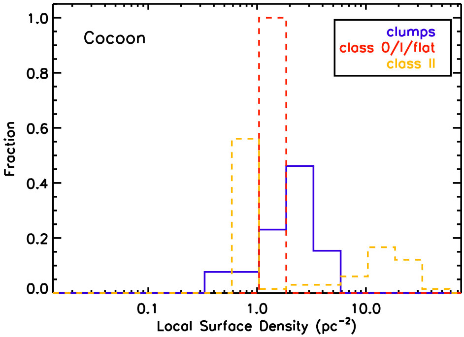 Figure 10
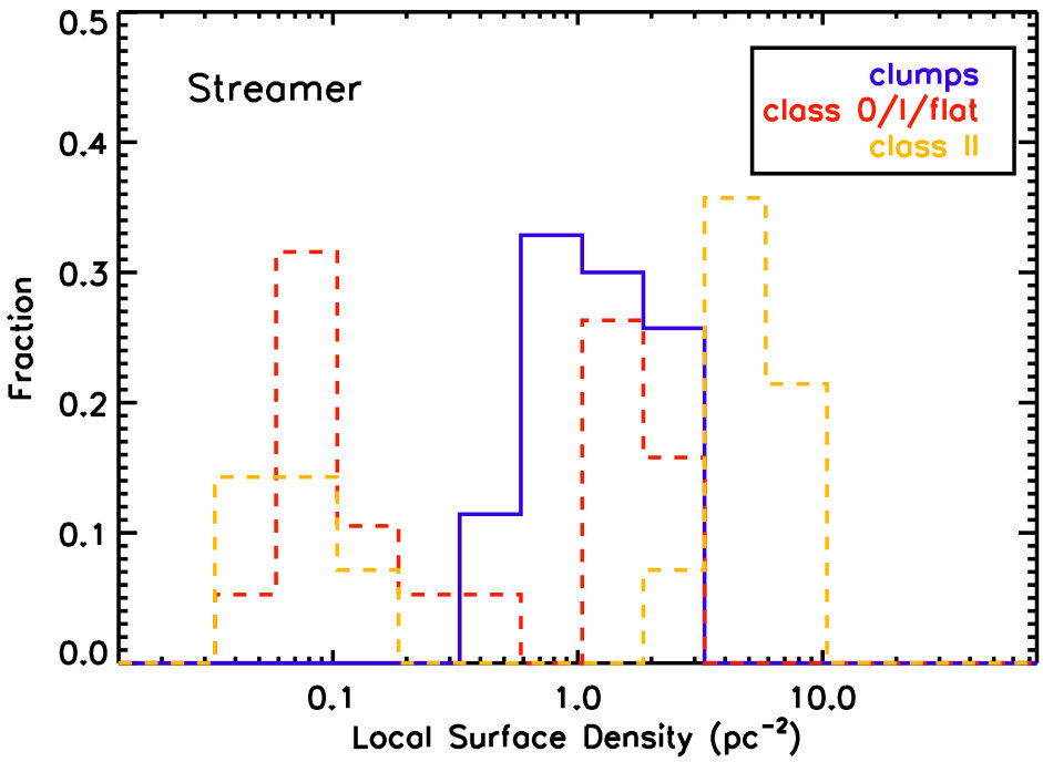 Figure 10
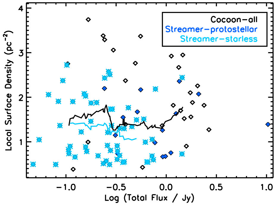 Figure 11
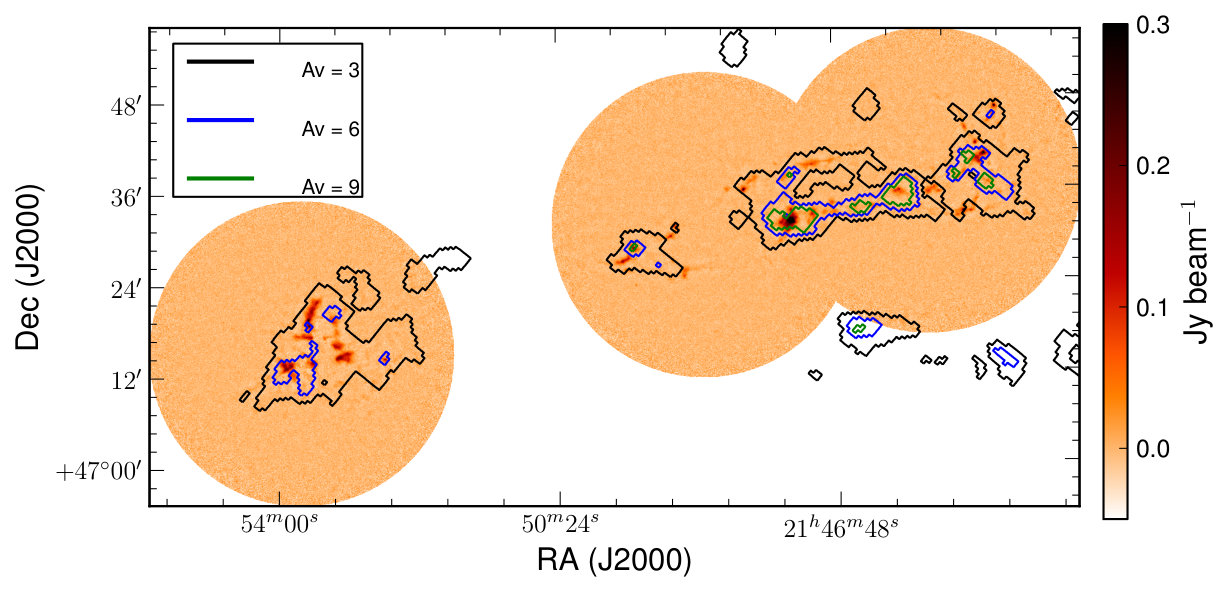 Figure 1
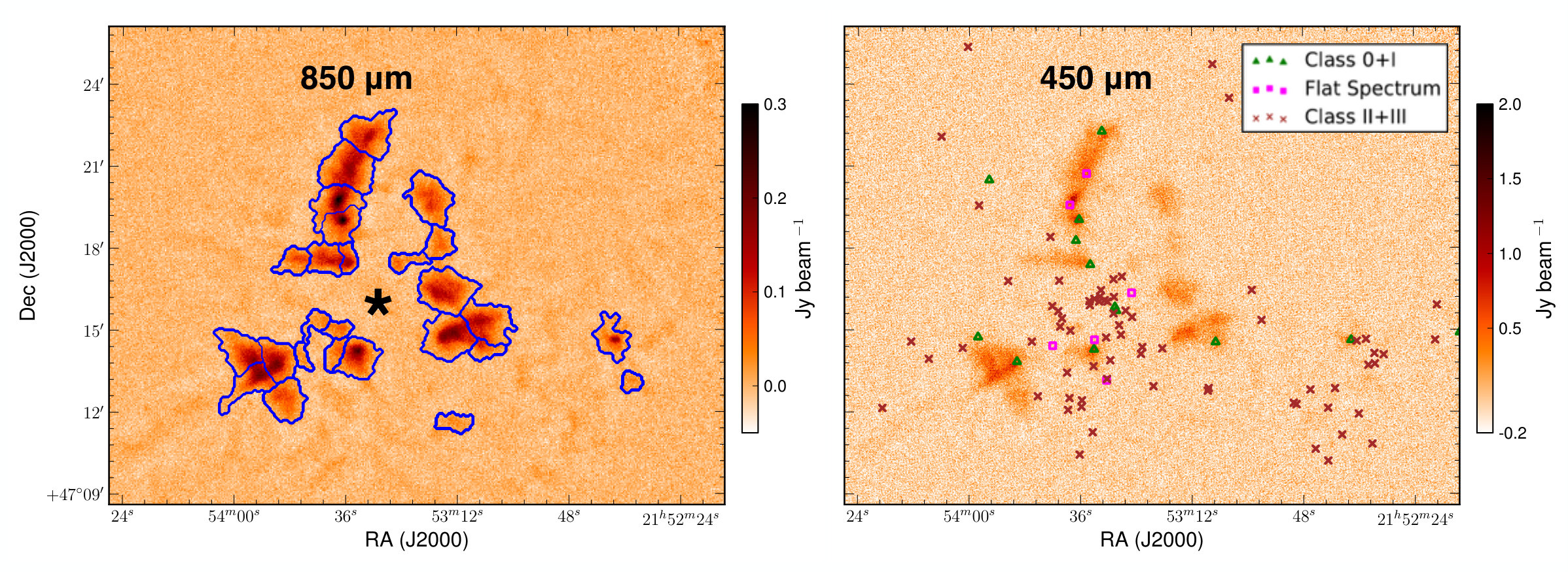 Figure 2
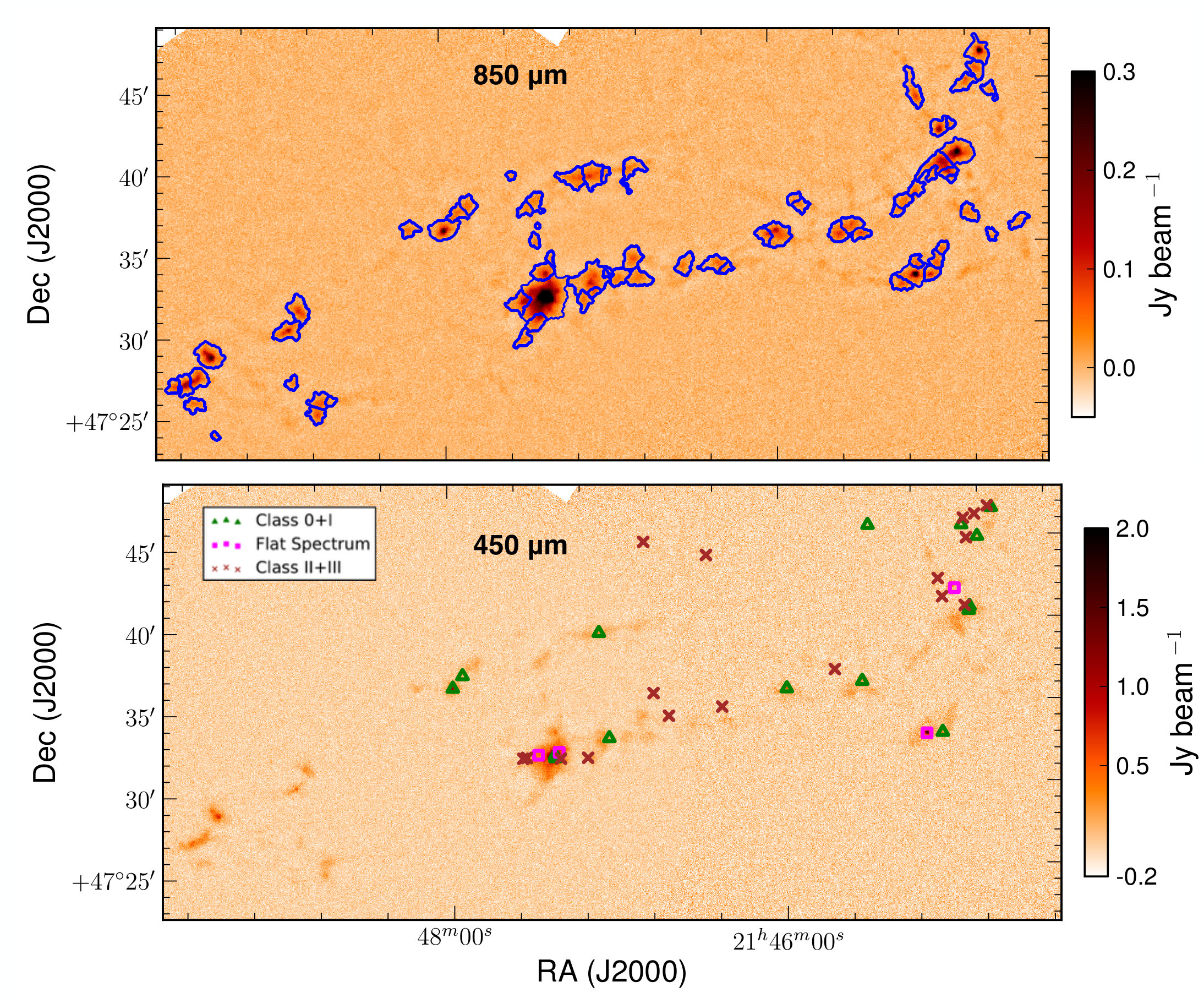 Figure 3
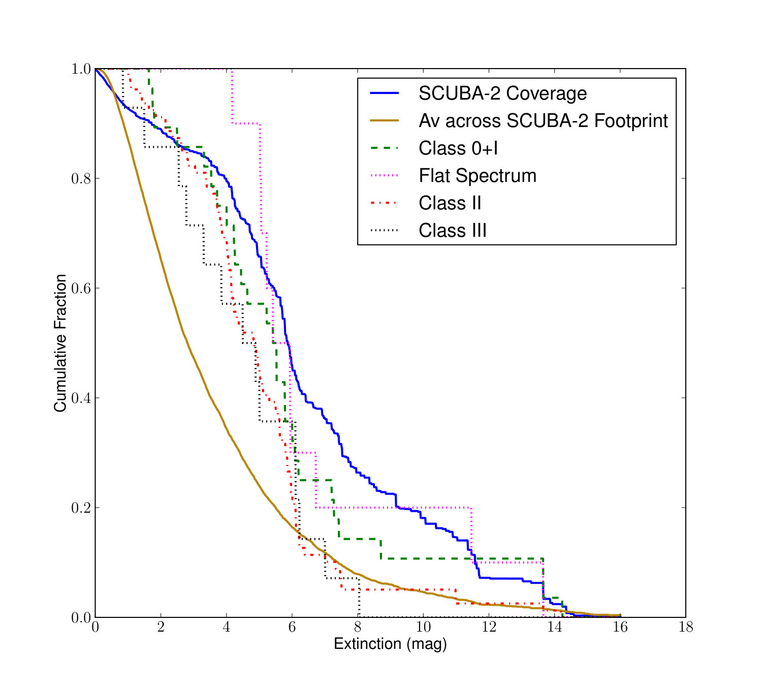 Figure 4
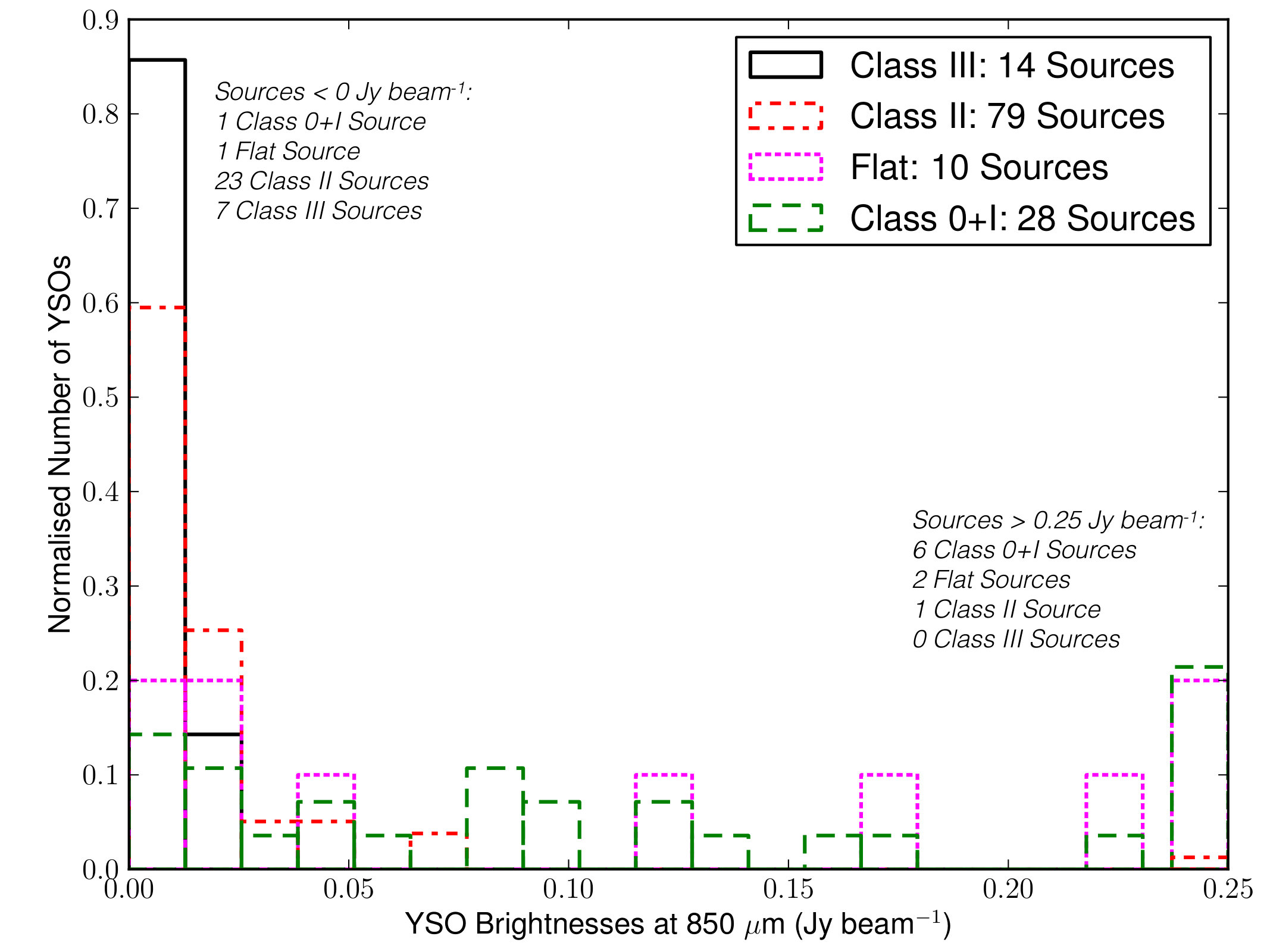 Figure 5
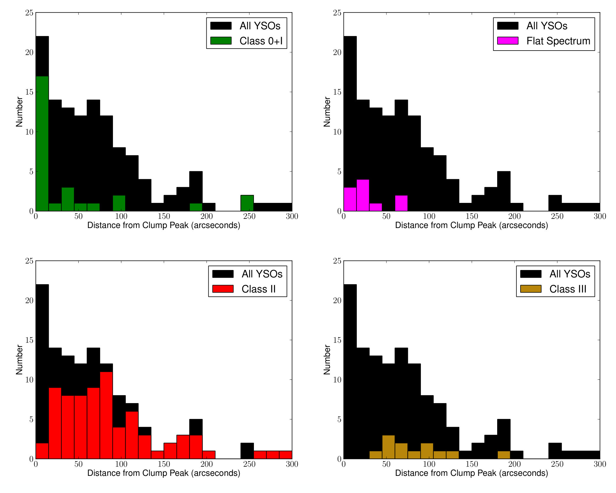 Figure 6
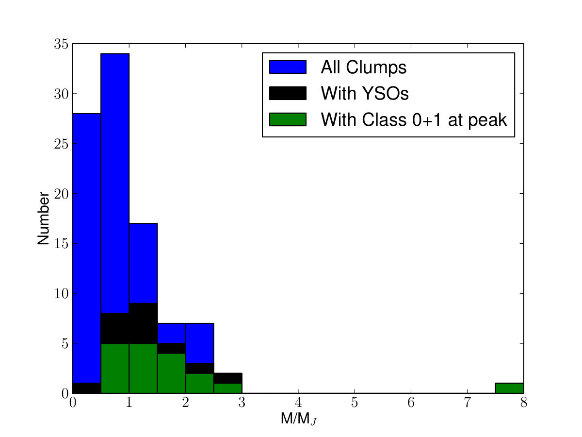 Figure 7
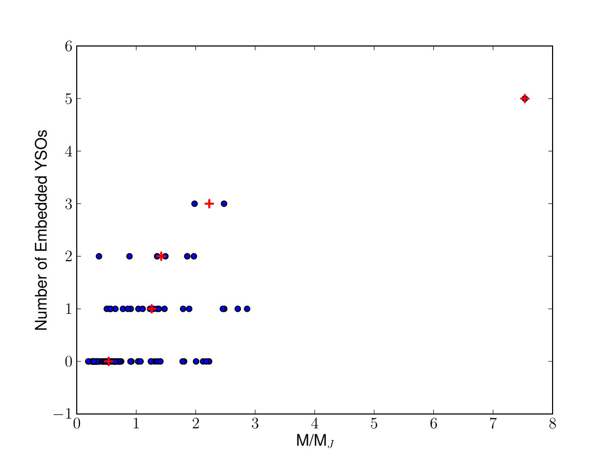 Figure 8
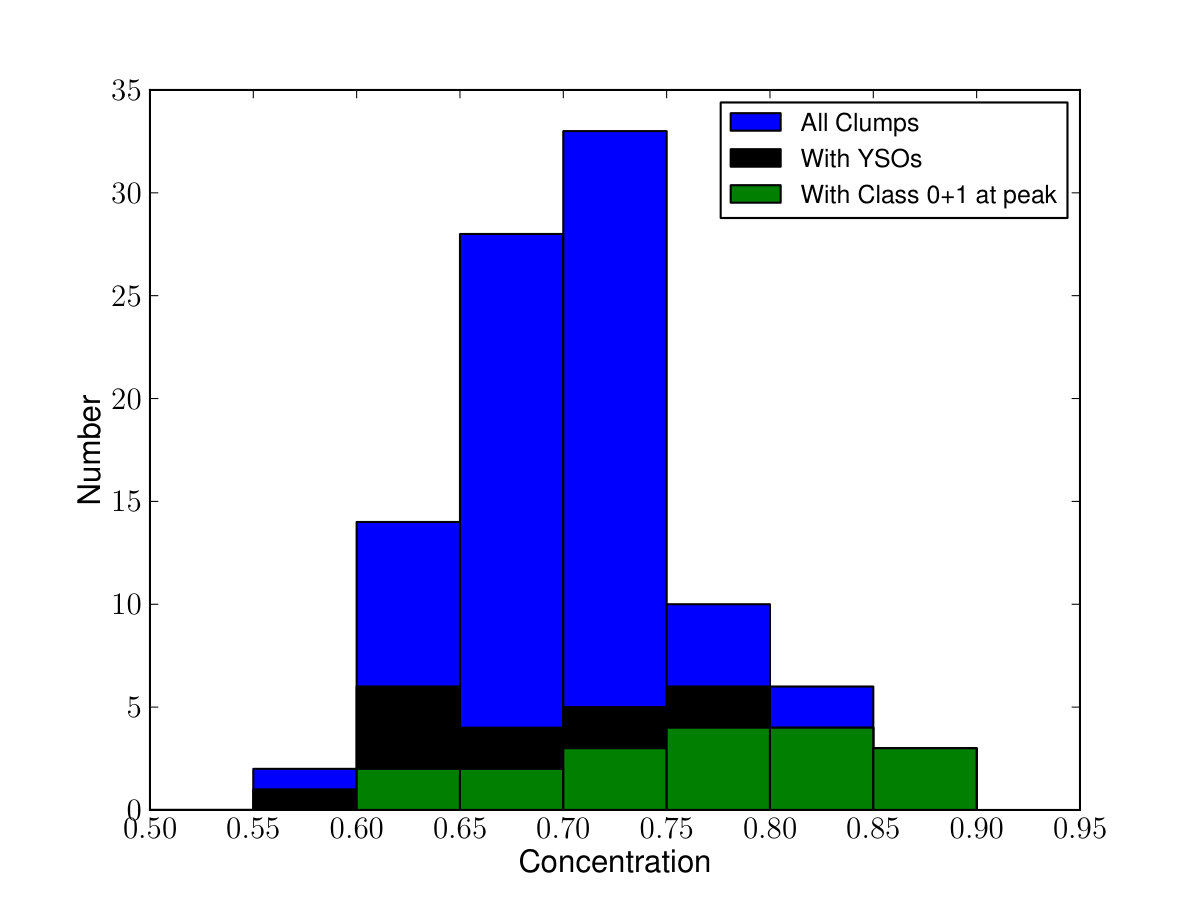 Figure 9
| Region | NameaaObservation designation chosen by GBS team, denoted as Target Name in the CADC database at http://www3.cadc-ccda.hia-iha.nrc-cnrc.gc.ca/en/jcmt/. The Proposal ID for all these observations is MJLSG36. | R.A.bbCentral position of each observation. | Dec.bbCentral position of each observation. | ccPixel-to-pixel (rms) noise within each region after mosaicking together all observations. | ccPixel-to-pixel (rms) noise within each region after mosaicking together all observations. | ddEffective noise per beam (i.e., point source sensitivity) within each region after mosaicking together all observations. | ddEffective noise per beam (i.e., point source sensitivity) within each region after mosaicking together all observations. |
|---|---|---|---|---|---|---|---|
| (J2000.0) | (J2000.0) | (mJy arcsec-2) | (mJy bm-1) | ||||
| Coccon Nebula | IC5146-H2 | 21:53:45 | 47:15:22 | 0.050 | 1.4 | 3.7 | 67 |
| Northern Streamer | IC5146-E | 21:48:31 | 47:31:48 | 0.045 | 1.1 | 3.3 | 53 |
| Northern Streamer | IC5146-W | 21:45:36 | 47:36:59 | 0.049 | 1.4 | 3.6 | 67 |
| Extinction | Cloud Area | Mext | Ms2 | Ms2/Mext | C0+I+F | CII | CIII | ||
|---|---|---|---|---|---|---|---|---|---|
| (mag) | (%) | (M⊙) | (%) | (M⊙) | (%) | (%) | (%) | (%) | (%) |
| S2 Coverage: 0 | 100 | 16051 | 100 | 670.3 | 100 | 4 | 100 | 100 | 100 |
| 2 | 30 | 10472 | 65 | 596.5 | 89 | 6 | 92 | 91 | 86 |
| 5 | 6 | 3844 | 24 | 440.7 | 66 | 11 | 66 | 46 | 43 |
| 10 | 1 | 742 | 5 | 121.4 | 18 | 16 | 13 | 5 | 0 |
| Cocoon Neb.: 0 | 100 | 5125 | 100 | 285.4 | 100 | 6 | 100 | 100 | 100 |
| 2 | 32 | 3479 | 68 | 88.7 | 31 | 3 | 100 | 91 | 89 |
| 5 | 5 | 976 | 19 | 29.4 | 10 | 3 | 79 | 46 | 44 |
| 10 | 0 | 0 | 0 | 0.0 | 0 | – | 0 | 0 | 0 |
| N. Streamer: 0 | 100 | 10926 | 100 | 384.9 | 100 | 4 | 100 | 100 | 100 |
| 2 | 28 | 6993 | 64 | 335.5 | 87 | 5 | 84 | 93 | 80 |
| 5 | 6 | 2868 | 26 | 240.0 | 62 | 8 | 53 | 43 | 40 |
| 10 | 1 | 742 | 7 | 121.4 | 32 | 16 | 26 | 29 | 0 |
| Name | Descriptor | Value |
|---|---|---|
| AllowEdge | exclude clumps touching the noisier map edge | 0.00 |
| CleanIter | smooth clump edges | 15.0 |
| RMS | as measured in the map | 0.05 |
| FlatSlope | increase the gradient required for associating pixels with a peak | 2.0*RMS |
| MinDip | reduce the difference between peaks required to have multiple objects | 1.5*RMS |
| MaxJump | reduce the search radius to combine peaks into a single object | 2.0 |
| MinPix | minimum number of pixels per clump | 10.0 |
| Noise | allow fainter pixels to be associated with a peak | 0.35*RMS |
| ClumpaaClump observation designation | Source NamebbThe source name is based on the coordinates of the peak emission location of each object in right ascension and declination: Jhhmmss.sddmmss. | R.A.ccPeak position, at 850 m, for each clump. | Dec.ccPeak position, at 850 m, for each clump. | Peak FluxddPeak flux at 850 m and 450 m within the clump boundary, total flux at 850 m within the clump boundary, and the area spanned by the clump. | Peak FluxddPeak flux at 850 m and 450 m within the clump boundary, total flux at 850 m within the clump boundary, and the area spanned by the clump. | Total FluxddPeak flux at 850 m and 450 m within the clump boundary, total flux at 850 m within the clump boundary, and the area spanned by the clump. | AreaddPeak flux at 850 m and 450 m within the clump boundary, total flux at 850 m within the clump boundary, and the area spanned by the clump. |
|---|---|---|---|---|---|---|---|
| Number | (MJLSG…) | (J2000.0) | (J2000.0) | (Jy/Bm) | (Jy/Bm) | (Jy) | (arcsec2) |
| 1 | J214428.6+473616 | 21:44:28.57 | 47:36:15.80 | 0.05 | 0.46 | 0.16 | 2457 |
| 2 | J214439.4+474416 | 21:44:39.35 | 47:44:16.02 | 0.07 | 0.47 | 0.14 | 2151 |
| 3 | J214439.4+473522 | 21:44:39.40 | 47:35:22.03 | 0.05 | 0.48 | 0.09 | 1305 |
| 4 | J214442.8+474641 | 21:44:42.80 | 47:46:41.03 | 0.36 | 1.54 | 0.92 | 5292 |
| 5 | J214443.6+474532 | 21:44:43.59 | 47:45:32.27 | 0.08 | 0.52 | 0.32 | 3051 |
| 6 | J214448.1+474458 | 21:44:48.15 | 47:44:57.60 | 0.09 | 0.49 | 0.31 | 3573 |
| 7 | J214448.9+473649 | 21:44:48.93 | 47:36:48.82 | 0.07 | 0.46 | 0.27 | 3168 |
| 8 | J214452.2+474032 | 21:44:52.16 | 47:40:31.76 | 0.41 | 1.62 | 2.10 | 8163 |
| 9 | J214454.3+474214 | 21:44:54.25 | 47:42:14.36 | 0.06 | 0.40 | 0.08 | 990 |
| 10 | J214454.8+473903 | 21:44:54.79 | 47:39:02.51 | 0.08 | 0.45 | 0.07 | 693 |
| 11 | J214455.6+473927 | 21:44:55.61 | 47:39:26.75 | 0.16 | 0.65 | 0.42 | 1836 |
| 12 | J214458.2+474154 | 21:44:58.17 | 47:41:54.48 | 0.19 | 0.67 | 0.56 | 3258 |
| 13 | J214458.2+474003 | 21:44:58.18 | 47:40:03.48 | 0.16 | 0.69 | 1.44 | 5832 |
| 14 | J214458.8+473434 | 21:44:58.80 | 47:34:33.65 | 0.08 | 0.51 | 0.16 | 1566 |
| 15 | J214459.7+473937 | 21:44:59.74 | 47:39:36.92 | 0.10 | 0.52 | 0.15 | 1332 |
| 16 | J214460.7+473355 | 21:44:60.68 | 47:33:55.18 | 0.08 | 0.69 | 0.29 | 2340 |
| 17 | J214462.9+473302 | 21:44:62.90 | 47:33:01.81 | 0.12 | 0.64 | 0.37 | 2574 |
| 18 | J214506.5+474357 | 21:45:06.45 | 47:43:56.82 | 0.10 | 0.49 | 0.51 | 5184 |
| 19 | J214507.5+473345 | 21:45:07.53 | 47:33:45.11 | 0.08 | 0.54 | 0.20 | 1719 |
| 20 | J214507.7+473809 | 21:45:07.70 | 47:38:09.17 | 0.08 | 0.52 | 0.24 | 2493 |
| 21 | J214508.2+473306 | 21:45:08.22 | 47:33:06.31 | 0.43 | 2.01 | 1.25 | 5562 |
| 22 | J214512.9+473723 | 21:45:12.87 | 47:37:22.60 | 0.07 | 0.50 | 0.27 | 2601 |
| 23 | J214513.3+473235 | 21:45:13.34 | 47:32:34.73 | 0.09 | 0.55 | 0.34 | 3033 |
| 24 | J214514.1+473705 | 21:45:14.10 | 47:37:04.95 | 0.07 | 0.46 | 0.10 | 1368 |
| 25 | J214527.7+473545 | 21:45:27.66 | 47:35:44.64 | 0.11 | 0.50 | 0.28 | 2241 |
| 26 | J214531.1+473616 | 21:45:31.14 | 47:36:15.57 | 0.10 | 0.61 | 0.52 | 3636 |
| 27 | J214535.4+473541 | 21:45:35.38 | 47:35:40.70 | 0.11 | 0.67 | 0.60 | 3789 |
| 28 | J214550.8+473736 | 21:45:50.81 | 47:37:35.72 | 0.06 | 0.43 | 0.16 | 2061 |
| 29 | J214552.3+473745 | 21:45:52.27 | 47:37:45.10 | 0.07 | 0.45 | 0.11 | 1512 |
| 30 | J214558.8+473602 | 21:45:58.75 | 47:36:01.74 | 0.17 | 0.74 | 0.98 | 5940 |
| 31 | J214561.5+473550 | 21:45:61.45 | 47:35:50.42 | 0.12 | 0.45 | 0.32 | 2511 |
| 32 | J214617.8+473345 | 21:46:17.75 | 47:33:45.43 | 0.07 | 0.53 | 0.12 | 1305 |
| 33 | J214620.4+473407 | 21:46:20.37 | 47:34:07.06 | 0.08 | 0.61 | 0.34 | 3771 |
| 34 | J214632.8+473355 | 21:46:32.84 | 47:33:55.02 | 0.06 | 0.65 | 0.26 | 3591 |
| 35 | J214649.8+473314 | 21:46:49.82 | 47:33:13.90 | 0.07 | 0.46 | 0.38 | 4311 |
| 36 | J214650.0+473429 | 21:46:49.96 | 47:34:28.93 | 0.08 | 0.41 | 0.45 | 4536 |
| 37 | J214651.3+473953 | 21:46:51.33 | 47:39:53.24 | 0.07 | 0.44 | 0.33 | 4500 |
| 38 | J214656.9+473312 | 21:46:56.94 | 47:33:12.48 | 0.06 | 0.38 | 0.28 | 3438 |
| 39 | J214660.2+473949 | 21:46:60.24 | 47:39:49.21 | 0.07 | 0.33 | 0.11 | 1206 |
| 40 | J214704.4+473241 | 21:47:04.41 | 47:32:41.12 | 0.10 | 0.45 | 0.18 | 1125 |
| 41 | J214706.2+473936 | 21:47:06.21 | 47:39:35.50 | 0.12 | 0.45 | 0.77 | 5472 |
| 42 | J214706.4+473306 | 21:47:06.43 | 47:33:05.55 | 0.14 | 0.51 | 1.35 | 10863 |
| 43 | J214708.9+473157 | 21:47:08.95 | 47:31:57.09 | 0.06 | 0.37 | 0.24 | 2592 |
| 44 | J214709.2+473933 | 21:47:09.19 | 47:39:33.14 | 0.09 | 0.44 | 0.62 | 5139 |
| 45 | J214720.5+473433 | 21:47:20.48 | 47:34:32.52 | 0.05 | 0.39 | 0.09 | 1152 |
| 46 | J214722.7+473342 | 21:47:22.66 | 47:33:41.97 | 0.16 | 0.60 | 0.78 | 3996 |
| 47 | J214722.8+473212 | 21:47:22.84 | 47:32:12.01 | 0.70 | 2.92 | 10.34 | 21312 |
| 48 | J214724.8+473103 | 21:47:24.75 | 47:31:03.40 | 0.19 | 0.63 | 0.72 | 3204 |
| 49 | J214724.8+473815 | 21:47:24.78 | 47:38:15.41 | 0.07 | 0.40 | 0.26 | 3105 |
| 50 | J214726.6+473534 | 21:47:26.58 | 47:35:33.78 | 0.06 | 0.31 | 0.12 | 1566 |
| 51 | J214729.0+473734 | 21:47:29.01 | 47:37:34.28 | 0.06 | 0.39 | 0.18 | 2304 |
| 52 | J214730.3+473202 | 21:47:30.26 | 47:32:01.53 | 0.19 | 0.67 | 0.92 | 4275 |
| 53 | J214730.6+472935 | 21:47:30.55 | 47:29:34.59 | 0.07 | 0.38 | 0.21 | 2556 |
| 54 | J214733.5+473944 | 21:47:33.51 | 47:39:44.18 | 0.05 | 0.42 | 0.05 | 837 |
| 55 | J214750.6+473751 | 21:47:50.64 | 47:37:50.54 | 0.08 | 0.44 | 0.28 | 3024 |
| 56 | J214753.9+473736 | 21:47:53.93 | 47:37:36.16 | 0.07 | 0.50 | 0.33 | 2880 |
| 57 | J214759.1+473625 | 21:47:59.11 | 47:36:25.14 | 0.29 | 1.48 | 1.11 | 6426 |
| 58 | J214812.8+473625 | 21:48:12.75 | 47:36:24.63 | 0.07 | 0.42 | 0.24 | 2862 |
| 59 | J214842.8+472560 | 21:48:42.81 | 47:25:59.77 | 0.07 | 0.35 | 0.08 | 1044 |
| 60 | J214846.1+472551 | 21:48:46.07 | 47:25:51.30 | 0.08 | 0.44 | 0.38 | 3150 |
| 61 | J214846.1+472515 | 21:48:46.13 | 47:25:15.31 | 0.10 | 0.47 | 0.37 | 2943 |
| 62 | J214852.0+473134 | 21:48:52.05 | 47:31:34.26 | 0.11 | 0.50 | 0.64 | 5553 |
| 63 | J214854.8+472723 | 21:48:54.80 | 47:27:22.69 | 0.05 | 0.39 | 0.11 | 1647 |
| 64 | J214856.3+473026 | 21:48:56.30 | 47:30:25.93 | 0.17 | 0.68 | 0.72 | 5112 |
| 65 | J214923.5+472406 | 21:49:23.47 | 47:24:05.95 | 0.05 | 0.42 | 0.05 | 666 |
| 66 | J214924.3+472851 | 21:49:24.26 | 47:28:51.06 | 0.27 | 0.94 | 1.43 | 7146 |
| 67 | J214931.0+472607 | 21:49:30.99 | 47:26:06.99 | 0.07 | 0.49 | 0.25 | 2979 |
| 68 | J214931.5+472725 | 21:49:31.48 | 47:27:25.06 | 0.14 | 0.66 | 0.74 | 3996 |
| 69 | J214933.9+472710 | 21:49:33.86 | 47:27:10.39 | 0.18 | 0.71 | 0.65 | 3114 |
| 70 | J214936.8+472711 | 21:49:36.82 | 47:27:10.78 | 0.10 | 0.49 | 0.27 | 1971 |
| 71 | J215235.8+471314 | 21:52:35.75 | 47:13:13.99 | 0.05 | 0.47 | 0.12 | 1638 |
| 72 | J215238.4+471438 | 21:52:38.38 | 47:14:38.08 | 0.18 | 0.96 | 0.58 | 4833 |
| 73 | J215307.0+471521 | 21:53:06.95 | 47:15:20.85 | 0.17 | 0.67 | 1.76 | 7785 |
| 74 | J215307.3+471424 | 21:53:07.25 | 47:14:23.86 | 0.12 | 0.65 | 0.39 | 2367 |
| 75 | J215312.6+471457 | 21:53:12.55 | 47:14:56.95 | 0.21 | 0.84 | 2.38 | 8775 |
| 76 | J215312.9+471136 | 21:53:12.87 | 47:11:35.96 | 0.06 | 0.45 | 0.17 | 2655 |
| 77 | J215314.6+471621 | 21:53:14.60 | 47:16:20.99 | 0.18 | 0.73 | 2.05 | 9630 |
| 78 | J215315.5+471821 | 21:53:15.46 | 47:18:21.00 | 0.08 | 0.54 | 0.39 | 3654 |
| 79 | J215317.8+471939 | 21:53:17.81 | 47:19:39.03 | 0.11 | 0.65 | 1.17 | 7893 |
| 80 | J215324.6+471730 | 21:53:24.61 | 47:17:30.11 | 0.08 | 0.50 | 0.24 | 2466 |
| 81 | J215331.4+472203 | 21:53:31.38 | 47:22:03.17 | 0.17 | 0.91 | 1.59 | 7974 |
| 82 | J215333.2+471415 | 21:53:33.17 | 47:14:15.18 | 0.24 | 0.86 | 1.46 | 6156 |
| 83 | J215334.6+472057 | 21:53:34.63 | 47:20:57.18 | 0.18 | 0.80 | 2.66 | 9783 |
| 84 | J215335.5+471727 | 21:53:35.52 | 47:17:27.19 | 0.16 | 0.67 | 0.55 | 2088 |
| 85 | J215336.4+471506 | 21:53:36.41 | 47:15:06.19 | 0.07 | 0.45 | 0.23 | 1908 |
| 86 | J215336.7+471903 | 21:53:36.70 | 47:19:03.19 | 0.32 | 1.29 | 1.33 | 5175 |
| 87 | J215336.7+471415 | 21:53:36.71 | 47:14:15.19 | 0.10 | 0.71 | 0.30 | 2358 |
| 88 | J215337.3+471736 | 21:53:37.29 | 47:17:36.19 | 0.14 | 0.63 | 1.12 | 4509 |
| 89 | J215337.6+471948 | 21:53:37.58 | 47:19:48.19 | 0.31 | 1.16 | 1.82 | 6129 |
| 90 | J215340.8+471527 | 21:53:40.83 | 47:15:27.20 | 0.05 | 0.43 | 0.17 | 2259 |
| 91 | J215345.3+471357 | 21:53:45.25 | 47:13:57.20 | 0.05 | 0.50 | 0.10 | 1485 |
| 92 | J215345.8+471736 | 21:53:45.84 | 47:17:36.20 | 0.10 | 0.60 | 0.49 | 3357 |
| 93 | J215350.5+471233 | 21:53:50.55 | 47:12:33.18 | 0.10 | 0.69 | 0.91 | 6192 |
| 94 | J215350.5+471348 | 21:53:50.55 | 47:13:48.18 | 0.21 | 0.94 | 1.74 | 5652 |
| 95 | J215354.7+471321 | 21:53:54.67 | 47:13:21.16 | 0.21 | 0.95 | 1.51 | 5445 |
| 96 | J215355.9+471354 | 21:53:55.85 | 47:13:54.15 | 0.20 | 0.91 | 1.39 | 6354 |
| ClumpaaClump observation designation. | Total MassbbSee text for definitions. | Jeans MassbbSee text for definitions. | Clump RadiusbbSee text for definitions. | ConcentrationbbSee text for definitions. | Total YSOs | Class0+I/Flat | Class II/III | Class0+I/Flat |
|---|---|---|---|---|---|---|---|---|
| Number | () | () | (parsec) | Containedcc“Contained” refers to YSOs that reside within the clump boundary. ‘Near peak” refers to those YSOs that reside within 15 of the clump’s peak position. | Containedcc“Contained” refers to YSOs that reside within the clump boundary. ‘Near peak” refers to those YSOs that reside within 15 of the clump’s peak position. | near Peakcc“Contained” refers to YSOs that reside within the clump boundary. ‘Near peak” refers to those YSOs that reside within 15 of the clump’s peak position. | near Peakcc“Contained” refers to YSOs that reside within the clump boundary. ‘Near peak” refers to those YSOs that reside within 15 of the clump’s peak position. | |
| 1 | 1.77 | 5.24 | 0.13 | 0.71 | 0 | 0 | 0 | 0 |
| 2 | 1.60 | 4.91 | 0.12 | 0.78 | 0 | 0 | 0 | 0 |
| 3 | 0.98 | 3.82 | 0.09 | 0.68 | 0 | 0 | 0 | 0 |
| 4 | 10.40 | 7.70 | 0.19 | 0.88 | 2 | 1 | 0 | 1 |
| 5 | 3.65 | 5.84 | 0.14 | 0.69 | 0 | 0 | 0 | 0 |
| 6 | 3.50 | 6.32 | 0.16 | 0.76 | 1 | 1 | 0 | 1 |
| 7 | 3.08 | 5.95 | 0.15 | 0.70 | 0 | 0 | 0 | 0 |
| 8 | 23.67 | 9.56 | 0.23 | 0.85 | 3 | 2 | 0 | 2 |
| 9 | 0.95 | 3.33 | 0.08 | 0.64 | 0 | 0 | 0 | 0 |
| 10 | 0.75 | 2.79 | 0.07 | 0.72 | 0 | 0 | 0 | 0 |
| 11 | 4.71 | 4.53 | 0.11 | 0.66 | 0 | 0 | 0 | 0 |
| 12 | 6.26 | 6.04 | 0.15 | 0.78 | 1 | 1 | 0 | 1 |
| 13 | 16.21 | 8.08 | 0.20 | 0.63 | 0 | 0 | 0 | 0 |
| 14 | 1.77 | 4.19 | 0.10 | 0.71 | 0 | 0 | 0 | 0 |
| 15 | 1.71 | 3.86 | 0.09 | 0.74 | 0 | 0 | 0 | 0 |
| 16 | 3.25 | 5.12 | 0.13 | 0.63 | 0 | 0 | 0 | 0 |
| 17 | 4.17 | 5.37 | 0.13 | 0.72 | 1 | 1 | 0 | 1 |
| 18 | 5.69 | 7.62 | 0.19 | 0.76 | 0 | 0 | 0 | 0 |
| 19 | 2.27 | 4.39 | 0.11 | 0.65 | 0 | 0 | 0 | 0 |
| 20 | 2.73 | 5.28 | 0.13 | 0.69 | 0 | 0 | 0 | 0 |
| 21 | 14.10 | 7.89 | 0.19 | 0.88 | 1 | 1 | 0 | 1 |
| 22 | 3.00 | 5.40 | 0.13 | 0.64 | 0 | 0 | 0 | 0 |
| 23 | 3.85 | 5.83 | 0.14 | 0.70 | 0 | 0 | 0 | 0 |
| 24 | 1.15 | 3.91 | 0.10 | 0.73 | 0 | 0 | 0 | 0 |
| 25 | 3.14 | 5.01 | 0.12 | 0.72 | 0 | 0 | 0 | 0 |
| 26 | 5.79 | 6.38 | 0.16 | 0.67 | 1 | 1 | 0 | 1 |
| 27 | 6.72 | 6.51 | 0.16 | 0.67 | 0 | 0 | 0 | 0 |
| 28 | 1.81 | 4.80 | 0.12 | 0.69 | 0 | 0 | 0 | 0 |
| 29 | 1.21 | 4.11 | 0.10 | 0.74 | 0 | 0 | 0 | 0 |
| 30 | 11.05 | 8.15 | 0.20 | 0.76 | 1 | 1 | 0 | 1 |
| 31 | 3.64 | 5.30 | 0.13 | 0.75 | 0 | 0 | 0 | 0 |
| 32 | 1.38 | 3.82 | 0.09 | 0.67 | 0 | 0 | 0 | 0 |
| 33 | 3.86 | 6.50 | 0.16 | 0.72 | 0 | 0 | 0 | 0 |
| 34 | 2.92 | 6.34 | 0.16 | 0.72 | 0 | 0 | 0 | 0 |
| 35 | 4.28 | 6.95 | 0.17 | 0.70 | 0 | 0 | 0 | 0 |
| 36 | 5.11 | 7.13 | 0.18 | 0.71 | 0 | 0 | 0 | 0 |
| 37 | 3.68 | 7.10 | 0.17 | 0.76 | 0 | 0 | 0 | 0 |
| 38 | 3.21 | 6.20 | 0.15 | 0.69 | 0 | 0 | 0 | 0 |
| 39 | 1.24 | 3.67 | 0.09 | 0.70 | 0 | 0 | 0 | 0 |
| 40 | 2.01 | 3.55 | 0.09 | 0.64 | 0 | 0 | 0 | 0 |
| 41 | 8.67 | 7.83 | 0.19 | 0.71 | 1 | 1 | 0 | 1 |
| 42 | 15.20 | 11.03 | 0.27 | 0.78 | 1 | 1 | 0 | 0 |
| 43 | 2.72 | 5.39 | 0.13 | 0.64 | 1 | 0 | 0 | 0 |
| 44 | 6.96 | 7.58 | 0.19 | 0.67 | 0 | 0 | 0 | 0 |
| 45 | 1.05 | 3.59 | 0.09 | 0.61 | 0 | 0 | 0 | 0 |
| 46 | 8.78 | 6.69 | 0.16 | 0.71 | 0 | 0 | 0 | 0 |
| 47 | 116.36 | 15.44 | 0.38 | 0.83 | 5 | 4 | 0 | 2 |
| 48 | 8.15 | 5.99 | 0.15 | 0.71 | 0 | 0 | 0 | 0 |
| 49 | 2.94 | 5.90 | 0.14 | 0.69 | 0 | 0 | 0 | 0 |
| 50 | 1.32 | 4.19 | 0.10 | 0.71 | 0 | 0 | 0 | 0 |
| 51 | 1.99 | 5.08 | 0.12 | 0.71 | 0 | 0 | 0 | 0 |
| 52 | 10.31 | 6.92 | 0.17 | 0.73 | 2 | 0 | 0 | 0 |
| 53 | 2.35 | 5.35 | 0.13 | 0.70 | 0 | 0 | 0 | 0 |
| 54 | 0.61 | 3.06 | 0.08 | 0.71 | 0 | 0 | 0 | 0 |
| 55 | 3.13 | 5.82 | 0.14 | 0.73 | 0 | 0 | 0 | 0 |
| 56 | 3.69 | 5.68 | 0.14 | 0.63 | 1 | 1 | 0 | 0 |
| 57 | 12.51 | 8.48 | 0.21 | 0.85 | 1 | 1 | 0 | 1 |
| 58 | 2.66 | 5.66 | 0.14 | 0.71 | 0 | 0 | 0 | 0 |
| 59 | 0.88 | 3.42 | 0.08 | 0.74 | 0 | 0 | 0 | 0 |
| 60 | 4.29 | 5.94 | 0.15 | 0.65 | 0 | 0 | 0 | 0 |
| 61 | 4.16 | 5.74 | 0.14 | 0.71 | 0 | 0 | 0 | 0 |
| 62 | 7.23 | 7.88 | 0.19 | 0.75 | 0 | 0 | 0 | 0 |
| 63 | 1.19 | 4.29 | 0.11 | 0.70 | 0 | 0 | 0 | 0 |
| 64 | 8.11 | 7.56 | 0.19 | 0.80 | 0 | 0 | 0 | 0 |
| 65 | 0.53 | 2.73 | 0.07 | 0.68 | 0 | 0 | 0 | 0 |
| 66 | 16.13 | 8.94 | 0.22 | 0.82 | 0 | 0 | 0 | 0 |
| 67 | 2.84 | 5.77 | 0.14 | 0.73 | 0 | 0 | 0 | 0 |
| 68 | 8.36 | 6.69 | 0.16 | 0.69 | 0 | 0 | 0 | 0 |
| 69 | 7.36 | 5.90 | 0.15 | 0.72 | 0 | 0 | 0 | 0 |
| 70 | 3.06 | 4.70 | 0.12 | 0.68 | 0 | 0 | 0 | 0 |
| 71 | 1.33 | 4.28 | 0.11 | 0.65 | 0 | 0 | 0 | 0 |
| 72 | 6.52 | 7.35 | 0.18 | 0.84 | 2 | 1 | 0 | 1 |
| 73 | 19.82 | 9.33 | 0.23 | 0.67 | 0 | 0 | 0 | 0 |
| 74 | 4.42 | 5.15 | 0.13 | 0.68 | 1 | 1 | 0 | 1 |
| 75 | 26.83 | 9.91 | 0.24 | 0.69 | 1 | 0 | 0 | 0 |
| 76 | 1.87 | 5.45 | 0.13 | 0.72 | 0 | 0 | 0 | 0 |
| 77 | 23.10 | 10.38 | 0.25 | 0.71 | 0 | 0 | 0 | 0 |
| 78 | 4.42 | 6.40 | 0.16 | 0.66 | 0 | 0 | 0 | 0 |
| 79 | 13.22 | 9.40 | 0.23 | 0.68 | 0 | 0 | 0 | 0 |
| 80 | 2.74 | 5.25 | 0.13 | 0.71 | 0 | 0 | 0 | 0 |
| 81 | 17.85 | 9.45 | 0.23 | 0.71 | 1 | 1 | 0 | 1 |
| 82 | 16.44 | 8.30 | 0.20 | 0.76 | 3 | 2 | 0 | 1 |
| 83 | 29.97 | 10.46 | 0.26 | 0.63 | 1 | 1 | 0 | 1 |
| 84 | 6.24 | 4.83 | 0.12 | 0.60 | 1 | 1 | 0 | 0 |
| 85 | 2.64 | 4.62 | 0.11 | 0.58 | 1 | 0 | 0 | 0 |
| 86 | 14.99 | 7.61 | 0.19 | 0.81 | 2 | 2 | 0 | 1 |
| 87 | 3.35 | 5.14 | 0.13 | 0.69 | 0 | 0 | 0 | 0 |
| 88 | 12.65 | 7.10 | 0.17 | 0.58 | 0 | 0 | 0 | 0 |
| 89 | 20.54 | 8.28 | 0.20 | 0.77 | 1 | 1 | 0 | 0 |
| 90 | 1.88 | 5.03 | 0.12 | 0.67 | 2 | 0 | 1 | 0 |
| 91 | 1.17 | 4.08 | 0.10 | 0.66 | 0 | 0 | 0 | 0 |
| 92 | 5.54 | 6.13 | 0.15 | 0.65 | 0 | 0 | 0 | 0 |
| 93 | 10.25 | 8.33 | 0.20 | 0.64 | 1 | 0 | 0 | 0 |
| 94 | 19.54 | 7.95 | 0.20 | 0.65 | 1 | 1 | 0 | 1 |
| 95 | 17.01 | 7.81 | 0.19 | 0.68 | 0 | 0 | 0 | 0 |
| 96 | 15.66 | 8.43 | 0.21 | 0.74 | 2 | 1 | 0 | 0 |
| YSO IndexaaYSO observation designation from Dunham et al. (2105). | R.A.bbLocation of YSO. | Dec.bbLocation of YSO. | Class TypeccYSO Class (see text). | ddSee text for definitions. | ddSee text for definitions. | ddSee text for definitions. | HosteeClump observation designation (see Table 3). | NearesteeClump observation designation (see Table 3). | Distance |
|---|---|---|---|---|---|---|---|---|---|
| (J2000.0) | (J2000.0) | (Jy/Bm) | (Jy/Bm) | mag | Clump | Clump | (arcsec) | ||
| 1727 | 21:44:43.0 | +47:46:43 | 0+I | 0.323 | 0.99 | 3.72 | 4 | 4 | 2.8 |
| 1729 | 21:44:48.3 | +47:44:59 | 0+I | 0.059 | 0.39 | 5.41 | 6 | 6 | 2.1 |
| 1731 | 21:44:51.7 | +47:40:44 | 0+I | 0.119 | 0.34 | 7.28 | 8 | 8 | 13.1 |
| 1732 | 21:44:52.0 | +47:40:30 | 0+I | 0.386 | 1.41 | 7.43 | 8 | 8 | 2.4 |
| 1736 | 21:44:53.9 | +47:45:43 | 0+I | -0.002 | 0.20 | 4.00 | - | 6 | 73.7 |
| 1737 | 21:44:57.0 | +47:41:52 | FLAT | 0.047 | 0.00 | 5.41 | 12 | 12 | 12.1 |
| 1739 | 21:45:02.6 | +47:33:07 | 0+I | 0.102 | 0.00 | 1.80 | 17 | 17 | 6.0 |
| 1741 | 21:45:08.3 | +47:33:05 | FLAT | 0.435 | 1.83 | 4.18 | 21 | 21 | 1.5 |
| 1742 | 21:45:27.8 | +47:45:50 | 0+I | -0.019 | -0.14 | 1.74 | - | 18 | 243.4 |
| 1743 | 21:45:31.2 | +47:36:21 | 0+I | 0.081 | -0.07 | 1.63 | 26 | 26 | 5.5 |
| 1746 | 21:45:58.5 | +47:36:01 | 0+I | 0.126 | 0.31 | 14.23 | 30 | 30 | 2.6 |
| 1753 | 21:47:03.0 | +47:33:14 | 0+I | 0.034 | 0.16 | 8.70 | 42 | 42 | 35.8 |
| 1754 | 21:47:06.0 | +47:39:39 | 0+I | 0.074 | 0.34 | 4.22 | 41 | 41 | 4.1 |
| 1757 | 21:47:21.2 | +47:32:26 | FLAT | 0.299 | 0.84 | 13.65 | 47 | 47 | 21.7 |
| 1758 | 21:47:22.6 | +47:32:05 | 0+I | 0.530 | 1.86 | 13.65 | 47 | 47 | 7.4 |
| 1759 | 21:47:22.7 | +47:32:14 | 0+I | 0.662 | 2.74 | 13.65 | 47 | 47 | 2.4 |
| 1760 | 21:47:28.7 | +47:32:17 | FLAT | 0.124 | 0.46 | 11.47 | 47 | 52 | 22.1 |
| 1763 | 21:47:55.6 | +47:37:11 | 0+I | 0.046 | 0.10 | 4.45 | 56 | 56 | 30.3 |
| 1764 | 21:47:59.2 | +47:36:26 | 0+I | 0.246 | 1.22 | 3.54 | 57 | 57 | 1.3 |
| 1765 | 21:52:14.3 | +47:14:54 | 0+I | 0.004 | -0.14 | 3.31 | - | 71 | 240.3 |
| 1776 | 21:52:37.7 | +47:14:38 | 0+I | 0.161 | 0.55 | 6.19 | 72 | 72 | 6.9 |
| 1788 | 21:53:06.9 | +47:14:34 | 0+I | 0.094 | 0.38 | 5.23 | 74 | 74 | 10.7 |
| 1798 | 21:53:25.0 | +47:16:22 | FLAT | 0.004 | 0.10 | 5.22 | - | 80 | 68.2 |
| 1803 | 21:53:28.3 | +47:15:43 | 0+I | -0.008 | -0.04 | 5.52 | - | 85 | 90.4 |
| 1804 | 21:53:28.6 | +47:15:51 | 0+I | 0.003 | 0.18 | 5.52 | - | 85 | 91.3 |
| 1811 | 21:53:30.4 | +47:13:10 | FLAT | -0.002 | 0.18 | 5.02 | - | 82 | 71.0 |
| 1814 | 21:53:31.4 | +47:22:17 | 0+I | 0.088 | 0.34 | 4.26 | 81 | 81 | 13.8 |
| 1818 | 21:53:33.0 | +47:14:39 | FLAT | 0.015 | 0.13 | 5.95 | 82 | 82 | 23.9 |
| 1820 | 21:53:33.1 | +47:14:18 | 0+I | 0.212 | 0.46 | 6.00 | 82 | 82 | 2.9 |
| 1823 | 21:53:33.9 | +47:17:24 | 0+I | 0.063 | 0.12 | 5.79 | 84 | 84 | 16.8 |
| 1826 | 21:53:34.7 | +47:20:44 | FLAT | 0.173 | 0.68 | 5.06 | 83 | 83 | 13.2 |
| 1830 | 21:53:36.3 | +47:19:03 | 0+I | 0.243 | 0.62 | 6.08 | 86 | 86 | 4.1 |
| 1831 | 21:53:37.0 | +47:18:17 | 0+I | 0.039 | -0.10 | 5.77 | 86 | 88 | 40.9 |
| 1833 | 21:53:38.3 | +47:19:35 | FLAT | 0.229 | 0.67 | 5.94 | 89 | 89 | 15.1 |
| 1841 | 21:53:42.0 | +47:14:26 | FLAT | 0.010 | -0.10 | 6.72 | - | 91 | 43.9 |
| 1846 | 21:53:49.7 | +47:13:51 | 0+I | 0.135 | 0.24 | 7.20 | 94 | 94 | 9.1 |
| 1849 | 21:53:55.7 | +47:20:30 | 0+I | 0.019 | -0.22 | 2.50 | - | 89 | 188.8 |
| 1851 | 21:53:58.1 | +47:14:45 | 0+I | 0.014 | 0.11 | 4.63 | 96 | 96 | 55.8 |
| YSO IndexaaYSO observation designation from Dunham et al. (2105). | R.A.bbLocation of YSO. | Dec.bbLocation of YSO. | Class TypeccYSO Class (see text). | ddSee text for definitions. | ddSee text for definitions. | ddSee text for definitions. | HosteeClump observation designation (see Table 3). | NearesteeClump observation designation (see Table 3). | Distance |
|---|---|---|---|---|---|---|---|---|---|
| (J2000.0) | (J2000.0) | (Jy/Bm) | (Jy/Bm) | mag | Clump | Clump | (arcsec) | ||
| 1728 | 21:44:44.4 | +47:46:49 | II | 0.070 | 0.08 | 3.72 | 4 | 4 | 18.0 |
| 1730 | 21:44:49.1 | +47:46:21 | II | 0.003 | -0.09 | 4.07 | - | 4 | 66.7 |
| 1733 | 21:44:52.3 | +47:44:55 | II | -0.009 | 0.06 | 3.85 | - | 6 | 42.0 |
| 1734 | 21:44:53.2 | +47:46:07 | II | 0.004 | -0.05 | 3.37 | - | 6 | 86.1 |
| 1735 | 21:44:53.4 | +47:40:48 | II | 0.064 | 0.20 | 7.50 | 8 | 8 | 20.5 |
| 1738 | 21:45:01.5 | +47:41:22 | III | 0.007 | 0.22 | 6.23 | - | 12 | 46.8 |
| 1740 | 21:45:02.9 | +47:42:29 | III | 0.009 | -0.21 | 4.49 | - | 12 | 58.9 |
| 1744 | 21:45:41.0 | +47:37:07 | II | -0.014 | -0.00 | 3.81 | - | 28 | 103.3 |
| 1745 | 21:45:57.1 | +47:19:31 | II | -0.020 | 0.01 | 2.35 | - | 32 | 880.0 |
| 1747 | 21:46:05.7 | +47:20:48 | II | -0.004 | -0.14 | 1.01 | - | 32 | 787.2 |
| 1748 | 21:46:22.0 | +47:35:00 | III | -0.009 | -0.29 | 8.04 | - | 33 | 55.5 |
| 1749 | 21:46:26.6 | +47:44:15 | II | -0.006 | 0.05 | 2.15 | - | 37 | 361.9 |
| 1750 | 21:46:41.3 | +47:34:31 | II | -0.007 | -0.06 | 5.86 | - | 36 | 87.7 |
| 1751 | 21:46:46.7 | +47:35:55 | III | -0.019 | -0.08 | 3.31 | - | 36 | 92.2 |
| 1752 | 21:46:49.2 | +47:45:08 | III | -0.003 | 0.33 | 1.49 | - | 37 | 315.6 |
| 1755 | 21:47:10.8 | +47:32:04 | II | 0.022 | -0.05 | 14.19 | 43 | 43 | 20.0 |
| 1756 | 21:47:20.6 | +47:32:03 | II | 0.381 | 1.33 | 13.65 | 47 | 47 | 24.4 |
| 1761 | 21:47:32.9 | +47:32:08 | II | 0.041 | 0.12 | 10.98 | 52 | 52 | 27.5 |
| 1762 | 21:47:34.2 | +47:32:05 | II | 0.016 | -0.22 | 10.98 | 52 | 52 | 40.0 |
| 1766 | 21:52:19.2 | +47:15:55 | II | 0.004 | -0.02 | 4.15 | - | 72 | 209.8 |
| 1767 | 21:52:19.6 | +47:14:38 | II | -0.007 | 0.11 | 3.05 | - | 71 | 184.8 |
| 1768 | 21:52:30.7 | +47:14:06 | II | -0.000 | -0.01 | 4.22 | - | 71 | 73.2 |
| 1769 | 21:52:32.6 | +47:13:46 | II | -0.005 | 0.17 | 4.15 | - | 71 | 45.4 |
| 1770 | 21:52:32.7 | +47:14:09 | II | -0.011 | -0.03 | 4.15 | - | 71 | 63.2 |
| 1771 | 21:52:33.2 | +47:10:50 | II | 0.008 | -0.12 | 1.64 | - | 71 | 146.3 |
| 1772 | 21:52:34.0 | +47:13:43 | II | 0.042 | -0.56 | 4.02 | - | 71 | 34.1 |
| 1773 | 21:52:34.5 | +47:14:40 | II | 0.005 | 0.31 | 5.31 | - | 72 | 39.5 |
| 1774 | 21:52:36.1 | +47:11:56 | II | 0.003 | -0.23 | 2.62 | - | 71 | 78.1 |
| 1775 | 21:52:36.5 | +47:14:36 | II | 0.001 | -0.11 | 6.19 | 72 | 72 | 19.2 |
| 1777 | 21:52:39.7 | +47:11:10 | III | -0.017 | -0.04 | 2.77 | - | 71 | 130.3 |
| 1778 | 21:52:41.2 | +47:12:52 | II | 0.021 | -0.17 | 4.21 | - | 71 | 59.7 |
| 1779 | 21:52:42.7 | +47:12:09 | II | -0.001 | 0.17 | 3.86 | - | 71 | 96.1 |
| 1780 | 21:52:42.7 | +47:10:13 | II | -0.019 | 0.12 | 2.14 | - | 71 | 194.3 |
| 1781 | 21:52:45.4 | +47:10:39 | III | -0.002 | 0.14 | 2.55 | - | 71 | 183.5 |
| 1782 | 21:52:46.5 | +47:12:49 | II | 0.009 | 0.02 | 4.37 | - | 71 | 112.3 |
| 1783 | 21:52:49.5 | +47:12:17 | II | 0.026 | 0.00 | 4.02 | - | 71 | 151.2 |
| 1784 | 21:52:50.1 | +47:12:20 | II | -0.003 | 0.15 | 3.93 | - | 71 | 155.8 |
| 1785 | 21:52:57.0 | +47:15:22 | II | -0.009 | -0.07 | 4.48 | - | 73 | 101.3 |
| 1786 | 21:52:59.1 | +47:16:28 | III | -0.001 | -0.19 | 3.84 | - | 73 | 104.3 |
| 1787 | 21:53:03.9 | +47:23:30 | II | -0.005 | 0.24 | 2.79 | - | 79 | 270.8 |
| 1789 | 21:53:07.5 | +47:24:44 | II | 0.023 | -0.21 | 2.65 | - | 81 | 291.0 |
| 1790 | 21:53:08.4 | +47:12:53 | II | -0.008 | 0.02 | 3.77 | - | 76 | 89.5 |
| 1791 | 21:53:08.6 | +47:12:47 | II | -0.011 | 0.19 | 3.70 | - | 76 | 83.3 |
| 1792 | 21:53:18.4 | +47:14:20 | II | 0.038 | 0.15 | 4.81 | 75 | 75 | 70.1 |
| 1793 | 21:53:20.3 | +47:12:57 | II | -0.000 | -0.19 | 3.58 | - | 76 | 110.9 |
| 1794 | 21:53:22.6 | +47:28:17 | II | 0.005 | 0.09 | 1.06 | - | 81 | 384.3 |
| 1795 | 21:53:22.7 | +47:14:23 | II | 0.027 | -0.06 | 4.31 | - | 82 | 107.0 |
| 1796 | 21:53:23.0 | +47:14:08 | II | 0.013 | -0.08 | 4.13 | - | 82 | 103.9 |
| 1797 | 21:53:24.9 | +47:15:29 | II | 0.013 | -0.05 | 4.95 | - | 82 | 112.0 |
| 1799 | 21:53:26.3 | +47:15:43 | II | 0.004 | 0.01 | 4.95 | - | 80 | 108.5 |
| 1800 | 21:53:27.1 | +47:16:58 | III | -0.022 | -0.08 | 4.89 | - | 80 | 40.9 |
| 1801 | 21:53:27.3 | +47:14:50 | II | 0.005 | 0.23 | 5.01 | - | 82 | 69.2 |
| 1802 | 21:53:27.7 | +47:15:11 | III | -0.004 | 0.05 | 5.01 | - | 82 | 78.9 |
| 1805 | 21:53:28.8 | +47:16:13 | II | 0.019 | 0.30 | 5.97 | - | 80 | 88.1 |
| 1806 | 21:53:28.9 | +47:15:37 | II | -0.009 | -0.29 | 5.63 | - | 85 | 82.5 |
| 1807 | 21:53:28.9 | +47:16:52 | II | 0.018 | 0.23 | 5.69 | - | 80 | 57.9 |
| 1808 | 21:53:29.6 | +47:13:54 | II | -0.006 | -0.15 | 4.84 | - | 82 | 42.1 |
| 1809 | 21:53:30.2 | +47:16:03 | II | -0.020 | -0.03 | 5.97 | - | 85 | 85.0 |
| 1810 | 21:53:30.3 | +47:13:13 | II | -0.013 | -0.10 | 5.02 | - | 82 | 68.7 |
| 1812 | 21:53:30.5 | +47:14:44 | II | 0.001 | -0.04 | 5.12 | - | 82 | 39.7 |
| 1813 | 21:53:30.8 | +47:16:06 | II | -0.003 | 0.10 | 5.97 | - | 85 | 82.7 |
| 1815 | 21:53:31.6 | +47:16:28 | II | 0.008 | 0.14 | 6.11 | - | 84 | 71.4 |
| 1816 | 21:53:31.8 | +47:16:14 | II | -0.010 | -0.10 | 6.11 | - | 84 | 82.4 |
| 1817 | 21:53:32.0 | +47:16:03 | II | -0.009 | 0.01 | 6.07 | - | 85 | 72.4 |
| 1819 | 21:53:33.0 | +47:16:09 | III | 0.001 | 0.29 | 6.11 | - | 85 | 71.8 |
| 1821 | 21:53:33.2 | +47:13:41 | II | 0.074 | 0.15 | 6.00 | 82 | 82 | 34.2 |
| 1822 | 21:53:33.4 | +47:11:16 | II | -0.013 | 0.01 | 5.85 | - | 82 | 179.2 |
| 1824 | 21:53:34.0 | +47:15:55 | II | -0.014 | -0.16 | 6.11 | - | 85 | 54.6 |
| 1825 | 21:53:34.1 | +47:16:04 | III | -0.022 | -0.21 | 6.11 | - | 85 | 62.4 |
| 1827 | 21:53:35.7 | +47:12:26 | III | 0.020 | 0.12 | 7.00 | - | 87 | 109.7 |
| 1828 | 21:53:35.8 | +47:12:12 | II | 0.009 | 0.03 | 7.00 | - | 87 | 123.5 |
| 1829 | 21:53:36.2 | +47:10:27 | II | -0.012 | 0.09 | 5.79 | - | 93 | 193.2 |
| 1832 | 21:53:38.2 | +47:14:59 | II | 0.037 | 0.06 | 6.22 | 85 | 85 | 19.6 |
| 1834 | 21:53:38.4 | +47:12:31 | II | 0.021 | -0.11 | 7.47 | - | 87 | 105.6 |
| 1835 | 21:53:38.7 | +47:12:05 | II | 0.004 | 0.02 | 7.32 | - | 93 | 124.0 |
| 1836 | 21:53:38.9 | +47:13:27 | II | -0.004 | 0.17 | 7.49 | - | 87 | 53.1 |
| 1837 | 21:53:40.0 | +47:15:26 | II | 0.039 | -0.06 | 5.61 | 90 | 90 | 8.6 |
| 1838 | 21:53:40.4 | +47:15:08 | II | 0.031 | 0.08 | 6.22 | 90 | 90 | 19.7 |
| 1839 | 21:53:40.6 | +47:16:49 | II | -0.003 | 0.11 | 5.50 | - | 88 | 58.0 |
| 1840 | 21:53:40.8 | +47:15:42 | II | 0.003 | 0.19 | 5.61 | - | 90 | 14.8 |
| 1842 | 21:53:42.1 | +47:15:53 | II | -0.009 | -0.15 | 5.08 | - | 90 | 28.8 |
| 1843 | 21:53:42.5 | +47:18:25 | II | 0.039 | 0.05 | 5.56 | - | 92 | 59.5 |
| 1844 | 21:53:45.2 | +47:12:35 | II | -0.000 | 0.24 | 5.81 | 93 | 93 | 54.5 |
| 1845 | 21:53:46.5 | +47:14:35 | II | 0.021 | 0.05 | 6.38 | - | 91 | 39.9 |
| 1847 | 21:53:51.6 | +47:16:48 | II | -0.002 | -0.06 | 4.06 | - | 92 | 75.9 |
| 1848 | 21:53:51.8 | +47:07:11 | III | -0.017 | 0.06 | 0.85 | - | 93 | 322.4 |
| 1850 | 21:53:57.9 | +47:19:34 | II | -0.018 | 0.02 | 2.82 | - | 92 | 170.0 |
| 1852 | 21:54:00.3 | +47:25:22 | II | 0.020 | -0.14 | 1.09 | - | 81 | 354.7 |
| 1853 | 21:54:01.4 | +47:14:21 | II | 0.016 | -0.10 | 4.91 | 96 | 96 | 62.5 |
| 1854 | 21:54:06.0 | +47:22:05 | II | 0.005 | -0.19 | 1.37 | - | 89 | 319.6 |
| 1855 | 21:54:08.7 | +47:13:57 | II | 0.000 | 0.25 | 3.39 | - | 96 | 130.9 |
| 1856 | 21:54:12.5 | +47:14:35 | II | -0.023 | -0.01 | 1.84 | - | 96 | 174.4 |
| 1857 | 21:54:18.7 | +47:12:09 | II | 0.007 | -0.07 | 1.43 | - | 95 | 255.2 |
| ClumpaaClump designation, as in Table 3. | FareabbFraction of area of clump where CO was mapped. | fCO,totccFraction of clump’s total flux and peak flux attributable to CO contamination. | fCO,pkccFraction of clump’s total flux and peak flux attributable to CO contamination. |
|---|---|---|---|
| 25 | 0.301 | 0.020 | 0.000 |
| 26 | 0.743 | 0.060 | 0.074 |
| 27 | 1.000 | 0.031 | 0.028 |
| 28 | 0.026 | 0.001 | 0.000 |
| 30 | 1.000 | 0.043 | 0.061 |
| 31 | 1.000 | 0.031 | 0.030 |
| 32 | 1.000 | 0.017 | 0.025 |
| 33 | 1.000 | 0.017 | 0.004 |
| 34 | 1.000 | -0.020 | -0.004 |
| 35 | 1.000 | -0.003 | 0.018 |
| 36 | 1.000 | 0.019 | -0.000 |
| 38 | 1.000 | -0.011 | -0.022 |
| 40 | 1.000 | 0.011 | 0.022 |
| 42 | 1.000 | -0.008 | 0.005 |
| 43 | 1.000 | 0.036 | -0.000 |
| 45 | 1.000 | -0.016 | -0.005 |
| 46 | 1.000 | 0.005 | 0.004 |
| 47 | 1.000 | 0.069 | 0.045 |
| 48 | 0.399 | 0.026 | 0.006 |
| 50 | 0.782 | 0.094 | 0.049 |
| 52 | 0.897 | 0.031 | -0.002 |
Peer Reviews
No public reviews on file for this paper yet. If you reviewed it on a platform where reviews are public (OpenReview, ICLR, NeurIPS, ICML), you can paste yours below so the community can read it here.
Videos
No videos yet. Explain this paper in a talk, walkthrough, or lecture? Add one.
The JCMT Gould Belt Survey: A First Look at IC 5146
D. Johnstone11affiliation: NRC Herzberg Astronomy and Astrophysics, 5071 West Saanich Rd, Victoria, BC, V9E 2E7, Canada 22affiliation: Department of Physics and Astronomy, University of Victoria, Victoria, BC, V8P 1A1, Canada , S. Ciccone11affiliation: NRC Herzberg Astronomy and Astrophysics, 5071 West Saanich Rd, Victoria, BC, V9E 2E7, Canada 33affiliation: Department of Physics and Astronomy, McMaster University, Hamilton, ON, L8S 4M1, Canada , H. Kirk11affiliation: NRC Herzberg Astronomy and Astrophysics, 5071 West Saanich Rd, Victoria, BC, V9E 2E7, Canada , S. Mairs11affiliation: NRC Herzberg Astronomy and Astrophysics, 5071 West Saanich Rd, Victoria, BC, V9E 2E7, Canada 22affiliation: Department of Physics and Astronomy, University of Victoria, Victoria, BC, V8P 1A1, Canada , J. Buckle44affiliation: Astrophysics Group, Cavendish Laboratory, J J Thomson Avenue, Cambridge, CB3 0HE, UK 55affiliation: Kavli Institute for Cosmology, Institute of Astronomy, University of Cambridge, Madingley Road, Cambridge, CB3 0HA, UK , D.S. Berry66affiliation: East Asian Observatory, 660 North A‘ohōkū Place, University Park, Hilo, Hawaii 96720, USA , H. Broekhoven-Fiene11affiliation: NRC Herzberg Astronomy and Astrophysics, 5071 West Saanich Rd, Victoria, BC, V9E 2E7, Canada 22affiliation: Department of Physics and Astronomy, University of Victoria, Victoria, BC, V8P 1A1, Canada , M.J. Currie66affiliation: East Asian Observatory, 660 North A‘ohōkū Place, University Park, Hilo, Hawaii 96720, USA , J. Hatchell77affiliation: Physics and Astronomy, University of Exeter, Stocker Road, Exeter EX4 4QL, UK , T. Jenness88affiliation: Large Synoptic Survey Telescope Project Office, 933 N. Cherry Ave, Tucson, Arizona 85721, USA , J.C. Mottram99affiliation: Leiden Observatory, Leiden University, PO Box 9513, 2300 RA Leiden, The Netherlands 1010affiliation: Max Planck Institute for Astronomy, Königstuhl 17, D-69117 Heidelberg, Germany , K. Pattle1111affiliation: Jeremiah Horrocks Institute, University of Central Lancashire, Preston, Lancashire, PR1 2HE, UK , S. Tisi1212affiliation: Department of Physics and Astronomy, University of Waterloo, Waterloo, Ontario, N2L 3G1, Canada , J. Di Francesco11affiliation: NRC Herzberg Astronomy and Astrophysics, 5071 West Saanich Rd, Victoria, BC, V9E 2E7, Canada 22affiliation: Department of Physics and Astronomy, University of Victoria, Victoria, BC, V8P 1A1, Canada , M.R. Hogerheijde99affiliation: Leiden Observatory, Leiden University, PO Box 9513, 2300 RA Leiden, The Netherlands , D. Ward-Thompson1111affiliation: Jeremiah Horrocks Institute, University of Central Lancashire, Preston, Lancashire, PR1 2HE, UK , P. Bastien1313affiliation: Université de Montréal, Centre de Recherche en Astrophysique du Québec et département de physique, C.P. 6128, succ. centre-ville, Montréal, QC, H3C 3J7, Canada , D. Bresnahan1111affiliation: Jeremiah Horrocks Institute, University of Central Lancashire, Preston, Lancashire, PR1 2HE, UK , H. Butner1414affiliation: James Madison University, Harrisonburg, Virginia 22807, USA , M. Chen11affiliation: NRC Herzberg Astronomy and Astrophysics, 5071 West Saanich Rd, Victoria, BC, V9E 2E7, Canada 22affiliation: Department of Physics and Astronomy, University of Victoria, Victoria, BC, V8P 1A1, Canada , A. Chrysostomou1515affiliation: School of Physics, Astronomy & Mathematics, University of Hertfordshire, College Lane, Hatfield, Herts, AL10 9AB, UK , S. Coudé1313affiliation: Université de Montréal, Centre de Recherche en Astrophysique du Québec et département de physique, C.P. 6128, succ. centre-ville, Montréal, QC, H3C 3J7, Canada , C.J. Davis1616affiliation: Astrophysics Research Institute, Liverpool John Moores University, Egerton Warf, Birkenhead, CH41 1LD, UK , E. Drabek-Maunder1717affiliation: Imperial College London, Blackett Laboratory, Prince Consort Rd, London SW7 2BB, UK , A. Duarte-Cabral77affiliation: Physics and Astronomy, University of Exeter, Stocker Road, Exeter EX4 4QL, UK , M. Fich1212affiliation: Department of Physics and Astronomy, University of Waterloo, Waterloo, Ontario, N2L 3G1, Canada , J. Fiege1818affiliation: Dept of Physics & Astronomy, University of Manitoba, Winnipeg, Manitoba, R3T 2N2 Canada , P. Friberg66affiliation: East Asian Observatory, 660 North A‘ohōkū Place, University Park, Hilo, Hawaii 96720, USA , R. Friesen1919affiliation: Dunlap Institute for Astronomy & Astrophysics, University of Toronto, 50 St. George St., Toronto ON M5S 3H4 Canada , G.A. Fuller2020affiliation: Jodrell Bank Centre for Astrophysics, Alan Turing Building, School of Physics and Astronomy, University of Manchester, Oxford Road, Manchester, M13 9PL, UK , S. Graves66affiliation: East Asian Observatory, 660 North A‘ohōkū Place, University Park, Hilo, Hawaii 96720, USA , J. Greaves2121affiliation: Physics & Astronomy, University of St Andrews, North Haugh, St Andrews, Fife KY16 9SS, UK , J. Gregson2222affiliation: Dept. of Physical Sciences, The Open University, Milton Keynes MK7 6AA, UK 2323affiliation: The Rutherford Appleton Laboratory, Chilton, Didcot, OX11 0NL, UK , W. Holland2424affiliation: UK Astronomy Technology Centre, Royal Observatory, Blackford Hill, Edinburgh EH9 3HJ, UK 2525affiliation: Institute for Astronomy, Royal Observatory, University of Edinburgh, Blackford Hill, Edinburgh EH9 3HJ, UK , G. Joncas2626affiliation: Centre de recherche en astrophysique du Québec et Département de physique, de génie physique et d’optique, Université Laval, 1045 avenue de la médecine, Québec, G1V 0A6, Canada , J.M. Kirk1111affiliation: Jeremiah Horrocks Institute, University of Central Lancashire, Preston, Lancashire, PR1 2HE, UK , L.B.G. Knee11affiliation: NRC Herzberg Astronomy and Astrophysics, 5071 West Saanich Rd, Victoria, BC, V9E 2E7, Canada , K. Marsh2727affiliation: School of Physics and Astronomy, Cardiff University, The Parade, Cardiff, CF24 3AA, UK , B.C. Matthews11affiliation: NRC Herzberg Astronomy and Astrophysics, 5071 West Saanich Rd, Victoria, BC, V9E 2E7, Canada 22affiliation: Department of Physics and Astronomy, University of Victoria, Victoria, BC, V8P 1A1, Canada , G. Moriarty-Schieven11affiliation: NRC Herzberg Astronomy and Astrophysics, 5071 West Saanich Rd, Victoria, BC, V9E 2E7, Canada , C. Mowat77affiliation: Physics and Astronomy, University of Exeter, Stocker Road, Exeter EX4 4QL, UK , D. Nutter2727affiliation: School of Physics and Astronomy, Cardiff University, The Parade, Cardiff, CF24 3AA, UK , J.E. Pineda2020affiliation: Jodrell Bank Centre for Astrophysics, Alan Turing Building, School of Physics and Astronomy, University of Manchester, Oxford Road, Manchester, M13 9PL, UK 2828affiliation: European Southern Observatory (ESO), Garching, Germany 2929affiliation: Max Planck Institute for Extraterrestrial Physics, Giessenbachstrasse 1, 85748 Garching, Germany , C. Salji44affiliation: Astrophysics Group, Cavendish Laboratory, J J Thomson Avenue, Cambridge, CB3 0HE, UK 55affiliation: Kavli Institute for Cosmology, Institute of Astronomy, University of Cambridge, Madingley Road, Cambridge, CB3 0HA, UK , J. Rawlings3030affiliation: Department of Physics and Astronomy, UCL, Gower St, London, WC1E 6BT, UK , J. Richer44affiliation: Astrophysics Group, Cavendish Laboratory, J J Thomson Avenue, Cambridge, CB3 0HE, UK 55affiliation: Kavli Institute for Cosmology, Institute of Astronomy, University of Cambridge, Madingley Road, Cambridge, CB3 0HA, UK , D. Robertson33affiliation: Department of Physics and Astronomy, McMaster University, Hamilton, ON, L8S 4M1, Canada , E. Rosolowsky3131affiliation: Department of Physics, University of Alberta, Edmonton, AB T6G 2E1, Canada , D. Rumble77affiliation: Physics and Astronomy, University of Exeter, Stocker Road, Exeter EX4 4QL, UK , S. Sadavoy1010affiliation: Max Planck Institute for Astronomy, Königstuhl 17, D-69117 Heidelberg, Germany , H. Thomas66affiliation: East Asian Observatory, 660 North A‘ohōkū Place, University Park, Hilo, Hawaii 96720, USA , N. Tothill3232affiliation: University of Western Sydney, Locked Bag 1797, Penrith NSW 2751, Australia , S. Viti3030affiliation: Department of Physics and Astronomy, UCL, Gower St, London, WC1E 6BT, UK , G.J. White2222affiliation: Dept. of Physical Sciences, The Open University, Milton Keynes MK7 6AA, UK 2323affiliation: The Rutherford Appleton Laboratory, Chilton, Didcot, OX11 0NL, UK , J. Wouterloot66affiliation: East Asian Observatory, 660 North A‘ohōkū Place, University Park, Hilo, Hawaii 96720, USA , J. Yates3030affiliation: Department of Physics and Astronomy, UCL, Gower St, London, WC1E 6BT, UK , M. Zhu3333affiliation: National Astronomical Observatory of China, 20A Datun Road, Chaoyang District, Beijing 100012, China
Abstract
We present 450 m and 850 m submillimetre continuum observations of the IC 5146 star-forming region taken as part of the JCMT Gould Belt Survey. We investigate the location of bright submillimetre (clumped) emission with the larger-scale molecular cloud through comparison with extinction maps, and find that these denser structures correlate with higher cloud column density. Ninety-six individual submillimetre clumps are identified using FellWalker and their physical properties are examined. These clumps are found to be relatively massive, ranging from 0.5 to 116 with a mean mass of 8 and a median mass of 3.7 . A stability analysis for the clumps suggest that the majority are (thermally) Jeans stable, with . We further compare the locations of known protostars with the observed submillimetre emission, finding that younger protostars, i.e., Class 0 and I sources, are strongly correlated with submillimetre peaks and that the clumps with protostars are among the most Jeans unstable. Finally, we contrast the evolutionary conditions in the two major star-forming regions within IC 5146: the young cluster associated with the Cocoon Nebula and the more distributed star formation associated with the Northern Streamer filaments. The Cocoon Nebula appears to have converted a higher fraction of its mass into dense clumps and protostars, the clumps are more likely to be Jeans unstable, and a larger fraction of these remaining clumps contain embedded protostars. The Northern Streamer, however, has a larger number of clumps in total and a larger fraction of the known protostars are still embedded within these clumps.
stars:formation - stars:protostars - ISM:structure - ISM:clouds - submillimetre:general - submillimetre:ISM
††slugcomment: Version: ††software: IRAF, Starlink (Currie et al., 2014), SMURF (Jenness et al., 2013; Chapin et al., 2013a, b), CUPID (Berry et al., 2007, 2013), APLpy, Matplotlib
1 Introduction
The Gould Belt Legacy Survey (GBS; Ward-Thompson et al., 2007) conducted with the James Clerk Maxwell Telescope (JCMT) extensively observed many nearby star-forming regions, tracing the very earliest stages of star formation at 450 m and 850 m with the Submillimetre Common-User Bolometer Array 2 (SCUBA-2; Holland et al., 2006). This imaging covered square degrees of nearby clouds within the Gould Belt, including well-known regions such as Auriga (Broekhoven-Fiene et al., 2016), Ophiuchus (Pattle et al., 2015), Orion (Salji et al., 2015a, b; Kirk et al., 2016a, b; Mairs et al., 2016; Lane et al., 2016), Perseus (Sadavoy et al., 2013; Hatchell et al., 2013; Chen et al., 2016), Serpens MWC 297 (Rumble et al., 2015), Taurus (Buckle et al., 2015; Ward-Thompson et al., 2016), and W40 (Rumble et al., 2016). Among these targets, the GBS survey covered approximately square degrees of the IC 5146 star-forming region.
The molecular cloud, IC 5146, is both a reflection nebula and an HII region surrounding the B0 V Star BD+46*∘* 3474 (Herbig & Reipurth, 2008, see their Figures 1 and 2). IC 5146 is comprised of two notable features: the first being the Cocoon Nebula which is a bright core nebula located within a bulbous dark cloud at the end of a long filamentary second feature, the Northern Streamer, extending northwest from the Cocoon Nebula. These two features display distinctly different properties, clustered versus distributed young stars, and therefore present an ideal laboratory for investigating the range of star formation processes within a single cloud.
In this paper, we take a first look at the submillimetre continuum emission within IC 5146, concentrating on the distribution of dense gas and dust within the cloud and its relation with on-going star formation. In §2, we provide background information on IC 5146 and its two main features. The new SCUBA-2 observations along with estimates of the total cloud column density and protostellar content are discussed in §3. These observations are analyzed in §4, starting from the largest physical scales and zooming in through the submillimetre clumps to the individual young stellar objects. Section 5 adds context to the analysis, contrasting star formation in the Cocoon Nebula and the Northern Streamer filaments, and the results are summarized in §6.
2 IC 5146
There are varying estimates of the distance to IC 5146. Initially, a distance of 1000 pc was determined by Walker (1959) using photoelectric star observations. A distance of 460 pc was later derived by Lada et al. (1999) using deep near-infrared (HK) imaging observations to compare the number of foreground stars to those expected from galactic models. Herbig & Reipurth (2008) adopt a distance of pc in their review based on the work of Herbig & Dahm (2002) that used spectroscopic distances to late-B stars and two different main-sequence calibrations. An estimation of 1200 pc is quite high in comparison to the Lada estimation but nearer to initial stellar distances measured by Walker (1959) and Elias (1978). For their Spitzer Space Telescope analysis of IC 5146, Harvey et al. (2008) re-evaluated the photometric distance using a modern ZAMS calibrator, the Orion Nebula Cluster (ONC), and several photometric methods for different members of IC 5146. A distance of pc was determined by their analysis and, for consistency with that paper, we use pc throughout the rest of this work.
IC 5146 consists of many distinct populations across two main features, the Cocoon Nebula and the Northern Streamer. Optical and near-infrared identified objects include approximately 20 variable stars, 40 faint stars above the main sequence that are the members of a population of young pre-main sequence stars, 100 H-emission stars (Herbig & Dahm, 2002), 110 stars (Forte & Orsatti, 1984), and 200 candidate young stellar objects (Harvey et al., 2008). Using WISE data in combination with existing Spitzer and 2MASS observations, Nunes et al. (2016) identify new candidate YSOs in the extended IC 5146 region, including five protostellar clusters (with members each) in the area around the Northern Streamer, as well as a total of 160 protostars within the cluster at the centre of the Cocoon Nebula. The more-evolved stars of the Cocoon Nebula complex are thought to be spatially co-distant with the younger stars still entangled within the current dense gas. Two discrepancies to this claim are the distances determined for BD+46*∘* 3471 and BD+46*∘* 3474 as 355 pc and 400 pc respectively (Harvey et al., 2008). These distances, as well as the Lada et al. (1999) distance of 460 pc, remain problematic because at approximately 400 pc the ages of the K/M-type T Tauri stars in the cluster jump from 0.2 Myr to 15 Myr (Harvey et al., 2008). The later isochronal age is inconsistent with the fact that IC 5146 has a high number of accreting pre-main sequence stars, as well as the appearance of nebulosity observed in the region. Indeed, this evidence of on-going star formation argues for an age of less than a few Myrs for the region. There is also strong circumstantial evidence that the two main components of IC 5146, the Cocoon Nebula and the Northern Streamer, are co-distant. First, the Cocoon Nebula appears to be connected to a long filament with the Northern Streamer forming at the opposite end. Second, the molecular gas associated with the Cocoon Nebula has velocities consistent with those seen in the rest of the IC 5146 region (Dobashi et al., 1993).
The total H2 molecular mass of the central IC 5146 cloud complex has been estimated to be approximately , similar to that of the Taurus complex, as measured by Dobashi et al. (1992, 1993) using 12CO, 13CO, and C18O emission lines. The total mass estimates of HI and HII, respectively, are approximately and as determined by Samson (1975) or and as determined by Roger & Irwin (1982). All of these mass estimates were made assuming a distance to the cloud of approximately 1 kpc. The median age for the cluster, based on isochrone fits to the optical and near-infrared pre-main sequence stars, is approximately 1.0 Myr (Herbig & Dahm, 2002; Herbig & Reipurth, 2008), in rough agreement with the young ages determined for the K/M-type T Tauri stars.
2.1 The Cocoon Nebula
The molecular cloud structure southeast of the Northern Streamer is noticeably bright and active due in part to the presence of BD+46*∘* 3474 and the high-luminosity variable star V1735 Cyg from which X-ray emission has been detected (Skinner et al., 2009).
The Cocoon is a more-evolved HII star-forming region relative to younger complexes found in the Orion or Ophiuchus clouds, showing decreased small-scale structure due to density inhomogeneities expanding into more diffuse surroundings (Israel, 1977; Wilking et al., 1984). The dust has dispersed into a mottled structure, as evidenced from scattered light, suggesting that the collective activity of the stars in this region has blown out material from the centre. There is further evidence of dispersal due to the presence of BD+46*∘* 3474 itself, which is the most massive star in IC 5146 and is responsible for the observed gas and dust emission surrounding the HII region (Wilking et al., 1984). Cluster stars appear to have formed in a dense foreground section of the molecular cloud. BD+46*∘* 3474, however, has evacuated a blister cavity out of which gas and dust are now flowing through a funnel-shaped volume and dissipating the cloud region (Herbig & Dahm, 2002).
More than 200 young stellar object (YSO) candidates have been identified throughout IC 5146 using observations from the Spitzer Space Telescope, and the population near the Cocoon Nebula is more evolved, based on spectral observations, when compared to the younger YSOs found in the Northern Streamer (Harvey et al., 2008). High-velocity CO outflows were identified around many protostellar candidates, based on the IRAS Point Source Catalog (Dobashi et al., 1993, 2001). Thus, this region of the molecular cloud remains active, exhibiting an extended period of development.
2.2 The Northern Streamer
The Northern Streamer is comprised of a network of near-parallel filaments in which star formation is occurring. Twenty-seven filaments were identified using Herschel continuum data and traced throughout the region (Arzoumanian et al., 2011). The observed substructure within these filaments suggests that they are the primary birth sites of prestellar cores (Di Francesco, 2012; Polychroni et al., 2013a). We identify both cores and YSOs along the filamentary sections of the streamer (see §4.2 and 4.3), supporting the notion that here large-scale filament morphology plays a role in the production of stars.
In this paper, we do not characterize or identify any singular filamentary structures by a modelling algorithm but we do study and analyze the general morphology of the filamentary and clump structures seen in the streamer. Recently, Pon et al. (2011, 2012) showed that filamentary geometry at this scale is the most favourable scenario in which isothermal perturbations grow before global collapse overwhelms the region dynamics, with the filamentary ends most likely to collapse first. In some numerical simulations, nearly all cores that are detected are associated with filaments and most of these eventually form protostars (e.g., Mairs et al., 2014). Observations also suggest a strong connection between filaments and cores: various Herschel analyses have found that between two-thirds and three-quarters of cores are located along filaments (Polychroni et al., 2013b; Schisano et al., 2014; Könyves et al., 2015). Collapse patterns in the Cocoon Nebula and Northern Streamer provide an opportunity to strengthen our understanding about the processes playing a pivotal role in fragmenting molecular clouds.
3 Observations and Data Reduction
3.1 SCUBA-2
IC 5146 was observed with SCUBA-2 (Holland et al., 2013) at 450 m and 850 m simultaneously as part of the JCMT Gould Belt Survey (GBS, Ward-Thompson et al., 2007). The SCUBA-2 observations were obtained between July 8, 2012 and July 14, 2013. These data were observed as three fully sampled 30′ diameter circular regions using the PONG 1800 mode (Kackley et al., 2010). Each area of sky was observed six times. Neighbouring fields were set up to overlap slightly to create a more uniform noise in the final mosaic. Details for these observations are provided in Table 1, and the full IC 5146 region, observed at 850 m, is shown in Figure 1. Figures 2 and 3 focus on the areas of 450 m and 850 m emission within Cocoon Nebula and the Northern Streamer, respectively.
The data reduction used for the maps presented here follows the GBS Legacy Release 1 methodology (GBS LR1) using the JCMT’s Starlink software (Currie et al., 2014)111available at http://starlink.eao.hawaii.edu/starlink , which is discussed by Mairs et al. (2015). The data presented here were reduced using an iterative map-making technique (makemap in SMURF222SMURF is a software package used for reducing JCMT observations, and is described in more detail by Jenness et al. (2013); Chapin et al. (2013a, b)), and gridded to 2″ pixels at 450 m and 3″ pixels at 850 m. The iterations were halted when the map pixels, on average, changed by 0.1% of the estimated map rms. These initial automask reductions of each individual scan were co-added to form a mosaic from which a signal-to-noise ratio (SNR) mask was produced for each region. The final external mask mosaic was produced from a second reduction using this SNR mask to define areas of emission. In IC 5146, the SNR mask included all pixels with signal-to-noise ratio of 2 or higher at 850 m. Testing by our data reduction team showed similar final maps using either an 850 m-based or a 450 m-based mask for the 450 m reduction, when using the SNR-based masking scheme described here. Using identical masks at both wavelengths for the reduction ensures that the same large-scale filtering is applied to the observations at both wavelengths (e.g., maps of the ratio of flux densities at both wavelengths are less susceptible to differing large-scale flux recovery). Detection of emission structure and calibration accuracy are robust within the masked regions, but are less certain outside of the mask (Mairs et al., 2015).
Larger-scale structures are the most poorly recovered outside of the masked areas, while point sources are better recovered. A spatial filter of 600″ is used during both the automask and external mask reductions, and an additional filter of 200″ is applied during the final iteration of both reductions to the areas outside of the mask. Further testing by our data reduction team found that for 600″ filtering, flux recovery is robust for sources with a Gaussian FWHM less than 2.5′, provided the mask is sufficiently large. Sources between 2.5′ and 7.5′ in diameter were detected, but both the flux density and the size were underestimated because Fourier components representing scales greater than 5′ were removed by the filtering process. Detection of sources larger than 7.5′ is dependent on the mask used for reduction.
The data are calibrated in mJy per square arcsecond using aperture flux conversion factors (FCFs) of 2.34 Jy/pW/arcsec2 Jy/pw/arcsec2 and 4.71 Jy/pW/arcsec2 Jy/pw/arcsec2 at 850 m and 450 m, respectively, as derived from average values of JCMT calibrators (Dempsey et al., 2013). The PONG scan pattern leads to lower noise in the map centre and mosaic overlap regions, while data reduction and emission artifacts can lead to small variations in the noise over the whole map. The pointing accuracy of the JCMT is smaller than the pixel sizes we adopt, with current rms pointing errors of 1.2″ in azimuth and 1.6″ in elevation (see http://www.eaobservatory.org/JCMT/telescope/pointing/pointing.html); JCMT pointing accuracy in the era of SCUBA is discussed by Di Francesco et al. (2008).
The observations for IC 5146 were taken in grade 2 () weather, corresponding to (Dempsey et al., 2013), with a mean value plus standard deviation of of 0.063 0.006. At 850 m, the final noise level in the mosaic is mJy arcsec*-2* per 3″ pixel, corresponding to a point source sensitivity of mJy per 14.6″ beam. At 450 m, the final noise level is mJy arcsec*-2* per 2″ pixel, corresponding to a point source sensitivity of mJy per 9.8″ beam (see Table 1 for details by individual region). The beam sizes quoted here are the effective beams determined by Dempsey et al. (2013), and account for the fact that the beam shape is well-represented by the sum of a Gaussian primary beam shape and a fainter, larger Gaussian secondary beam.
The SCUBA-2 450 m and 850 m observations were convolved to a common beam size and compared to estimate the temperature of the emitting dust (see Appendix A). A clump temperature of 15 K is adopted throughout the remainder of this paper based on these results. Given that the CO rotational line lies in the middle of the 850 m bandpass (Johnstone et al., 2003; Drabek et al., 2012), an analysis was undertaken to determine the level of CO contamination for those limited areas of the map where CO observations also exist (see Appendix B). The contamination results show that none of the bright 850 m emission is contaminated by more than 10%. Thus, for the remainder of this paper we use the uncorrected 850 m map to determine source properties. All of the data presented in this paper are publicly available at https://doi.org/10.11570/17.0001.
Kramer et al. (2003) previously imaged parts of IC 5146 at the JCMT with SCUBA (Holland et al., 1999) at both 450 m and 850 m, reducing the data using the SCUBA User Reduction Facility (SURF; Jenness et al., 2002) and correcting for atmospheric extinction and sky noise. The SCUBA mapped region is in size and includes parts of the Northern Streamer, focusing on ridges. The authors find several peaks of high emission (corresponding to optical extinctions of 20 mag) in their maps that they attribute to dense prestellar structures and identify four clumps with high optical extinctions along ridges in the region. They construct a dust temperature map and conclude that there is a distribution of temperatures throughout the region, varying between 10 K and 20 K, with an average of K, in agreement with the values determined in Appendix A. The temperatures of the cores tend toward the lower limit, . Assuming this temperature and a dust emissivity of cm2 g*-1*, their derived core masses vary between and at their adopted distance of 460 pc (these masses increase by about a factor of four at our adopted distance of 950 pc). The resolution of their maps was smoothed beyond the native JCMT resolution and so finer detail in the cloud structure was not analysed. These original reductions are not directly available for comparison. The SCUBA Legacy Catalog reduction (Di Francesco et al., 2008) of the Northern Streamer, however, is available in the archive and was used to verify that the SCUBA-2 GBS data sets presented here are in broad agreement with the lower sensitivity Kramer et al. (2003) observations.
3.2 Extinction Map
Cambrésy (1999) first published an extinction map of the IC 5146 region using optical R-band star counts based on the comparison of local stellar densities (Cambrésy, 1999). A more recent version of this IC 5146 extinction map (Cambrésy, private communication June 11, 2015) was derived using Two Micron All Sky Survey (2MASS) near-infrared H-K data to measure stellar reddening that was then used to estimate the local extinction in the region following the technique described by Cambrésy et al. (2002). The spatial resolution of this unpublished map is 2′. Notably, known YSOs and foreground stars have not been removed during the map construction. Nevertheless, the quality and resolution of this extinction map remain sufficent for the analysis required here. Figure 1 shows the , 6, and 9 contours from the extinction map overlaid on the dust continuum SCUBA-2 850 m map.
3.3 Spitzer YSOs
The Spitzer Space Telescope observed the IC 5146 region (Harvey et al., 2008) using its InfraRed Array Camera (IRAC) and its Multiband Imaging Photometer for Spitzer (MIPS). The region observed by Spitzer is almost identical to the SCUBA-2 areal coverage shown in Figure 1. Over 200 candidate young stellar objects were identified in the region. Those sources with both IRAC and MIPS detections have been independently classified as Class 0+1, Flat, Class II, and Class III protostars by Dunham et al. (2015) as part of a larger analysis of YSOs throughout the entire Gould Belt. Dunham et al. (2015) determine YSO class through careful examination of the IR SEDs and their final catalog contains an analysis of contamination by background AGB stars, updated extinction corrections, and revised spectral energy distributions (SEDs), improving upon previous Spitzer YSO catalogs by Harvey et al. (2008) and Evans et al. (2009).
The Spitzer survey results combined with the GBS SCUBA-2 continuum data sets are shown in Figures 2 and 3. There are 131 Spitzer sources within the boundaries of the SCUBA-2 observations. Notably, the youngest YSOs, i.e., Class 0/I and Flat sources, are positioned near areas of dust emission, with few outliers whereas the older, Class II and III sources are more scattered.
4 Analysis
Near infrared extinction maps (e.g., Cambrésy, 1999) typically trace the large-scale structure in a cloud complex while SCUBA-2 maps focus on denser, localized dust emission (e.g., Ward-Thompson et al., 2016) and the identification of sources from the Spitzer survey traces the specific locations of YSOs (Dunham et al., 2015). Considering together these three diverse data sets helps us to build a better model of how star formation is influenced at each scale.
4.1 Large-Scale Structure
To investigate the connection between emission in the 850 m SCUBA-2 map and the observed extinction, we restrict our continuum analysis to 850 m pixels above a signal to noise ratio (SNR) of 3.5, which results in a cut of pixels below a value of 0.175 mJy arcsec*-2*. This threshold is chosen to prevent the total flux density measured being dominated by the noise from the large number of pixels with little signal. The extinction map, as introduced and discussed in §3.2, has a small number of zones with negative extinction caused by artifacts in the data set. We exclude these pixels from our extinction map analysis; noting that they make up only 6% of the total map area analyzed.
Under the assumption that the optical characteristics of the dust grains remain the same throughout IC 5146 and that the temperature of the dust is constant, the mass revealed by the 850 m map is directly proportional to the integrated flux density. Following Hildebrand (1983), the submillimetre-derived mass, is
[TABLE]
where is the distance to the cloud, , , and are the integrated flux density, opacity, and Planck function measured at 850 m respectively, and is the dust temperature. The opacity of the dust is quite uncertain and a source of significant on-going research. Following the GBS standard (Pattle et al., 2015; Salji et al., 2015a, b; Rumble et al., 2015; Kirk et al., 2016a, b; Mairs et al., 2016; Rumble et al., 2016; Lane et al., 2016) we adopt cm2 g*-1*. Taking a fiducial value for the temperature from Appendix A, K (consistent with that used by Kramer et al., 2003), and assuming a distance to IC 5146, pc (Harvey et al., 2008), Equation 1 becomes
[TABLE]
Note that decreasing the fiducial dust temperature to K would raise the derived masses by about a factor of two.
The extinction map can also be used to derive masses assuming a linear relation between extinction and column density. We adopt the Savage & Mathis (1979) ratio of cm*-2* mag*-1* and assume a mean molecular weight (Kauffmann et al., 2008).
In Figure 4, we show the cumulative fraction of mass within IC 5146 as a function of minimum extinction cut-off. The orange curve plots the mass derived from the extinction map using only the footprint of the SCUBA-2 observations. This curve reveals that most of the mass within the cloud lies at low extinction, with 50% of the mass below an extinction of . Alternatively, the blue curve plots the mass derived from the SCUBA-2 850 m map (Eqn. 2), assuming that the flux density is a direct linear proxy for column density. The cumulative curve clearly shows that the SCUBA-2 flux predominantly traces the higher extinction regions within the cloud, with 85% of the mass derived from the submillimetre continuum residing at an extinction greater than and 50% of the mass at an extinction greater than . This result is similar to those found for other star-forming regions (e.g., Onishi et al., 1998; Johnstone et al., 2004; Hatchell et al., 2005; Kirk et al., 2006; Enoch et al., 2006, 2007; Könyves et al., 2013). Namely, the compact submillimetre emission within IC 5146 is intrinsically linked and heavily biased to regions of overall high dust column.
In total, we obtain a submillimetre-derived mass of for the IC 5146 region, above the SNR cut-off. Taking only the extinction-derived mass coincident with the SCUBA-2 coverage, we obtain a mass of and a mean extinction of . This latter mass is about four times the CO mass estimate derived by Dobashi et al. (1992, 1993). The discrepancy between the CO-derived mass and the extinction-derived mass suggests one or both of the following situations: that a fraction of the extinction toward IC 5146 is unassociated with the cloud itself, and thus the extinction mass is somewhat over-estimated, or that the CO observations were not sensitive to the extended low emission from IC 5146, which is suggested by the comparison of the 12CO and 13CO images presented by Dobashi et al. (1992). The extinction mass corresponds to roughly twenty-four times the submillimetre-derived mass. At we find in the submillimetre map and in the extinction map. Breaking down the mass estimates by sub-region within IC 5146, we find that the extinction-derived mass coincident with the single SCUBA-2 map covering the Cocoon Nebula is , or about one third of the entire mass for the IC 5146 region. The submillimetre-derived mass for this same region is , or just over 40% of the dense gas and dust in all of IC 5146. For the Northern Streamer, the extinction-derived mass coincident with the two SCUBA-2 PONGs is , whereas the submillimetre-derived mass is . Table 2 presents a breakdown of the extinction-derived mass, submillimetre-derived mass, and YSO count as a function of threshold and sub-region.
4.2 Submillimetre Clumps
We used the FellWalker algorithm (Berry, 2015), part of the CUPID package (Berry et al., 2007, 2013) in Starlink, to identify notable structures in the 850 m dust continuum map from SCUBA-2. The FellWalker technique searches for sets of disjoint clumps, each containing a single significant peak, using a gradient-tracing scheme. The algorithm is qualitatively similar to the better known Clumpfind (Williams et al., 1994) method that has been used extensively. The Fellwalker method, however, is more stable against noise and less susceptible to small changes in the input parameters (Watson, 2010).
We ran FellWalker with several parameters changed from the default recommended values to achieve two goals: to recover faint but visually distinct objects missed with the default settings and to subdivide several larger structures that had visually apparent substructure not captured with the default settings. Table 3 lists the non-default parameters we adopted. Note that FellWalker assumes a single global noise value for its calculations, while our observations have some variation in noise level: the centre of each PONG is about 20% less noisy than the typical rms, and in the Streamer, the overlap area between the two neighbouring PONGS is about 25% less noisy, while the edges of the mosaic have a higher noise level than the typical rms. This observational fact informs our two-part clump-identification strategy: we first identify candidate clumps using FellWalker criteria that are generally more relaxed than the default values, and then run an independent program to cull this candidate clump list to ensure that all sources satisfy the same local SNR criteria. To achieve our first goal of recovering faint but visually distinct objects, we lowered the minimum flux density value allowed in clump pixels below the default value (see the ‘Noise’ parameter in Table 3). Allowing fainter pixels to be associated with clumps also led to the identification of some spurious noise features as clumps. We eliminated these false positive clumps through the use of an automated procedure wherein each clump was required to have ten or more pixels with a local SNR value of 3.5 or higher. (Note that clumps passing this test are allowed to contain additional pixels with lower local SNR values.) This automated procedure reduced the initial FellWalker catalogue from 273 clump candidates to 96 reliable clumps. All of these 96 reliable clumps also passed a visual inspection. We note that the vast majority of these clumps also have a good correspondence to the clump catalogue obtained using the default FellWalker settings. Namely, about 10% of the clumps in our catalogue were either subdivided less or were not identified using the default settings.
Table 4 reports the observed properties of the 96 reliable clumps, including the peak flux densities and in Jy bm*-1*, the total integrated flux density at 850 m within the clump boundary in Jy, and the areal extent of each clump in arcsec2. As noted in §3.1, the SCUBA-2 850 m bandpass straddles the CO() rotational line that can result in CO contamination of the continuum flux. Where possible, the peak and total flux density at 850 m associated with each clump have been investigated for possible CO contamination (Appendix B) and in all cases the contamination values are found to be less than 10%. The results shown are not corrected for CO contamination.
Table 5 presents the derived properties of the clumps. The effective radius of each clump, in pc, is derived through equating the area within the clump boundary with that of a circular aperture. The masses of the clumps are computed using Equation 2 under the assumption that K (§3.1 and Appendix A). Decreasing the dust temperature to K raises the derived masses by about a factor of two. The masses span a range from 0.5 to 116 , the mean clump mass is 8 , and the median clump mass is 3.7 . The total mass in clumps is , slightly larger than the submillimetre-derived mass found in the previous section. This difference is because we allow the clump boundaries to include not only the bright central emission, but also extended more diffuse emission (below a local SNR=3.5 level) that is clearly associated. In our analysis in Section 4.1, we use a conservative global SNR=3.5 threshold to prevent noise spikes at lower SNR levels from being included in our results. Since most of the area of our map appears to lack real emission, noise spikes would make a significant contribution to flux measured at levels below an SNR of 3.5.
Figures 2 and 3 use contours to show the clump boundaries within the two IC 5146 molecular cloud regions. Within the Cocoon Nebula, the majority of the clumps merge together to create a broken ring around the central star cluster while in the Northern Streamer, the clumps fan out along the known filaments uncovered by Herschel (Arzoumanian et al., 2011). In both regions, however, the distribution of clumps typically generate one-dimensional sequences and relatively straight filamentary chains.
Although the single most massive clump lies in the Northern Streamer, the typical clump in the Cocoon Nebula is about twice as massive (mean 11.5 , median 6.6 ) as that found in the Northern Streamer (mean 6.5 , median 3.2 ), assuming that the temperatures and dust properties are the same across all of IC 5146. Many of the clumps in IC 5146 are closely related to the YSOs, especially the Class 0 and I sources (see § 4.3). Of the 70 clumps in the Northern Streamer (Clumps 1 to 70 in Table 4), fifteen (21 %) have at least one associated YSO. In contrast, of the 26 clumps observed in the Cocoon Nebula (Clumps 71 to 96), fourteen (54 %) harbour at least one YSO within the boundaries. At first glance, this suggests that star formation is more active in the Cocoon Nebula. It is also possible, however, that the earliest stage of star (clump) formation is ramping down in the Cocoon Nebula and therefore the majority of the remaining clumps are presently star-forming. In the Northern Streamer, a smaller fraction of clumps host embedded YSOs and almost all of the YSOs in the region are still heavily embedded in the dust continuum, implying an earlier evolutionary time (see also §4.3).
Although these clumps are likely to have additional non-thermal support, given their large size and mass, it is interesting to compare them against known static isothermal models, such as Bonnor-Ebert (BE) spheres (Ebert, 1955; Bonnor, 1956). BE sphere models denote a continuum of solutions for equilibrium self-gravitating isothermal spheres with external bounding pressure, from very low mass objects that have an almost constant density throughout to critical models that are on the very edge of gravitational collapse and have a large variation in density between the centre and the edge. This continuum of models can be represented by a single observational measure, the concentration parameter, as described by Johnstone et al. (2000) and Kirk et al. (2006):
[TABLE]
where is the effective 850 JCMT beamsize (Dempsey et al., 2013). To be stable against collapse, isothermal clumps with concentrations above 0.72 require additional support mechanisms such as pressure from magnetic fields. The concentration for each of the clumps in IC 5146 is included in Table 5 . The concentrations range from 0.58 to 0.88, with a mean value of 0.70. Thus, the typical submillimetre clump appears on the verge of gravo-thermal instability based on concentration. It is worth noting that this analysis does not depend on the inferred temperature or dust emissivity (see Eqn. 3) but does require that these properties remain constant throughout the clump. Furthermore, the concentration parameter is sensitive to the derived radius of the clump and thus choosing lower surface brightness thresholds for clump boundaries is likely to result in larger derived concentrations. As a result, individual concentration values should be treated with caution while the variations in concentration between clumps and across ensembles of clumps provides indications of the varying importance of gravity and non-thermal properties.
For all the clumps in IC 5146 we also compare the derived mass, using Equation 2, against the maximum (Jeans-critical) mass of a stable thermally-supported sphere of the same size following the strategy of Sadavoy et al. (2010) and assuming a gas temperature of 15 K consistent with that determined from the dust
[TABLE]
As shown in Table 5, the range of Jeans masses, , is significantly smaller than the range of clump masses . Nevertheless, a majority of the observed clumps appear to be Jeans stable according to this criterion: i.e., 62 of 96 or 65% have , with a noticeable difference between the two regions. In the Northern Streamer, 51 of 70 or 73% are stable by this criterion whereas in the Cocoon Nebula only 11 of 26 or 42% appear stable. Furthermore, the subset of 29 clumps across IC 5146 harbouring embedded protostars show a propensity for instability, with 20 of 29 or 69% having . The Jeans stability argument is extremely sensitive to the assumed temperature given that the Jeans mass increases and the dust continuum mass decreases with increasing temperature. Nevertheless, assuming that the properties of clumps are similar across IC 5146, the Jeans stability ratio () allows for an ordering of the importance of self-gravity within clumps, with the highest ratios denoting the most gravitationally unstable clumps.
4.3 Dust Continuum and YSOs
Spitzer observed the IC 5146 region (Harvey et al., 2008) and identified 131 YSOs within the SCUBA-2 areal coverage, classified as either Class 0/I (28), Flat (10), Class II (79), or Class III (14) (Dunham et al., 2015). Of these, 38 reside in the Northern Streamer, with 19 Class 0/I and Flat protostars versus 19 Class II+III more evolved YSOs. The Cocoon Nebula has 91 YSOs in total, divided into 19 Class 0/I and Flat protostars versus 74 Class II+IIIs. Tables 6 and 7 detail the location, the underlying 450 m and 850 m flux density, and the associated near infrared extinction for Spitzer “protostars” (Class 0/I and Flat) and “evolved sources” (Class II+III), respectively. These tables also note the identifier of the clump in which each YSO resides as well as both the offset distance to the nearest clump peak and that clump-identifier. Even with the greater number of YSOs being in the Cocoon Nebula, only twenty (21 %) of the YSOs are associated with clumps identified in the region (see also Figure 2). Broken down by type, twelve of the protostars (63%) and eight of the more-evolved YSOs (11%) are coincident with clumps. Alternatively, looking at the Northern Streamer, twenty-three YSOs (60 %) are still within the observed clumps. This number can be broken down to seventeen protostars (89%) and six more-evolved sources (32%). Hence, independent of which evolutionary stage of YSO one compares the Northern Streamer appears to be less evolved than the Cocoon Nebula (see also §4.2).
Figure 4 compares the cumulative mass, as determined from the extinction map within the Spitzer footprint, to the emergence of these YSOs as a function of the underlying extinction. It is clear that the YSOs are at least as biased to higher extinction regions as the clump mass in the cloud, reinforcing the notion that stars form where there is significant material (e.g., Johnstone et al., 2004; Hatchell et al., 2005; Kirk et al., 2006; Könyves et al., 2013). Furthermore, a large fraction of the most embedded YSOs, the protostellar Class 0/I and Flat, are found at extreme extinctions of , which is also where the SCUBA-2-derived mass resides. The more-evolved Class II+III sources are the least biased toward high extinction. This progression of Classes against extinction in IC 5146 can be interpreted as an evolutionary sequence. The heavily embedded Class 0/I and Flat sources still reside near their natal material while the older Class II and Class III sources have had an opportunity to disperse or move away from their remnant birth sites.
Figure 5 shows and Tables 6 and 7 record the distribution of submillimetre flux densities associated with the position of each YSO from the 850 m maps. Most of the Class II and Class III YSOs are associated with little to no submillimetre emission at either 450 m or 850 m. This result is as expected (Dunham et al., 2015) since those YSOs are more evolved, with small or non-existent surrounding envelopes and enough time has passed for them to have moved from their natal surroundings. The younger Class 0/I and Flat YSOs are seen to be embedded in regions of higher flux emission, appropriate for dense envelopes and/or proximity to material responsible for their birth. While there appear to be a subset of Class 0/I and Flat YSOs without significant coincident submillimetre emission, it is likely that these sources have been mis-classified and are actually somewhat older. For example, Heiderman & Evans (2015) surveyed 546 such Spitzer-classified YSOs using HCO and found that only 84% were bona fide young protostars. Additionally, using SCUBA-2 observations in Southern Orion A, Mairs et al. (2016) find a similar fraction of likely mis-identified Class 0/I and Flat sources.
Figure 6 shows the distribution of YSO angular offsets from clump peaks. The most deeply embedded Class 0/I YSOs are found to dominate the distribution at very small offsets, (AU at a distance of 950 pc) roughly equivalent to the 850 m beam. The roughly 25% of the Class 0/I’s that are found at larger offsets from the clump peaks are likely mis-identified as discussed in the previous paragraph. Furthermore, the ten Flat spectrum YSOs are all found within of a clump peak while the Class II YSOs are predominantly found at intermediate offsets, (AU), but with a very broad overall range. The few Class III sources are almost exclusively found at a similar intermediate offsets, , although three lie further than away from any clump peak.
Detailed consideration of the physical properties of the clumps containing YSOs reveals a few important trends. Figure 7 shows histograms of the Jeans stability ratio for all 96 clumps, and just those with YSOs. Clumps harbouring YSOs within their boundary have a distribution of Jeans stability ratio that is skewed toward larger (more unstable) values and those harbouring a protostar near the peak makes this skew slightly more extreme. Figure 8 shows the Jeans stability versus the number of embedded YSOs. The degree of instability is in general larger for clumps that contain a greater number of embedded YSOs. Finally, Figure 9 shows histograms of concentration for all clumps and those with YSOs. Clumps across the entire range of observed concentrations contain YSOs, with YSO-harbouring clumps dominating both the low and high concentration ends of the distribution. Considering only those clumps with protostars close to their peaks, however, one finds an enhancement toward high concentration.
4.4 Clustering of Sources
Given that there are clear differences between the spatial distribution of the clumps and protostars in the Cocoon Nebula and the Northern Streamer, we have analyzed the clustering properties of these objects. We calculate the local surface density of clumps around each clump by using the separation to the Nth nearest neighbour, i.e.,
[TABLE]
where is the local surface density, and is the distance to the Nth nearest neighbour. The fractional uncertainty of the surface density is (Casertano & Hut, 1985; Gutermuth et al., 2009). Following Kirk et al. (2016b) and Lane et al. (2016), we calculate the surface density values for 5 and 10 nearest neighbours, finding no significant difference between the two approaches. We use a similar approach to calculate the local surface density for each protostar. For the protostar calculation, we consider the Class 0/I and Flat sources as a single group and the Class II sources as a second group, using only the distances to other sources in the same group for the surface density calculation, i.e., the Class II measurement only considers the distances between Class II sources.
Figure 10 shows the distributions of the surface densities derived for sources in the Cocoon Nebula and Northern Streamer separately. The most obvious difference between the two subregions is in the protostellar surface densities, with protostars in the Cocoon Nebula showing much stronger signs of clustering than the Northern Streamer, confirming the visual impression of the two regions. Clumps in the Cocoon Nebula also appear to have a slight tendency to lie closer together than in the Northern Streamer, although this is less visually apparent. We ran two-sided Kolmogorov-Smirnov tests on the two distributions, and found probabilities of 8% or less that the Cocoon and Streamer populations are drawn from the same parent sample (0.45%, 0.06%, and 8% for the clumps, Class 0/I/Flat and Class II sources respectively). We also ran a Mann-Whitney test to examine the probability that sources in the Cocoon tend to have higher surface densities than sources in the Streamer and find significant probabilities for the clumps and Class 0/I/Flat sources (probabilities are 99.99%, 98%, and 87% for the clumps, Class 0/I/Flat, and Class II sources, respectively).
Following Kirk et al. (2016b) and Lane et al. (2016), we use a second clustering measurement adapted from protostellar analysis in simulations by Maschberger & Clarke (2011), and we compare the local surface density of clumps to their total flux. In the Orion A and B molecular clouds, Lane et al. (2016) and Kirk et al. (2016b) found strong evidence of a tendency for higher flux sources to inhabit locally higher surface density environments, which was interpreted, in combination with other lines of evidence, as a sign of dense core mass segregation in those clouds. We run a similar comparison here. Figure 11 shows the local surface density and flux for the clumps in IC 5146. We analyze both the full sample of clumps, and separately, only the clumps in the Northern Streamer. We did not expect to see signs of mass segregation within the Cocoon Nebula, given that the clumps are roughly arranged in a ring around the protostellar cluster, suggesting that the region is more evolved, and that the submillimetre clumps may represent a second round of star formation. Even if mass segregation were present, the ring-like geometry of the clumps would make it difficult to measure in the Cocoon Nebula. Even removing the Cocoon Nebula sources, however, we see no signs of a trend of increasing local surface density with higher flux clumps. Kirk et al. (2016b) and Lane et al. (2016) ran their analysis considering both the full sample of dense cores in Orion and also only the starless cores, since the presence of a protostar could imply a higher temperature, thus increasing the flux of a dense core without also implying an increased mass. No trend is seen in Figure 11 for either the full set of clumps or only starless clumps within the Northern Streamer. To highlight this lack of a trend, we also show the co-moving mean surface density values for both the full set of IC 5146 clumps and the starless clumps within the Northern Streamer, using a smoothing window width of 20 clumps.
The lack of support for the presence of mass segregation within the Northern Streamer is surprising, given the strong signs of core mass segregation found in the Orion A and B molecular clouds using a similar analysis and identical observing technique with the JCMT. There are two possible explanations for the different behaviour in IC 5146. First, mass segregation in dense cores and clumps may not be universal, but might be restricted only to the most clustered systems like Orion. This possibility can soon be tested using the data available for other clouds observed by the JCMT GBS team. A second possibility is that the difference is due to the much larger distance to IC 5146 than Orion (and other GBS clouds). At the adopted 950 pc, IC 5146 is too distant to resolve individual dense cores, and we instead are only sensitive to the larger clump emission structures. The local surface density values derived for the clumps already suggests that we may be missing important details in un-resolved substructures. Within the starless clumps in the Northern Streamer, the range of local surface densities is pc pc*-2*, a factor of only 5.5. In Orion A, Lane et al. (2016) find a range in surface densities of more than a factor of 100, and in Orion B, the range is about a factor of 60. In IC 5146, the mean clump radius is 0.15 pc, whereas in Orion A and B, the FellWalker-based dense cores have mean effective radii of 0.06 pc. The filamentary geometry of the Northern Streamer may also make it more difficult to measure clustering properties, however, the recent work by Nunes et al. (2016) suggests that with sufficient resolution, clusters of dense cores might be expected. Using WISE data, Nunes et al. (2016) identify five new candidate protostellar clusters in the area around the Northern Streamer. Three of these, NBB 2, 3, and 4, all lie within areas we mapped with SCUBA-2, and two of these, NBB 2 and 4, lie close to each of the two brightest submillimetre clumps within this area.
It will be important to measure the clustering properties in other nearby molecular clouds to test whether IC 5146 appears different merely because of its distance.
5 Discussion
The contrast between the Cocoon Nebula and the Northern Streamer is evident throughout this analysis, revealing the large variation in structure and star formation that can arise within a single molecular cloud. Both regions show clear fragmentation of bright submillimetre emission into dense clumps with a similar fraction of the extinction-derived mass observable at 850 m ( 5% for the Cocoon Nebula versus 4% for the Northern Streamer). The Northern Streamer, seen in extinction as a network of parallel filaments, breaks into chains of clumps when observed in the submillimetre. While only a small fraction of these clumps host YSOs, the majority of YSOs in the region lie within the clumps. The Cocoon Nebula, in contrast, appears more as a broken, fragmented ring surrounding a cluster of predominantly Class II protostars. A large fraction of these Cocoon Nebula clump fragments host YSOs but only a small fraction of the YSO population remains embedded within clumps. This analysis is independent of YSO evolutionary stage.
The Cocoon Nebula is situated at the eastern end of the Northern Streamer and thus we theorize that it is a more-evolved portion of IC 5146, having produced 65 Class II YSOs versus the 14 Class II YSOs found in the Northern Streamer. The number of Class 0/I and Flat sources is identical between the two regions despite the Northern Streamer containing twice the total extinction-derived mass of the Cocoon Nebula and almost three times as many submillimetre clumps. The variation in evolutionary age between the two regions may be due to the more localized mass concentration in the Cocoon Nebula, suggesting a higher initial density leading to a faster collapse. Alternatively, it might simply be due to the known enhanced gravitational instability produced at the ends of cylindrical structures (Pon et al., 2011, 2012), assuming that the entire IC 5146 might have begun as a single, elongated entity.
Early in its existence, the Cocoon Nebula developed a blister cavity due to the massive star BD+46*∘* 3474, evacuating the central region and spreading material outward. This energetic event appears to have compressed the remaining clumps into a ring and triggered a second round of star formation, perhaps explaining the high fraction of current clumps in the Cocoon with embedded YSOs. As suggested by the collect and collapse model (Whitworth et al., 1994), the compression may also explain the higher clump masses observed in the Cocoon Nebula although there is only a modest difference in the mean densities within the Cocoon Nebula versus the Northern Streamer, versus respectively. Less clear is an explanation for the almost constant fraction of extinction-derived mass observed at 850 m across both the Cocoon Nebula and the Northern Streamer. If this fraction traces clump formation efficiency then one might naively expect that the recent compression in the Cocoon Nebula should result in a higher fractional value than that found in the Northern Streamer. Alternatively, if star formation is ramping down in the Cocoon Nebula then the anticipated fractional value would be lower than in the Northern Streamer as more of the dense gas has been locked into stars or disrupted. Perhaps the similarity in the dense gas fraction is due to a combination of these two effects, with the enhancement and dispersal roughly cancelling out.
The Northern Streamer, conversely, has relatively few of the Class II YSOs (18%) despite being surrounded by 67% of the extinction-derived mass of the entire IC 5146 cloud and accounting for 57% of the submillimetre-derived mass. This suggests that star formation has not yet ramped up to the level found in the Cocoon Nebula. The lower mean (and median) masses for the clumps in the Northern Streamer may also be evidence of youth. Nevertheless, both the Jeans mass and concentration measures for the clumps in the Northern Streamer suggest that it is poised for significant star formation activity continuing into the future. One additional indirect piece of evidence that star formation is only now ramping up in the Northern Streamer is found in the nature of Clump 47 and its nearby environment. Found near the eastern end of one of the Northern Streamer filaments, Clump 47 is the single most massive clump observed in the IC 5146 region. It is extremely Jeans unstable, assuming only thermal pressure support, and hosts a small ensemble of protostars already. The conditions within this clump may be similar, though scaled down, from those assumed to have led to the blister HII region associated with the Cocoon Nebula, including the notion that gravitational instabilities are associated with the ends of filaments.
6 Summary
In this paper we have presented a first look at IC 5146 from JCMT SCUBA-2 dust continuum data. We are able to confirm a number of key properties regarding IC 5146 as listed below:
- •
The Cocoon Nebula is a site of spherical, clustered star formation that was disrupted by the energetic outflows of the massive BD+46*∘* 3474. The 850 m emission observed in this region shows a shell-like geometry around the central cavity and the clumps are often found to harbour protostars, suggesting vigorous but non-sustainable star formation. The Northern Streamer in contrast is an elongated network of near-parallel filamentary structure undergoing modest star formation activity. Both regions reveal fragmentation of the denser material, leading to localized sites of star formation.
- •
Dense clumps are associated with regions of high extinction, with over 50% of the submillimetre emission observed by SCUBA-2 in regions of high extinction (). The total estimate of the extinction-derived mass is whereas the SCUBA-2 dust continuum mass is only . Both subregions within IC 5146 have converted approximately the same fraction of extinction-derived mass into submillimetre-visible mass.
- •
Using the FellWalker clump-finding algorithm, 96 clumps are identified in a mass range of . A majority of the clumps are found to be Jeans stable and one-third are found to harbour YSOs. Those clumps that harbour protostars are typically the most Jeans unstable. Furthermore, the clumps in the Cocoon Nebula are both more massive and more Jeans unstable.
- •
In general, the YSOs and submillimetre dust emission are both found to be strongly associated with the higher extinction regions within the cloud. Younger YSOs, Class 0/I and Flat, are found closer to the centres of clumps and at higher submillimetre flux density levels than the more-evolved Class II and Class III objects.
We thank the anonymous referee for constructive comments that added to the clarity of the paper. We also thank Laurent Cambrésy for providing the extinction data used in this analysis and Michael Dunham for allowing us to utilize his accumulated Spitzer catalog information on the IC 5146 region (Dunham et al. 2015) before publication. Doug Johnstone is supported by the National Research Council of Canada and by an NSERC Discovery Grant. Steve Mairs was partially supported by the Natural Sciences and Engineering Research Council (NSERC) of Canada graduate scholarship program. SC, DJ, and HK thank Herzberg Astrophysics at the National Research Council of Canada for making this project possible through their co-op program. The authors wish to recognise and acknowledge the very significant cultural role and reverence that the summit of Maunakea has always had within the indigenous Hawaiian community. We are most fortunate to have the opportunity to conduct observations from this mountain. The James Clerk Maxwell Telescope has historically been operated by the Joint Astronomy Centre on behalf of the Science and Technology Facilities Council of the United Kingdom, the National Research Council of Canada and the Netherlands Organisation for Scientific Research. Additional funds for the construction of SCUBA-2 were provided by the Canada Foundation for Innovation. The identification number for the programme under which the SCUBA-2 data used in this paper is MJLSG36. The authors thank the JCMT staff for their support of the GBS team in data collection and reduction efforts. The Starlink software (Currie et al., 2014) is supported by the East Asian Observatory. These data were reduced using a development version from December 2014 (version 516b455a). This research has made use of NASA’s Astrophysics Data System and the facilities of the Canadian Astronomy Data Centre operated by the National Research Council of Canada with the support of the Canadian Space Agency. This research used the services of the Canadian Advanced Network for Astronomy Research (CANFAR) which in turn is supported by CANARIE, Compute Canada, University of Victoria, the National Research Council of Canada, and the Canadian Space Agency. This publication makes use of data products from the Two Micron All Sky Survey, which is a joint project of the University of Massachusetts and the Infrared Processing and Analysis Center/California Institute of Technology, funded by the National Aeronautics and Space Administration and the National Science Foundation. This research makes use of APLpy, an open-source plotting package for Python hosted at http://aplpy.github.com (Robitaille & Bressert, 2012), and matplotlib, a 2D plotting library for Python (Hunter, 2007). JCMT (SCUBA-2)
Appendix A Investigation into the Dust Temperature in IC 5146
The temperature of the dust within IC 5146 can be estimated by comparing the flux density emitted at 450 m and 850 m. A careful comparison requires not only consideration of the differing beamsizes at each wavelength, but also proper treatment of the full beam profile, which, for the JCMT, includes a significant amount of flux in the ‘secondary’ beam at 450 m (Di Francesco et al., 2008; Dempsey et al., 2013). Using the procedure outlined in Pattle et al. (2015) and Rumble et al. (2015), Rumble et al. (in prep) compiled temperature estimates for all of the GBS clouds based on the Legacy Release 1 reductions (see §3.1 and Mairs et al., 2015). Here, we examine the temperature map derived for IC 5146 to determine whether or not our assumption of a constant temperature of 15 K for the clumps is reasonable.
The Rumble et al. (in prep) temperature maps exclude pixels for which the value derived for the temperature is less than or equal to the error estimated for that temperature. Since much of the area observed in IC 5146 has relatively low flux densities, particularly at 450 m, a large fraction of the map does not have reliable temperature estimates. We first examine all pixels in the temperature map where a temperature is measured. From this analysis, we find a mean temperature of 145 K. Temperatures are similar for both the Northern Streamer and Cocoon Nebula subregions, with mean temperatures of 145 K and 146 K in the former and latter regions, respectively. Of the pixels with measureable temperatures, roughly 40% lie in the Northern Streamer and 60% lie in the Cocoon Nebula.
We next examine the temperature estimates at the locations of the clumps (see §4.2). Using either the average temperature across the clump, or only the temperature at the location of the peak 850 m flux density, we find that the clump dust has a similar temperature to the region-wide measures above. The mean temperature of clumps calculated using the full clump extent is 143 K, while the mean temperature of clumps using the temperature only at the clump peak is 132 K. There is no significant difference in these values if the clumps are considered separately within the Northern Streamer and Cocoon Nebula regions. This is consistent with the recent work of Rumble et al. (in prep) that finds that young stars only provide significant heating of their surroundings when their spectral types are earlier than B.
Given the similarity in all of these temperature measures, we argue that it is reasonable to adopt a constant value of 15 K for the bulk of our analysis.
Appendix B Investigation into CO Contamination of the 850 m Flux in IC 5146
A portion of the IC 5146 Northern Streamer, roughly 0.03 square degrees, was observed in 12CO using HARP (Buckle et al., 2010). The 12CO emission line lies within the SCUBA-2 850 m bandpass, and can therefore ‘contaminate’ the thermal dust emission measured (Johnstone et al., 2003; Drabek et al., 2012). Previous observations suggest that the amount of CO contamination is generally small, typically less than 20% (Johnstone et al., 2003; Drabek et al., 2012; Sadavoy et al., 2013; Hatchell et al., 2013; Pattle et al., 2015; Salji et al., 2015a; Buckle et al., 2015; Kirk et al., 2016a; Coudé et al., 2016), although in zones with weak 850 m emission and a strong CO outflow, CO has been observed to contribute up to 90% of the flux.
We follow the procedure outlined in Drabek et al. (2012) to estimate the level of CO contamination where suitable observations exist within IC 5146. First, the 12CO HARP observations were reduced using ORAC-DR (Jenness et al., 2015). Next, we re-ran the SCUBA-2 map-making data reduction process with the integrated CO intensity subtracted from the 850 m emission seen in each raw data file, after scaling the CO integrated intensity based on the atmospheric transmission at the time of the observation. Finally, we mosaicked the CO subtracted maps together and compared the resultant image with the original 850 m mosaic.
The fractional CO contamination level is given by
[TABLE]
where is the flux in the original 850 m map and is the flux in the CO-subtracted 850 m map. Using the clump boundaries identified with FellWalker (§4.2), we calculate the amount of CO contamination for each of the clumps where CO observations exist over at least part of their extent. Table 8 reports the CO contamination both for the total flux of each clump as well as the peak flux, in addition to the fraction of the clump area in which CO was observed. As can be seen from Table 8, the CO contamination is never higher than 10% and is often closer to 1%. For the fainter clumps, the CO contamination level is smaller than the pixel-to-pixel noise level, as is apparent by several values of negative contamination reported.
The reference list from the paper itself. Each links out to its DOI / PubMed record.
- 1Arzoumanian et al. (2011) Arzoumanian, D., André, P., Didelon, P., et al. 2011, A&A, 529, L 6
- 2Berry (2015) Berry, D. S. 2015, Astronomy and Computing, 10, 22
- 3Berry et al. (2007) Berry, D. S., Reinhold, K., Jenness, T., & Economou, F. 2007, in Astronomical Society of the Pacific Conference Series, Vol. 376, Astronomical Data Analysis Software and Systems XVI, ed. R. A. Shaw, F. Hill, & D. J. Bell, 425
- 4Berry et al. (2013) Berry, D. S., Reinhold, K., Jenness, T., & Economou, F. 2013, CUPID: Clump Identification and Analysis Package, Astrophysics Source Code Library, , , ascl:1311.007
- 5Bonnor (1956) Bonnor, W. B. 1956, MNRAS, 116, 351
- 6Broekhoven-Fiene et al. (2016) Broekhoven-Fiene, H., Matthews, B., Harvey, P., & et al. 2016, Ap J submitted
- 7Buckle et al. (2010) Buckle, J. V., Curtis, E. I., Roberts, J. F., et al. 2010, MNRAS, 401, 204
- 8Buckle et al. (2015) Buckle, J. V., Drabek-Maunder, E., Greaves, J., et al. 2015, MNRAS, 449, 2472