The finite Hankel transform operator: Some explicit and local estimates of the eigenfunctions and eigenvalues decay rates
Mourad Boulsane, Abderrazek Karoui

TL;DR
This paper analyzes the eigenfunctions and eigenvalues of the finite Hankel transform operator, providing bounds, decay rates, and monotonicity properties, with implications for spectral approximation methods.
Contribution
It offers new estimates for eigenfunctions, reveals monotonicity of eigenvalues with respect to parameter alpha, and establishes super-exponential decay rates for eigenvalues when alpha is at least 0.5.
Findings
Eigenfunctions have specific bounds and estimates derived from Sturm-Liouville theory.
Eigenvalues decrease with increasing alpha for fixed n and c.
Eigenvalues exhibit super-exponential decay for alpha ≥ 0.5.
Abstract
For fixed real numbers the finite Hankel transform operator, denoted by is given by the integral operator defined on with kernel To the operator we associate a positive, self-adjoint compact integral operator Note that the integral operators and commute with a Sturm-Liouville differential operator In this paper, we first give some useful estimates and bounds of the eigenfunctions of or These estimates and bounds are obtained by using some special techniques from the theory of Sturm-Liouville operators, that we apply to the differential operator…
Click any figure to enlarge with its caption.
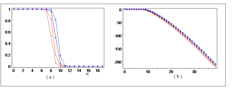 Figure 1
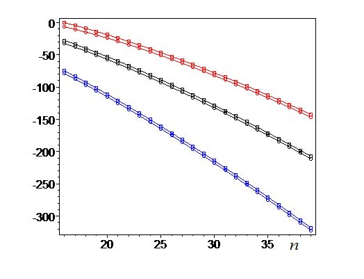 Figure 2
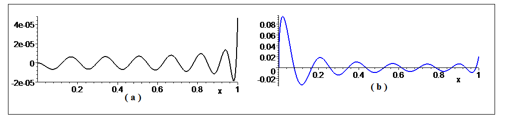 Figure 3
Peer Reviews
No public reviews on file for this paper yet. If you reviewed it on a platform where reviews are public (OpenReview, ICLR, NeurIPS, ICML), you can paste yours below so the community can read it here.
Videos
No videos yet. Explain this paper in a talk, walkthrough, or lecture? Add one.
Taxonomy
TopicsMathematical functions and polynomials · Spectral Theory in Mathematical Physics · Mathematical Analysis and Transform Methods
The finite Hankel transform operator: Some explicit and local estimates of the eigenfunctions and eigenvalues decay rates.
Mourad Boulsane and Abderrazek Karoui 111 Corresponding author: Abderrazek Karoui, Email: [email protected] This work was supported by the DGRST research Grant UR13ES47 and the project CMCU PHC Utique 15G1504.
University of Carthage, Department of Mathematics, Faculty of Sciences of Bizerte, Jarzouna, 7021, Tunisia.
Abstract— For fixed real numbers the finite Hankel transform operator, denoted by is given by the integral operator defined on with kernel To the operator we associate a positive, self-adjoint compact integral operator Note that the integral operators and commute with a Sturm-Liouville differential operator In this paper, we first give some useful estimates and bounds of the eigenfunctions of or These estimates and bounds are obtained by using some special techniques from the theory of Sturm-Liouville operators, that we apply to the differential operator If and denote the infinite and countable sequence of the eigenvalues of the operators and arranged in the decreasing order of their magnitude, then we show an unexpected result that for a given integer is decreasing with respect to the parameter As a consequence, we show that for the and the have a super-exponential decay rate. Also, we give a lower decay rate of these eigenvalues. As it will be seen, the previous results are essential tools for the analysis of a spectral approximation scheme based on the eigenfunctions of the finite Hankel transform operator. Some numerical examples will be provided to illustrate the results of this work.
2010 Mathematics Subject Classification. Primary 42C10, 65L70. Secondary 41A60, 65L15.
Key words and phrases. Finite Hankel transform operator, Sturm-Liouville operator, eigenfunctions and eigenvalues, prolate spheroidal wave functions, approximation of Hankel band-limited functions.
1 Introduction
We first recall that for a bandwidth and a real number the circular prolate spheroidal wave functions (CPSWFs), denoted by are the different eigenfunctions of the following finite Hankel transform operator, see for example [15, 19]
[TABLE]
that is
[TABLE]
Here, is the Bessel function of the first type and order We recall that the Hankel transform is defined on by
[TABLE]
Moreover, for the Hankel Paley-Wiener space is the space of functions from having compactly supported Hankel transforms, that is
[TABLE]
Although, in the literature, there exist extensive works devoted to the numerical computation of the CPSWFs and their associated eigenvalues see for example [2, 15, 18, 19], the subject of the explicit estimates and bounds of the as well as the decay rate of the eigenvalues or is still unexplored. Our objective from this work is to provide the reader with some useful explicit local estimates and bounds of the CPSWFs, as well as some explicit lower and upper bounds of the eigenvalues
We first mention that the interest from the study of the eigenfunctions of the finite Hankel transform (CPSWFs) and in general the prolate spheroidal wave functions, comes from the fact they are widely used in various scientific area, such as applied mathematics, physics, engineering, see [9] for some of these concrete applications.
In the pioneer work [19], D. Slepian has shown that the compact integral operator commutes with the following differential operator defined on by
[TABLE]
Hence, is the th order bounded eigenfunction of the operator associated with the eigenvalue that is
[TABLE]
In this work, we take advantage from the commutativity property of the operators and and prove some useful local estimates and bounds of the Note that some estimates and bounds of the classical prolate spheroidal wave functions and their generalized versions, were already given in [5, 16]. Nonetheless, in our present case of the CPSWFs, the techniques used in the previous references have to be modified and combined with new techniques based on the use of the Sturm-Liouville comparison theorem and Butlewski’s theorem. These new techniques are needed in order to handle the extra difficulty caused by the singularity at appearing in the differential operator Also, by using the characterization of the eigenvalues in terms of an energy maximization problem, combined with Griffith’s theorem which is a Paley-Wiener theorem for the Hankel transform, we prove an interesting result that the are decreasing with respect to the parameter As a consequence, and by using the sharp decay rate of the eigenvalues of the finite Fourier transform, given in [6], we give a super-exponential decay rate of the for
This work is organised as follows. In section 2, we give some mathematical preliminaries related to the properties and computation of the CPSWFs. In section 3, we first provide a local estimate for the Then, we give a bound of for The previous results are obtained under the condition that where is the th eigenvalues of the differential operator By using the classical Strurm-Liouville comparison theorem, we prove that passes through when is around In section 4, we give an upper and a lower bound of the super-exponential decay rate of the eigenvalues Finally, in section 5, we provide the reader with some numerical examples that illustrate the different results of this work. Moreover, in this section, we also show that the are well adapted for the approximation of Hankel band-limited and almost band-limited functions.
2 Mathematical preliminaries.
In this section, we first give a brief description of the computation and the decay rate of the series expansion coefficients of the eigenfunctions in an appropriate basis of This basis is given by the orthogonal functions Here, is the Jacobi polynomial of degree and parameters normalized so that Then, we relate the eigenvalues of the compact and positive operator
[TABLE]
to the solutions of a classical energy maximization problem over the Paley-Wiener space given by (4).
Note that thanks to the important commutativity property of the differential and integral operators and D. Slepian has developed in [19], an efficient computational scheme for the as well as for their corresponding eigenvalues and The Slepian scheme for the computation of is given by the following series expansion,
[TABLE]
Here, are the expansion coefficients, given as the eigenvectors a tri-diagonal infinite order matrix. Moreover, by combining the integral equation (2) and the previous expansion, D. Slepian has given the following analytic extension of the over the unbounded interval
[TABLE]
By evaluating the two expansions (8) and (9) at one gets the following expression of the eigenvalues
[TABLE]
In this work, we check that for a fixed positive integer the sequence has a super-exponential decay rate. Consequently, the previous formulae for computing the and their eigenvalues are practical and highly accurate. Note that by using a slightly modified techniques of those used in [19], one can easily check that the expansion coefficients can be computed by solving the following tri-diagonal system
[TABLE]
where
[TABLE]
The previous system can be written in the following eigensystem
[TABLE]
with and
[TABLE]
Also, note that the expansion coefficients are related to by the following relation,
[TABLE]
In fact, from (2), we have
[TABLE]
[TABLE]
By combining the previous two equalities, one gets (15).
It is well known that the eigenvalues of the differential operator satisfy the differential equation
[TABLE]
Since is the th eigenvalue of the differential operator and since for all , then by using the Min-Max principle, the th eigenvalue of the differential operator satisfies the following bounds,
[TABLE]
Next, we briefly check a classical result that the eigenvalues of the integral operator given by (7) are characterized as the solutions of an energy maximization problem over the Hankel Paley-Wiener space In fact, from [[21], p.154], we have
[TABLE]
On the other hand, by using the previous identity and since is self-adjoint, then a straightforward computation, gives us
[TABLE]
where the kernel is given by (19). On the other hand, since the Hankel transform operator is its own inverse and since by Plancherel formula, we have for
[TABLE]
then, for we have
[TABLE]
A standard result about the maximization of a quadratic form tells us that the solution of the energy maximization problem
[TABLE]
is given by the first eigenfunction, with the largest eigenvalue of the operator Since then the eigenfunctions of are also the eigenfunctions of and the eigenvalues of are related to the eigenvalues of by the following rule
[TABLE]
Finally, we should mention that throughout this work, the eigenfunctions are normalized by the following rule,
[TABLE]
3 Some explicit estimates and bounds of the eigenfunctions.
In this paragraph, we give an explicit upper bound of with and To this end, we first show that under some conditions on the maximum of is attained at This is given by the following lemma.
Lemma 1**.**
Let be two real numbers. If and then we have
[TABLE]
Proof: We recall that is a solution of the following differential equation
[TABLE]
with
[TABLE]
Next, consider the auxiliary function defined on by
[TABLE]
By computing the derivative of and then using the identity
[TABLE]
one gets
[TABLE]
Note that
[TABLE]
Hence, by combining (27) and (28), one concludes that is increasing on and consequently,
[TABLE]
which concludes the proof of the lemma.
The following lemma provides us with a useful local estimate of the eigenfunctions
Lemma 2**.**
Under the notation and conditions of the previous lemma, we have for
[TABLE]
Proof: We first consider the auxiliary function defined by where is given by (26). Straightforward computations give us
[TABLE]
Hence, we have
[TABLE]
which concludes the proof of the lemma.
As a consequence of Lemma 1 and Lemma 2, we obtain a bound for the eigenfunctions given by the following proposition.
Proposition 1**.**
Let be two real numbers. If and then we have
[TABLE]
Here, is as given by (30).
Proof: Without loss of generality, we may assume that By integrating (6) over the interval with one gets
[TABLE]
Let be the function defined on by
[TABLE]
It can be easily checked that if then is decreasing and positive in Hence, by using (30) and (31), one gets
[TABLE]
Consequently, we have,
[TABLE]
In a similar manner as it is done in [5], let with
[TABLE]
where is a constant to be fixed later on. By combining (32) and (33) and by using the result of lemma 1, one gets
[TABLE]
On the other hand, since for any we have then from (33), we have
[TABLE]
By combining the previous two inequalities, one gets
[TABLE]
To conclude the proof, it suffices to note that the minimum of the quantity is obtained for
To extend the previous result to the case where and the interval is substituted with the whole interval we first need to locate the first positive zero of For this purpose, we use the following Sturm-Liouville comparison theorem, that compares the zeros of the eigenfunctions of two second order differential operators, see for example [[3], page 4]
Theorem 1** **(Sturm Comparison Theorem).
Let be two real continuous functions on the interval and let
[TABLE]
be two ODE with and Then between any two zeros of there exists a zero of
The following proposition gives a location of the first zero of where
Proposition 2**.**
Let be two real numbers. Let be the first positive zero of Then for any integer satisfying we have
[TABLE]
Proof: To prove the previous lower bound, we first note that whenever Moreover, from the equality,
[TABLE]
one concludes that and have the same positive sign around as long as the quantity Straightforward computations show that this is the case when with Consequently, we have
[TABLE]
To prove the upper bound in (35), we use the change of function
[TABLE]
that transforms the differential equation (6) to the following equation for , which has the same zeros as on
[TABLE]
Since then we have Consequently, we have
[TABLE]
Then, we use Sturm Comparison theorem to conclude that the first positive zero of or of lies before the second zero of the bounded solution of the differential equation,
[TABLE]
It is well known that the bounded solution of the previous differential equation is given by
[TABLE]
Note that since is a first zero of and since from [10], see also [11], an upper bound of the th positive zero of the Bessel function is given by
[TABLE]
Consequently, by using the Sturm comparison theorem applied to the equations (38) and (39), one concludes that the first positive zero of or of lies before
[TABLE]
which concludes the proof of the proposition.
By using the results of proposition 1 and proposition 2, we get the following theorem that provides us with a bound for which is valid for any
Theorem 2**.**
let and be such that Then, for any positive integer with and where is given by (35), we have
[TABLE]
Proof: We first recall that if then and the inequality (42) follows from proposition 1. Hence, it suffices to consider the case where For this purpose, we use Butlewski’s theorem, regarding the behaviour of the local extrema of the solution of a second order differential equation, see for example [[4], p. 238]. More precisely, if is a solution of the differential equation
[TABLE]
where and are two positive functions belonging to , then the local maxima of is increasing or decreasing, according to the condition that is decreasing or increasing. In our case, we have
[TABLE]
Since
[TABLE]
and since then one can easily check that there exists a unique real number so that the function is increasing in and decreasing in Hence, from Butlewski’s theorem, the local maxima of are decreasing in and increasing in From the proof of proposition 2, we know that the first zero of denoted by is located in where are given by (35). Hence, by integrating (36) over the interval where and then using Hölder’s inequality, one gets
[TABLE]
On the other hand, from the expression of one can easily check that this later is positive whenever Consequently, we have
[TABLE]
By using the expression of as well as the conditions on together with Hölder’s inequality applied to the above integral, one gets
[TABLE]
Finally, since and since then we have
[TABLE]
Finally, from the previous analysis, we have
[TABLE]
which concludes the proof of the theorem.
The following theorem tells us that passes through for around
Theorem 3**.**
*Consider two real numbers with then,
For any positive integer we have
For any integer we have *
Proof.
To alleviate notation, we let denote the eigenfunction and its associated eigenvalue respectively. We want to prove that solutions on of the differential equation
[TABLE]
have at least zeros. As it is done in the proof of proposition 2, the change of function leads to the equation for , given by (38). Since then from the Sturm comparison theorem, the number of zeros of is bounded below by the number of zeros of the function given by (40). Since a bound of the th zero of the Bessel function is given by (41), then the number of zeros of is bounded below by Finally, to conclude the proof of (a), it suffices to note that and use the previous bound below of the number of zeros
Next to prove (b), we divide the interval into the two subintervals with to be fixed later on. We first bound the number of zeros of or of , in the interval . Since for we have then by using the Sturm-Liouville comparison theorem applied to (44) and the differential equation
[TABLE]
one concludes that
[TABLE]
It remains to find a bound for We now compare the equation (44) with an appropriate second order differential equation on the interval We may assume that Since in this last interval, we have and since and then we have
[TABLE]
Hence, we use the Sturm-Liouville comparison theorem applied to the equation (44) and the following equation
[TABLE]
The previous equation is rewritten as
[TABLE]
If we let and take as a new variable, then the previous equation is reduced to the Bessel equation with solution on , with Moreover, since from [[21], p.489], the th zeros of lies in the interval then has at most zeros in By using Sturm comparison theorem, one concludes that the number of zeros of in is bounded as follows,
[TABLE]
Straightforward manipulations show that
[TABLE]
since then from (18), we have Moreover, by choosing one gets
[TABLE]
that is which allows us to conclude for (b). ∎
4 Eigenvalues behaviour and decay of the finite Hankel transform operator
In this paragraph, we prove an important property of the eigenvalues that is for fixed integer and real numbers we have To prove this result, we need the following Paley-Wiener theorem for the Hankel transform, given by J. L. Griffith in [13].
Theorem 4** ([13]).**
Let and with Let be an even function of exponential type 1. If and then can be represented by
[TABLE]
with Conversely, if has this representation and then is an even entire function of exponential type such that
By using the previous theorem, we prove the following lemma that compares two Paley-Wiener spaces for Hankel band-limited functions. We should mention that the previous theorem is still valid if the the interval is substituted with the interval
Lemma 3**.**
let be two real numbers, then the Hankel Paley-Wiener spaces and satisfy the following inclusion relation,
[TABLE]
Here, is as given by (4).
Proof.
Since then for we have
[TABLE]
It follows that
[TABLE]
Let then . By using the previous Griffith’s theorem with one concludes that the function is an even entire function of exponential type 1. Moreover, since and since then we have
[TABLE]
Again by using Griffith’s theorem, one concludes that there exists a function such that and
[TABLE]
Hence
[TABLE]
It follows from (49) that and That is and ∎
By using the previous lemma, we show that for a fixed integer the eigenvalues is decreasing with respect to the parameter This unexpected result is one of the main results of this work and it is given by the following theorem.
Theorem 5**.**
Let \big{(}\lambda_{n,\alpha}(c)\big{)}_{n\geq 0} be the sequence of the eigenvalues of the operator then for any integer we have
[TABLE]
Proof.
We first recall that if is a self-adjoint compact operator on a Hilbert space with positive eigenvalues arranged in decreasing order, then by Min-Max theorem, we have
[TABLE]
where is a subspace of of dimension In the special case where and by using the discussion given in section 2, that relates the energy maximization problem to the eigenvalues one concludes that
[TABLE]
where the are subspaces of of dimensions . Next, let then by using Lemma 3, we get
[TABLE]
On the other hand, for we have
[TABLE]
which implies that
[TABLE]
That is
[TABLE]
Similarly, for and by using Lemma 3, we get
[TABLE]
Hence, by (51) we get which completes the proof of the theorem. ∎
Note that in the special case where we have and the are the solutions of the eigen-problem
[TABLE]
Moreover, it is well known that the solutions of the previous eigen-problem are given by the classical prolate spheroidal wave functions of odd orders These PSWFs are solutions of the integral equations,
[TABLE]
[TABLE]
From the previous three equalities, one gets the following identity relating the eigenvalues of to the eigenvalues associated to the classical PSWFs of odd orders,
[TABLE]
Note that unlike the eigenvalues the behaviour and the sharp decay rate of eigenvalues associated with the classical PSWFs, are well known in the literature, see for example [6, 12, 17, 20]. In particular, it has been shown in [6] that the sharp asymptotic decay rate of the is given by More precisely, for any real there exists a constant such that for Moreover, for any real there exists a constant such that for By combining the monotonicity of the with respect to the parameter the identity (55) and the previous decay rate of the classical eigenvalues one gets the following corollary that provides us with a super-exponential decay rate of the
Corollary 1**.**
Let and be two positive real numbers. Then for any there exits a constant such that
[TABLE]
Unfortunately and unlike the classical case, we don’t have a precise asymptotic lower decay rate of the Nonetheless, the following proposition gives us a bound below for the asymptotic decay rate of the with a similar type of the super-exponential decay of the bound above.
Proposition 3**.**
Let be a positive real number, then there exists a constant and a positive integer such that for any integer and we have
[TABLE]
for some positive constant
Proof: It is well known, see [19] that satisfies the differential equation,
[TABLE]
Here, we recall that is normalized so that It can be easily checked that in this case, satisfies
[TABLE]
On the other hand, from [1], there exists a positive integer and a positive real number such that
[TABLE]
Since the are arranged in the decreasing order, then the previous inequality implies that for any integer or any Also, by using (58), one gets
[TABLE]
On the other hand, it has been shown in [14] that for and the WKB uniform approximation of the is given by
[TABLE]
where is a normalization constant, is a constant depending only on and
[TABLE]
Also, from [14], we know that in the neighbourhood of the quantity is bounded uniformly in Moreover, by using the same techniques as those used in [8] for the approximation of the normalization constant appearing in the WKB approximation of the classical PSWFs, one concludes that our normalization constants are also bounded uniformly in as soon as Consequently, if we also assume that then using the previous analysis together with the upper bound of given by (18), one concludes that there exists a constant such that
[TABLE]
It is easy to see that the previous inequality is still valid for any Finally, by substituting with in (61) and using (59), one gets the desired result (57).
As a consequence of the previous proposition, we have the following corollary showing the super-exponential decay rate of the does not invalidate an exponential decay of the expansion coefficients given by (15).
Corollary 2**.**
Under the hypotheses on the integer given by the previous proposition, there exist two positive constants such that for any integer we have
[TABLE]
Proof: We first note that the Bessel function satisfies the following bound, see for example [4], Here, denotes the Gamma function. By combining (15) and the previous inequality, one obtains
[TABLE]
The last inequality follows from the Hölder’s inequality applied to the integral On the other hand, it is well known that Consequently, we have
[TABLE]
Finally, by combining the previous inequality and (57) and taking into account that one gets the desired inequality (62).
5 Numerical Results
In this paragraph, we give some numerical examples that illustrate the various results of the previous sections. Moreover, we show that the eigenfunctions of the finite Hankel transform operator are well adapted for the approximation of Hankel- and almost Hankel Band-limited functions.
Example 1: In this example, we illustrate one of the main results of this work, which is given by Theorem 5. That is the eigenvalues are decreasing with respect to the parameter For this purpose, we have considered the values of and the four values of Then, we have used formula (10) and computed highly accurate approximation of the eigenvalues with In Figure 1(a), we have plot the graphs of the significant eigenvalues with the various values of and In order to check that the decay with respect to the parameter holds also for the very small eigenvalues, we have plot in Figure 1(b) the graphs of the Note that the results given by the previous figures indicate what was expected by Theorem 5, that is the are decreasing with respect to the parameter
Example 2: In this example, we give some numerical tests that illustrate the super-exponential decay rate of the eigenvalues given by Corollary 1. For this purpose, we have considered the value of and the three different values of and computed highly accurate values of the eigenvalues for By Theorem 2, these values of correspond to the case where As in the classical case, the critical value of corresponds to the beginning of the plunge region of the eigenvalues In Figure 2, we plot the graphs of the highly accurate values of the as well as the graphs of the logarithm of the optimal theoretical super-exponential decay rate, as given by corollary 1. Note that for the different values of the theoretical asymptotic decay rate given by corollary 1 is very close to the actual decay rate.
Example 3: In this last example, we illustrate the quality of the spectral approximation of the Hankel band-limited and almost Hankel band-limited functions, by the orthogonal projection over Note that the concept of almost band-limited functions has been introduced in the framework of the classical Fourier transform by Landau, see [17]. In a similar manner, the almost Hankel band-limited functions are defined as follows.
Definition 1**.**
Let be a measurable set of and let be a positive real number. A function is said to be almost band-limited to if
[TABLE]
Here denotes the characteristic function of
In particular, since the are Hankel band-limited functions, then they are almost band-limited to Next, for an integer let be the -th partial sum of the expansion of in the basis that is
[TABLE]
where denotes the usual inner product of The quality of approximation of the classical Fourier almost band-limited functions, by the classical PSWFs has been given in [7]. Moreover, in [12], this quality of approximation has been extended to the expansion with respect to some families of classical orthogonal polynomials. By straightforward modifications of the techniques used in [12], one gets the following proposition that provides us with the quality of approximation of almost Hankel band-limited function by the
Proposition 4**.**
If is an function that is almost Hankel band-limited in then for any positive integer we have
[TABLE]
To illustrate the previous spectral approximation result, we have considered the following Hankel and almost Hankel band-limited functions, given by
[TABLE]
respectively. Note that the Hankel transforms of and are given by
[TABLE]
Hence, for any Moreover, straightforward computations show that is concentrated on with
[TABLE]
In the special case where and we have For this last value of we have computed the -th partial sum and with The approximation errors and are given in Figure 3(a) and 3(b), respectively. Note that as predicted by the previous proposition, the first approximation error is proportional to and the second one is proportional to
The reference list from the paper itself. Each links out to its DOI / PubMed record.
- 1[1] L. D. Abreu and A. S. Bandeira, Landau’s necessary conditions for the Hankel transform, J. Funct. Anal. 262 (4), (2012), 1845–1866.
- 2[2] P. Amodio, T. Levitina, G. Settanni and E. B. Weinmüller, On the calculation of the finite Hankel transform eigenfunctions, J. Appl. Math. Comput., 43 (1), (2013), 151–173.
- 3[3] W.O. Amrein, A. M. Hinz and D. B. Pearson, Sturm-Liouville Theory: Past and Present, Birkhäuser, Basel-Boston-Berlin, 2005.
- 4[4] G. E. Andrews, R. Askey and R. Roy, Special Functions, Cambridge University Press , Cambridge, New York, 1999.
- 5[5] A. Bonami and A. Karoui, Uniform bounds of prolate spheroidal wave functions and eigenvalues decay, C. R. Math. Acad. Sci. Paris. Ser. I, 352 (2014), 229–234.
- 6[6] A. Bonami and A. Karoui, Spectral Decay of Time and Frequency Limiting Operator, Appl. Comput. Harmon. Anal. 42 (2017), 1–20.
- 7[7] A. Bonami and A. Karoui, Approximations in Sobolev Spaces by Prolate Spheroidal Wave Functions, Appl. Comput. Harmon. Anal. Doi:10.1016/j.acha.2015.09.001.
- 8[8] A. Bonami and A. Karoui, Uniform approximation and explicit estimates of the Prolate Spheroidal Wave Functions, Constr. Approx. 43 (1), (2016), 15–45.