An Information-Theoretic Analysis of Deduplication
Urs Niesen

TL;DR
This paper offers an information-theoretic framework for analyzing data deduplication, introducing new models and schemes, and demonstrating the near-optimality of a novel multi-chunk approach under mild assumptions.
Contribution
It develops a formal information-theoretic analysis of deduplication, introduces a new multi-chunk scheme, and highlights the importance of boundary synchronization for optimality.
Findings
Multi-chunk deduplication is order optimal under mild conditions.
Boundary synchronization is crucial for deduplication efficiency.
The paper formalizes fixed-length and variable-length deduplication schemes.
Abstract
Deduplication finds and removes long-range data duplicates. It is commonly used in cloud and enterprise server settings and has been successfully applied to primary, backup, and archival storage. Despite its practical importance as a source-coding technique, its analysis from the point of view of information theory is missing. This paper provides such an information-theoretic analysis of data deduplication. It introduces a new source model adapted to the deduplication setting. It formalizes the two standard fixed-length and variable-length deduplication schemes, and it introduces a novel multi-chunk deduplication scheme. It then provides an analysis of these three deduplication variants, emphasizing the importance of boundary synchronization between source blocks and deduplication chunks. In particular, under fairly mild assumptions, the proposed multi-chunk deduplication scheme is…
Click any figure to enlarge with its caption.
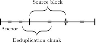 Figure 1
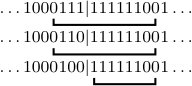 Figure 2
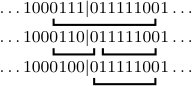 Figure 3
 Figure 4
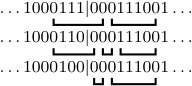 Figure 5
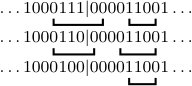 Figure 6
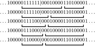 Figure 7
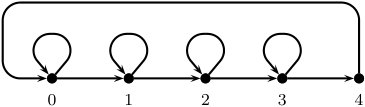 Figure 8
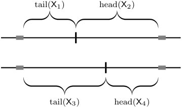 Figure 9
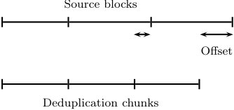 Figure 10
Peer Reviews
No public reviews on file for this paper yet. If you reviewed it on a platform where reviews are public (OpenReview, ICLR, NeurIPS, ICML), you can paste yours below so the community can read it here.
Videos
No videos yet. Explain this paper in a talk, walkthrough, or lecture? Add one.
An Information-Theoretic Analysis of Deduplication
Urs Niesen The author is with Qualcomm’s New Jersey Research Center, Bridgewater, NJ 08807. Email: [email protected] paper was presented in part at IEEE ISIT 2017.
Abstract
Deduplication finds and removes long-range data duplicates. It is commonly used in cloud and enterprise server settings and has been successfully applied to primary, backup, and archival storage. Despite its practical importance as a source-coding technique, its analysis from the point of view of information theory is missing. This paper provides such an information-theoretic analysis of data deduplication. It introduces a new source model adapted to the deduplication setting. It formalizes the two standard fixed-length and variable-length deduplication schemes, and it introduces a novel multi-chunk deduplication scheme. It then provides an analysis of these three deduplication variants, emphasizing the importance of boundary synchronization between source blocks and deduplication chunks. In particular, under fairly mild assumptions, the proposed multi-chunk deduplication scheme is shown to be order optimal.
I Introduction
I-A Motivation
Data deduplication is a commonly used technique to reduce storage requirements in data centers and enterprise servers. It operates by identifying and removing duplicate blocks of data over long ranges. For example, consider a corporate logo used in many slide decks of that corporation. The enterprise storage server, using deduplication, can store only the first occurrence of the logo and replace subsequent occurrences with pointers to the earlier stored one.
The above example highlights key differences between deduplication and algorithms used to compress single files. These latter, by now standard, data compression approaches include DEFLATE [1] (based on LZ77 [2] and used in the popular zlib and gzip utilities) and PPM (prediction by partial match) [3]. They operate by finding small amounts of local redundancy. For example, DEFLATE uses a sliding window and restricts the match length to a maximum of [1] (although the typical match length is likely considerably smaller—on the order of a few tens of bytes). Similarly, PPM typically uses a context of up to [4]. In contrast, data deduplication finds larger amounts of global redundancy. For example, [5] reports finding duplicates on the order of a few up to a hundred over ranges of several hundreds of up to a few . Thus, the main difference between data deduplication and single-file compression is the scale at which they operate.
To deal with this large scale, deduplication algorithms use an approach called chunking. In the simplest version, the stream of data (of size up to several ) is split into chunks of fixed size (say ). The algorithm sequentially processes the stream of chunks. For each chunk, the algorithm computes a hash value, used as key into a hash table. If the hash table does not already contain an entry with that key, the algorithm enters the chunk into the hash table (hash collisions can be avoided by proper dimensioning of the length of the hash value). The chunk is then deduplicated by replacing it with its hash value. The hash table and the sequence of chunk hashes are stored on disk. Since indexing into the hash table can be performed in constant time, this chunking approach is computationally efficient and can be performed over large amounts of data.
This fixed-length chunking has the disadvantage that it is susceptible to shifts of the duplicate data blocks. Returning to the corporate logo example, if the positions of the logo in the data stream are not aligned with respect to the chunk boundaries, then duplicates will not be discovered. To address this issue, most deduplication systems instead use variable-length chunking, in which the chunk boundaries are defined by the occurrence in the data stream of short pre-defined anchor sequences. The chunks now have variable random length. By choosing the length of the anchor sequence, the expected length of the chunks can be controlled. The use of anchor sequences “resynchronizes” the appearance of shifted redundant data blocks, allowing to successfully deduplicate them.
Deduplication has received significant amounts of attention in the Computer Systems literature, as surveyed in Section I-C. It is also widely used in practice; for example, it is reportedly being used both by Dropbox [6] and by Microsoft Windows Server 2012 [5]. Despite its significance, data deduplication seems not to have been studied from a theoretical point of view. In particular, an information-theoretic analysis of its performance limits is missing.
I-B Summary of Contributions
This paper provides such an information-theoretic analysis of data deduplication. The main results of this paper are as follows:
- •
It introduces a simple source model, which captures the long-range memory and the synchronization issues observed in the data deduplication problem.
- •
It formalizes concise versions of the two standard data deduplication approaches, one with fixed chunk length and one with variable chunk length. It also proposes a third, novel, multi-chunk deduplication scheme.
- •
It analyzes the performance of these three schemes. The fixed-length deduplication scheme is shown to be close to optimal when the source-block lengths are constant and known a-priori. However, when the source-block lengths are variable, fixed-length deduplication is shown to be substantially suboptimal. The reason for this suboptimality is formally shown to be due to the lack of synchronization between source block and deduplication chunk boundaries.
- •
The variable-length deduplication scheme is shown to better handle this lack of synchronization. Careful choice of anchor sequence length (or, equivalently, expected deduplication-chunk length) is shown to be critical for good performance of variable-length deduplication.
- •
Finally, the proposed multi-chunk deduplication scheme is shown to be much less sensitive to the expected deduplication chunk length. As a consequence, it can better adapt to the source statistics, and has order-optimal performance under fairly mild conditions.
I-C Related Work
The use of variable-length chunking for the purpose of detecting similar files in large file systems was proposed in [7]. Deduplication based on this variable-length chunking idea was proposed in [8] in the context of a network file system.
The largest gains of data deduplication are achieved when storing different versions of the same data such as in archival storage [9, 10] and backup systems [11, 12, 13]. However, data deduplication has also been successfully applied to primary storage systems [14, 5]. A further area of application is virtual machine hosting centers, where data deduplication is used for virtual machine migration [15] and for virtual machine disk image storage [16].
As already mentioned, data deduplication has not yet been investigated from an information-theoretic point of view. The closest problems in the information theory literature are compression with unknown alphabets [17], also known as multi-alphabet source coding [18, 19], or the zero-frequency problem [4]. In fact, the large repeated blocks in the source data can be interpreted as being part of an unknown alphabet that has to be learned and described by the encoder.
The related problem of file synchronization has been studied extensively in the information-theoretic literature [20, 21, 22, 23, 24, 25, 26]. The synchronization problem is concerned with duplicates between two versions of the same file. In contrast, deduplication deals with a large number of duplicated files or data blocks, and the correspondence between them is not known a-priori.
I-D Organization
The remainder of this paper is organized as follows. Section II provides a formal definition of the problem setting, including the source model and the deduplication schemes. Section III presents the main results. Section IV contains concluding remarks. All proofs are deferred to appendices.
II Problem Setting
II-A Source Description
In order to enable an information-theoretic analysis of data deduplication, we introduce a clean source model. As was pointed out in Section I-A, the data in deduplication problems exhibits global long-range dependency: large blocks of data that are replicated across the entire source sequence. Further, it is unknown a-priori what and where these repeated blocks are. Rather the deduplication algorithm, having access to only the source sequence of zeros and ones, has to discover and then describe any repeated blocks. Finally, the sizes of the repeats differ from block to block and are not known a-priori.
We start with a high-level description of the source model. The source generates a single binary source sequence . This source sequence is the concatenation (without any commas or other delimiters) of source blocks, each of which is itself a binary sequence. These source blocks are chosen independently and uniformly at random from a source alphabet. This source alphabet is generated at random and consists of randomly chosen binary sequences of variable length. The goal is to compress the source sequence knowing neither the source alphabet nor the parsing into the source blocks.
We next provide a formal description of the source model. We consider a source alphabet , of size , generated randomly as follows. Fix a distribution over with finite mean . Generate independently and identically distributed (i.i.d.) random variables from . We next generate a sequence of binary strings for each : Starting with , choose uniformly at random from . Thus, each is a binary string of length , called a source symbol in the following. Finally, the source alphabet (where denotes the set of all finite-length binary sequences) is defined as the union of all the source symbols,
[TABLE]
Note that is equal to since the are drawn without replacement. To simplify some of the derivations later on, we assume that is tightly concentrated around its mean, specifically that \mathbb{P}\bigl{(}\mathbb{E}(\mathsf{L})/2\leq\mathsf{L}\leq 2\mathbb{E}(\mathsf{L})\bigr{)}=1. Furthermore, to ensure that the source alphabet generation is always well defined, we assume that .111Since , the assumption would be sufficient for the source model (in which the source symbols are drawn without replacement) to be well defined. The additional term is added to simplify the derivations later on.
From this randomly generated source alphabet , we now choose elements i.i.d. uniformly at random. Each is referred to as a source block. Recall that each source symbol is an element of . Since each source block is equal to a randomly chosen source symbol, it is therefore also an element of , i.e., a binary sequence of variable length.
Finally, we construct the random source sequence as the concatenation of . We emphasize that is an element of , in other words, the boundaries of the source blocks are not preserved. Denote by the (random) length of .
Example 1**.**
Assume the source alphabet is randomly generated to contain the source symbols . From this, source blocks are drawn i.i.d. uniformly at random, say and . The resulting source sequence is then .
Our goal is to compress the source sequence , knowing only , , and . In particular, the source alphabet and the parsing into the source blocks are not known. More formally, we are looking for a prefix-free source code for the random variable . We have a complete statistical description of and (since is finite) its entropy is well defined. The expected rate of the optimal prefix-free source code for is thus bounded as
[TABLE]
Example 2**.**
We illustrate the order and relative size of the various quantities in the problem setting using data from a recent large-scale primary (i.e., non backup) data deduplication study [5]. The length of the source sequence ranges from several hundreds of to a few . The expected value of the length of the source symbols is a bit harder to quantify (since the notion of source symbol itself is a model abstraction), but the experiments in [5] suggest that reasonable numbers range from a few to a few . The number of source blocks is consequently on the order of perhaps to . As in our model, the data in [5] indicates that duplicates are not localized, but occur over the entire source sequence. In other words, the source has long-range dependence. The number of distinct source symbols is again hard to precisely quantify. Experimental results in [5, 12] indicate that, depending on the scenario, most duplicates occur no more than around times. This suggests that should be somewhere in the range to .
There are two key differences between the source model introduced here and the standard source coding setup.
First, the standard setting is to consider the source statistics, captured by and , as fixed and to let the length of the source, captured by , go to infinity. Instead, as indicated by Example 2, we are interested here in the regime when may be of similar order as . Thus, we here allow the source parameters and to grow with .
Second, given the size of the problem and in particular the long range over which the source exhibits memory (see again Example 2), we are interested in compression schemes that scale well. As mentioned in Section I, it is this scaling requirement of removing large amounts of redundancy (hundreds of ) over long ranges (hundreds of ) that preclude the use of standard compression algorithms such as LZ77 [2]. Instead, we next describe three deduplication schemes that do scale well.
II-B Deduplication Schemes
We next provide a formal (somewhat stylized) description of the deduplication approach. There are two types of deduplication schemes that appear frequently in the literature, fixed-length and variable-length, which are presented first. Then, we introduce a novel variant of the deduplication approach, termed multi-chunk deduplication.
For fixed-length deduplication, we fix a chunk length . The source sequence is parsed into substrings of length (except for the final substring that may have length less than ). Let be this fixed-length parsing of with . Each (with ) is an element of referred to as a deduplication chunk.
The encoding algorithm starts by describing the length of the source sequence using a prefix-free code for the positive integers (such as an Elias code [27]). The encoding algorithm then traverses through the chunks, starting at , and constructs a growing dictionary of chunks seen up to . Chunk is encoded either as a new dictionary entry or as a pointer into the dictionary at that point (depending on whether the chunk is new or already in the dictionary). If chunk is new, then it is encoded as the bit followed by the binary string itself. If chunk is not new, then it is encoded as the bit [math] followed by a pointer into the dictionary. This fixed-length deduplication scheme is prefix free. Its expected (with respect to ) number of encoded bits is denoted by .
Example 3** (continues=eg:setting).**
Continuing with Example 1, for and with , the fixed-length chunks are , , , . When the encoding process terminates, the chunk dictionary contains the elements .
The encoding of the source sequence length is (using an Elias gamma code). The first two chunks and are not in the dictionary and are therefore encoded as and , respectively. At this point in the encoding process, the dictionary is . Chunk is equal to the first chunk in the dictionary, and is encoded as (the first [math] indicating that the chunk is not new and the second [math] indicating the position in the dictionary using bits). The last chunk is new and is encoded as . The complete encoded source sequence using fixed-length deduplication is the concatenation of the various encoded chunks and equal to .
The decoder decodes this encoded source sequence by first reading and decoding the source sequence length to . Knowing the value of , it then traverses the encoded source sequence, decoding each chunk and building the dictionary in the process.
Remark 1*:*
Without the initial encoding of , the source code is still nonsingular (i.e., no two different have the same encoding), and can hence be decoded. However, because of the variable-length nature of the source, the code may no longer be prefix free. (For example, using fixed-length deduplication with , the source sequence [math] would be encoded as and the source sequence as .) The initial encoding of is therefore necessary to guarantee that the source code is prefix free.
For variable-length deduplication, we fix an anchor sequence, which we take here to be the all-zero sequence of length denoted by . The source sequence is then split into a random number of chunks using this anchor. More formally, the source sequence is parsed as , where each chunk (except for perhaps the last one) contains a single appearance of the sequence at the end.
The encoding algorithm again starts by describing the length of the source sequence using a prefix-free code for the positive integers. The encoding of the sequence itself is also performed using a growing dictionary of chunks, similar to the fixed-length scheme. If chunk is new (meaning not yet in the dictionary), it is encoded as the bit followed by the binary string itself. Since the anchor sequence indicates the end of , we do not need to store the length explicitly. If chunk is not new, then it is encoded, as before, as the bit [math] followed by a pointer into the dictionary. This variable-length deduplication scheme is also prefix free. Its expected (with respect to ) number of encoded bits is denoted by .
Example 4** (continues=eg:setting).**
Continuing again with Example 1, for and with , the variable-length chunks are , . When the encoding process terminates, the chunk dictionary contains the elements .
Once the chunking is completed, the remainder of the encoding process for variable-length deduplication is similar to fixed-length deduplication. The initial encoding of the source sequence length is again . Both chunks and are not in the dictionary and are therefore encoded as and , respectively. The encoded source sequence is the concatenation of the various encoded chunks and equal to .
As for fixed-length deduplication, the decoder decodes this encoded source sequence by first reading and decoding the source sequence length to . Knowing the value of , it then traverses the encoded source sequence, decoding each chunk and building the dictionary in the process. For example, upon seeing the first bit of the remaining encoded source sequence , the encoder knows that the next chunk is new (the initial bit is ). It removes the and reads the encoded sequence until the first occurrence of the anchor , which results in the string is . This is the decoded first chunk, which since it is new is also added to the dictionary.
Example 5** (continues=eg:setting2).**
For a more realistic example, consider again the setting for the primary data deduplication study [5] from Example 2. The system uses variable-length chunking with expected chunk lengths ranging from to . The corresponding anchor sequence has length ranging from to bits. [5] finds that around of chunks appear only once, and that the vast majority of chunks have less than duplicates. It is worth pointing out that the number of duplicates may be higher in backup or archival scenarios, where deduplication ratios of to or higher can be achieved [12].
We finally describe the novel, multi-chunk deduplication algorithm. We again split the source sequence into a random number of chunks using the anchor , however, this time we ensure that each chunk has length at least . More formally, the source sequence is parsed as , where each chunk (except for perhaps the last one) is the shortest string of length at least ending in .
Example 6**.**
Multi-chunk deduplication with anchor length parses the source sequence into the chunks , , .
The encoding algorithm again describes the length of the source string using a prefix-free code for the positive integers, followed by a parsing of using a growing dictionary of chunks. Consider the encoding of chunk . Assume first that it is new, and consider the sequence of chunks. Let be the largest integer such that are all new. These new chunks are then encoded together as the bit , followed by an encoding of using a prefix-free code for the positive integers, followed by the binary string . Since each chunk is terminated by the occurrence of the anchor sequence after position , we do not need to store their lengths explicitly. The encoding process continues with chunk .
Assume next that chunk is not new, and consider the sequence of chunks. Let be the smallest index satisfying . Such an index exists since chunk is not new; in fact corresponds to the first time chunk was seen and hence entered into the dictionary. Consider the corresponding dictionary entry and the list of subsequent entries. Let be the largest integer such that , , …, is equal to , , …, . Then the chunks through are encoded together as the bit [math], followed by an encoding of using a prefix-free code for the positive integers, followed by a pointer into the dictionary pointing to chunk . Observe that the pointer is to an individual chunk, even if that chunk was part of a larger group of chunks encoded jointly. The encoding process continues with chunk .
This multi-chunk deduplication scheme is also prefix free. Its expected (with respect to ) number of encoded bits is denoted by .
II-C Performance Metric
The standard performance criterion is the redundancy normalized by the expected length of the source sequence, i.e., . However, it can be verified that in our setting itself may be . In these cases,
[TABLE]
which may be small even if and are very different. Thus, the normalized redundancy may not be a meaningful quantity. We therefore instead adopt the ratio (and similar for , ) as our performance metric. This ratio performance metric is strictly stronger than the standard normalized redundancy performance metric.222Indeed, it is easily seen that
\frac{R-R^{\star}}{\mathbb{E}\ell(\mathsf{S})}=\frac{R^{\star}}{\mathbb{E}\ell(\mathsf{S})}(R/R^{\star}-1)\leq\bigl{(}1+o(1)\bigr{)}(R/R^{\star}-1)
as .
A deduplication scheme with rate is order optimal if as . It is asymptotically optimal if as .
As indicated in Section II-A, while the standard approach is to fix the source alphabet parameters, i.e., and , and to consider the asymptotic behavior as the source length (as measured by ) increases, we are here instead interested in the behavior as the source alphabet parameters increase together with the source length .
III Main Results
The aim of this paper is to provide an information-theoretic analysis of data deduplication for the source model defined in Section II-A. We start with the fixed-length deduplication scheme as described in Section II-B. The first result analyzes the performance of this scheme assuming a constant source-symbol length, i.e., . As we will see, under this strong assumption, fixed-length deduplication is close to optimal.
Theorem 1**.**
Consider the source model with source blocks drawn with replacement from the source symbols of constant length . The performance of the fixed-length deduplication scheme with chunk length satisfies then
[TABLE]
for large enough.333All logarithms are to the base two.
The proof of Theorem 1 is reported in Appendix A. The most interesting regime is when the number of source blocks is at least as large as the number of source symbols , in which case the upper bound in Theorem 1 can be simplified to
[TABLE]
Thus, as long as for some as (which implies that as by assumption), we have that as grows, showing the asymptotic optimality of fixed-length deduplication with known and constant source-symbol lengths
Example 7**.**
Motivated by Example 2, consider the source with symbols of fixed length bits and with source blocks. Theorem 1 shows then that fixed-length deduplication with chunk length has performance satisfying
[TABLE]
i.e., very close to optimal.
Unfortunately, the asymptotic optimality of fixed-length deduplication relies crucially on the assumption of fixed and known source-symbol length. While this assumption may be reasonable in certain scenarios (such as for virtual machine disk image deduplication [16]), it is usually not valid. As soon as this assumption is relaxed, fixed-length deduplication can be substantially suboptimal, as the next example shows.
Example 8**.**
Consider the scenario with source symbols. To start with, assume the source-symbol length is constant, . By Theorem 1, fixed-length deduplication with chunk length is then within a constant factor of optimal as .
On the other hand, assume next that the symbol-length distribution assigns equal mass to the values and with as before. Appendix B then shows that fixed-length deduplication with chunk length has rate satisfying
[TABLE]
as . In other words, even with only two source symbols, the fixed-length deduplication scheme can be substantially suboptimal.
The reason for the bad performance of fixed-length deduplication is that the source blocks and the deduplication chunks are not properly synchronized. Initially, the deduplication chunks are aligned with the source blocks. However, whenever a source block of length is observed, the deduplication chunks shift by one bit with respect to the source blocks (see Fig. 1). Over time, the boundary between deduplication chunks takes on all possible offsets with respect to the source block boundaries. Due to these possible starting points, the fixed-length deduplication scheme encounters distinct chunks instead of the only distinct source symbols, resulting in the factor overhead compared to the optimal scheme. This argument is made precise in Appendix B.
From Example 8, we see that the (general) deduplication problem is fundamentally one of synchronizing deduplication chunks with source blocks. Unfortunately, the fixed-length deduplication scheme cannot achieve this synchronization. This motivates the use of the variable-length deduplication scheme, described in Section II-B, which utilizes anchor sequences to achieve this synchronization. The next theorem bounds its performance.
Theorem 2**.**
Consider the source model with source blocks drawn with replacement from the source symbols of expected length . The performance of the variable-length deduplication scheme with optimized anchor length satisfies then
[TABLE]
for large enough.
The proof of Theorem 2 is reported in Appendix C. We illustrate this result with two examples.
Example 9** (continues=eg:running).**
Consider again the scenario with source symbols and with source blocks. This time, the source symbols are not of constant length, but have the same expected length bits as before. Theorem 2 shows then that variable-length deduplication has performance satisfying
[TABLE]
i.e., is within a factor of optimal. By numerically optimizing the value of the anchor length to minimize the upper bound (C) in Appendix C on the rate , this factor can be further reduced to .
Example 10** (continues=eg:sync).**
Consider again the scenario with source symbols with symbol-length distribution assigning equal mass to the values and with . Recall that the fixed-length deduplication scheme had a rate at least order times larger than the optimal scheme:
[TABLE]
On the other hand, by tightening the arguments in the proof of Theorem 2 for the case (see Appendix D), the rate of the variable-length deduplication scheme satisfies
[TABLE]
Thus, variable-length deduplication is only suboptimal by at most a polylogarithmic as opposed to a linear factor in this example. Thus, we see that variable-length deduplication is able to solve the problem of synchronizing source blocks and deduplication chunks, which was the cause of the poor performance of fixed-length deduplication.
The analysis in the proof of Theorem 2 in Appendix C indicates that the optimal choice of the anchor length , governing the expected chunk length of the variable-length deduplication scheme, balances two competing requirements. On the one hand, for each already encountered chunk, we need to encode a pointer into the dictionary. A smaller chunk length increases both the number of chunks that need to be encoded and the size of the pointers. On the other hand, consider chunks covering the boundaries of two source blocks as shown in Fig. 2. These boundary chunks will usually not be contained in the dictionary (since there are such possible boundaries for source symbols), and will have to be encoded directly. Hence, a larger chunk length increases the amount of bits contained in inefficiently encodable boundary chunks. The choice of anchor length in the proof of Theorem 2 splits each source block into an average of about chunks of expected length about , which balances these two detrimental effects.
Unfortunately, even with this optimal choice of anchor length, using deduplication chunks that have lengths of different order than the source blocks can lead to asymptotically significantly suboptimal performance. This is demonstrated with the next example.
Example 11**.**
Consider the scenario with source symbols of constant length . From the preceding discussion, we see that this is the worst-case situation for variable-length deduplication, in which we can expect to see possible different boundary chunks. A slightly tightened version of Theorem 2 (which omits the last term in the denominator using that is constant) together with a lower bound derived in Appendix E, show that then
[TABLE]
as . This statement has two implications: First, it shows that Theorem 2 is tight to within a polylogarithmic factor in for this setting; and second it shows that variable-length deduplication can still be polynomially suboptimal.
The multi-chunk deduplication scheme proposed in this paper circumvents the competing requirements of how to choose the expected chunk length by encoding multiple chunks jointly. This allows to choose the expected chunk length to be quite small, thereby limiting the effect of the boundary chunks, without the penalty of increased number of dictionary pointers. The next theorem bounds the performance of this scheme.
Theorem 3**.**
Consider the source model with source blocks drawn with replacement from the source symbols of expected length . The performance of the multi-chunk deduplication scheme with optimized anchor length satisfies then
[TABLE]
as .
The proof of Theorem 3 is reported in Appendix F. The theorem shows that, under the fairly mild conditions and for some constant , multi-chunk deduplication is within a constant factor of optimal as . Further, if A\leq B\leq o\bigl{(}A\mathbb{E}(\mathsf{L})/\log(A\mathbb{E}(\mathsf{L}))\bigr{)}, then multi-chunk deduplication is asymptotically optimal as .
Example 12** (continues=eg:running).**
Consider again the scenario with source symbols and with source blocks with expected length bits. Theorem 3 (using the explicit constant in the order notation from Appendix F) shows then that multi-chunk deduplication has performance satisfying
[TABLE]
By numerically optimizing the anchor length to minimize the upper bound (47) in Appendix F on the rate , this factor can be further reduced to . Thus, the proposed multi-chunk deduplication scheme is quite close to optimal in this setting.
Example 13** (continues=eg:duplicate).**
Consider again the scenario with source symbols of constant length . Recall that the variable-length deduplication scheme had a rate at least polynomially suboptimal:
[TABLE]
On the other hand, a slightly tightened version of Theorem 3, which omits the last term in the denominator using that is constant, shows that the rate of the multi-chunk deduplication scheme satisfies
[TABLE]
as . Thus, multi-chunk deduplication is order optimal in this case, as opposed to the polynomial loss factor of variable-length deduplication.
IV Conclusion
Motivated by the practical importance of data deduplication schemes but a lack of theoretical results, this paper initiated the information-theoretic analysis of these schemes. In order to enable this analysis, it introduced a clean and tractable source model capturing the long-range memory and large scale encountered in deduplication applications. It then analyzed the two standard deduplication schemes (fixed-length and variable-length). This analysis uncovers both the strength and the weaknesses of both these schemes. The resulting insight was used to construct a new scheme, called multi-chunk deduplication. This new scheme was shown to be order optimal under fairly mild assumptions.
While the description of the three deduplication schemes is general and applies for any source sequence, their performance analysis relies heavily on the specifics of the clean source model introduced in this paper. In practice one does not have the luxury of such a clean source model. However, the operation of the three deduplication schemes in this paper depend only very weakly on the source model. Indeed, only the chunk length or the anchor length need to be chosen. In practice, one would tune these parameters empirically on a representative dataset.
Appendix A Analysis of Fixed-Length Deduplication with Constant Source-Symbol Length (Proof of Theorem 1)
This appendix analyzes the rate of fixed-length deduplication for constant source-symbol length. The length of the source is in this case the constant . Set the deduplication chunk length to be equal to the fixed length of the source blocks. The deduplication chunks are then equal to the source blocks .
We start with an upper bound on the rate of the fixed-length deduplication scheme. The initial encoding of the length using a universal code for the integers takes at most bits (see, e.g., [28, Lemma 13.5.1]). Consider then the encoding of some chunk . The flag indicating if the chunk is already in the dictionary takes one bit. If the chunk is new, then it is added to the dictionary using bits. If the chunk is already in the dictionary, then a pointer into the dictionary is encoded. Let be the dictionary when processing chunk . Then this encoded pointer takes at most bits.
The expected rate of fixed-length deduplication is thus upper bounded by
[TABLE]
where denotes the indicator function, and where we have used that
[TABLE]
Using that , , and , this upper bound can be rewritten as
[TABLE]
where
[TABLE]
denotes the set of all distinct source blocks seen up to block .
We continue with a lower bound on the rate of the optimal code. Since the code is prefix free, its rate is lower bounded as
[TABLE]
(see, e.g., [28, Theorem 5.4.1]). As the source blocks are of constant length, we have
[TABLE]
with
[TABLE]
Each term in the sum on the right-hand side satisfies
[TABLE]
Conditioned on and , the source block is uniformly distributed over . Hence,
[TABLE]
using that for and that by assumption for . This implies that
[TABLE]
Conditioned on and , the source block is uniformly distributed over . Hence,
[TABLE]
[TABLE]
To obtain a more explicit expression, we further lower bound as
[TABLE]
where follows from and from the convexity of and Jensen’s inequality, follows from
[TABLE]
since the are chosen uniformly with replacement from the set of cardinality , and follows from
[TABLE]
and from
[TABLE]
for and
[TABLE]
for .
[TABLE]
Combining this with (A) yields
[TABLE]
For large enough, this can be simplified as
[TABLE]
concluding the proof. ∎
Appendix B Analysis of Fixed-Length Deduplication with Variable Source-Symbol Length (Example 8)
This appendix contains the formal analysis for Example 8. We start with an upper bound on . Since is the rate of the optimal prefix-free code, it is upper bounded as
[TABLE]
(see, e.g., [28, Theorem 5.4.1]). Now,
[TABLE]
Thus,
[TABLE]
We continue with a lower bound on the rate of fixed-length deduplication. We set the chunk length to be equal to . Since the source blocks have lengths either or , the deduplication chunk boundaries may no longer be aligned with the source block boundaries. Define the offset of the current chunk as the distance from the end of that chunk to the start of the next source block (see Fig. 3(a)).
Recall that , and assume for the moment that the source alphabet has one source symbol of length and one of length (this happens with probability ). The evolution of this offset is then governed by a Markov chain with states as depicted in Fig. 3(b). The initial state is [math] and all outgoing edges of a state have uniform probability. Observe that in each state we make a transition to the right (modulo ) with probability at least or stay in the current state with probability at most . Hence, after transitions, we have traversed the chain at least once in expectation.
Consider now the two source symbols and . And assume for the moment that . By the law of large numbers, about of the deduplication chunks will be substrings of (the concatenation of with itself) with high probability for large enough. Consider all possible chunks of length starting with different offsets in . We next argue that with high probability all these different chunks are unique.
By [29, Example 10.5], there are
[TABLE]
binary sequences of length for which all circular shifts are distinct (these are called aperiodic necklaces in Combinatorics), where is the Möbius function (see, e.g., [29, p. 92] for a definition). Since and , we can lower bound this as
[TABLE]
This shows that, as , the vast majority of binary sequences have the property that all their circular shifts are distinct. In particular, with high probability will have this property.
Putting these arguments together, we obtain the following. With probability the two source symbols have distinct lengths. With probability at least , the shorter of the two source symbols (the one with length ) will have distinct circular shifts for large enough. If and large enough, then we will see every possible deduplication chunk offset at least once with probability at least . Moreover, with probability at least of the deduplication chunks will contain circular shifts of the shorter source symbol. Since each of these are distinct, they will all have to be entered into the dictionary, using bits each. Thus,
[TABLE]
Combining (10) (with and ) and (11) shows that
[TABLE]
as claimed. ∎
Appendix C Analysis of Variable-Length Deduplication (Proof of Theorem 2)
We start with an upper bound on the rate of variable-length deduplication. The initial encoding of the length using a universal code for the integers takes at most bits (see again [28, Lemma 13.5.1]). Consider then the encoding of chunk . The flag indicating if the chunk is already in the dictionary takes one bit. If the chunk is new, then it is added to the dictionary using bits. If the chunk is already in the dictionary, then a pointer into the dictionary is encoded. Let again be the dictionary when encoding chunk . Then this encoded pointer takes at most bits.
Let be the rate of variable-length deduplication for a particular source sequence , so that R_{\mathsf{VL}}=\mathbb{E}\bigl{(}R_{\mathsf{VL}}(\mathsf{S})\bigr{)}. The rate is then upper bounded by
[TABLE]
Now, we have two distinct parsings of the source sequence . The first is defined by the source blocks, ; the second is defined by the deduplication chunks . We would like to relate these two parsings. To this end, let denote the indices of those chunks from starting in . We say that a chunk is in if .
Example 14**.**
Consider , , so that the source sequence is . The parsing of into chunks with anchor yields , , , , , . This situation is depicted in Fig. 2 in Section III. In this setting , , and .
Consider the chunks in source block . As Fig. 2 in Section III shows, some of them depend on the values of the neighboring source blocks and . We call these the “boundary” chunks of and denote their indices by . Other chunks in are the same irrespective of the values of the neighboring source blocks. We call these the “interior” chunks of and denote their indices by . Formally, for a source block , we say that with is an interior chunk if it appears in the variable-length chunking of every sequence with . Any chunk that is not an interior chunk is defined to be a boundary chunk. By definition, the interior chunks thus have the property that if , then . Note that this last conclusion does generally not hold for and .
Example 15** (continues=eg:anchors).**
In this setting we have , , and , , .
Usually, contains only one chunk index, which corresponds to the final chunk starting in but ending in (see Figs. 4(a) and 4(b)). However, can contain additional chunk indices. In particular, if the boundary between and forms an anchor sequence, then the first chunk starting in may also be a boundary chunk (see Figs. 4(b)–4(e)). Finally, if starts with between and zeros (where is the anchor length), then it may contain a third boundary chunk consisting of the anchor sequence by itself (see Fig. 4(d)). Observe that when starts with or more zeros, then there is always a chunk, irrespective of the value of , and therefore is not a boundary chunk in this case (see Fig. 4(e)). In general, we thus have . We will later choose such that as , in which case the vast majority of indices in will correspond to interior chunks.
Let us return to the upper bound (C) for , and consider the first sum corresponding to new chunks. We can now rewrite this sum as
[TABLE]
As before, denote by the set of all distinct source blocks seen up to block as defined in (2) in Appendix A. Note that if for any , then . Hence
[TABLE]
where we have used that
[TABLE]
Substituting this into (C) yields
[TABLE]
Consider then the second sum in (C) corresponding to old chunks. We can upper bound this sum as
[TABLE]
Substituting (14) and (15) into (C) yields
[TABLE]
Taking expectations on both sides results in an upper bound on :
[TABLE]
We now upper bound each of these expectations in turn.
The first expectation in (C) is upper bounded as
[TABLE]
using Jensen’s inequality.
For the second expectation in (C), observe that the number of chunks starting in source block is at most plus the number of times the anchor appears in alone (see again Fig. 2 in Section III). Since the expectation of that latter number is upper bounded by , we obtain
[TABLE]
The third expectation in (C) is equal to
[TABLE]
where we have used the independence of and .
Consider next the fourth expectation
[TABLE]
in (C). Consider the boundary chunks arising at the boundary between and (see again Fig. 4). The total number of bits due to those chunks is upper bounded by the sum of two terms: The number of bits from the end of backwards until the end of the first (counting backwards) occurrence of (or if no such match exists in ). Plus the number of bits from the start of forwards until the end of the first (counting forwards) occurrence of (or if no such match exists in ).
Note that a source symbol is (by itself) a process of random length. The expected value of the end of the first occurrence of in an infinite-length process is by [30, Theorem 8.3]. The expected value of the end of the first occurrence of in an infinite-length process is by [30, Theorem 8.2]. Hence
[TABLE]
In this bound, the event that some source blocks may not contain an anchor sequence is captured by the event that the match of the anchor sequence in the infinite-length process is beyond the length of the corresponding source block.
Consider then the last expectation
[TABLE]
in (C). We have
[TABLE]
Using this, we can upper bound
[TABLE]
where we have used (18).
Substituting (17)–(21) into (C) results in
[TABLE]
We next derive a lower bound on . As before, we have
[TABLE]
Now,
[TABLE]
The term can be bounded as
[TABLE]
using . The term can be bounded similarly to (A) in Appendix A as
[TABLE]
with
[TABLE]
Conditioned on , , and , the source block is uniformly distributed over . Hence,
[TABLE]
where we have used the independence of and the event . Using the assumption that , this last expression can be further lower bounded as
[TABLE]
so that
[TABLE]
Furthermore, by the same arguments as in (A) in Appendix A,
[TABLE]
where the last line follows from Jensen’s inequality.
[TABLE]
To obtain a more explicit expression, we can further lower bound as
[TABLE]
[TABLE]
The two dominant terms in this last expression behave (to first order) like and . Hence, the right-hand side of (C) is approximately minimized by choosing the anchor length as
[TABLE]
This splits each source block into an average of about chunks of expected length about . With this choice of , (C) yields
[TABLE]
where the last inequality holds for large enough. Combining this with (31) yields
[TABLE]
again for large enough. This proves the theorem. ∎
Appendix D Analysis of Variable-Length Deduplication for (Example 8)
The bound (20) in Appendix C is appropriate when . When , it can be quite loose, since each pair yields at most three distinct boundary deduplication chunks. We next derive a tighter bound for the regime .
Define the event that at least one source symbol does not contain the substring . Then, since each pair yields at most three distinct boundary deduplication chunks, we have on the complement of that
[TABLE]
where is the string starting from the beginning of up to and including the first occurrence of , and where is the string from the end of backwards until the end of the first (counting backwards) occurrence of (see Fig. 4 in Appendix C). On , we have
[TABLE]
Combining these last two inequalities yields
[TABLE]
We have
[TABLE]
where we have again used [30, Theorems 8.2 and 8.3]. It remains to analyze . Since by assumption, the probability of the event is upper bounded by that of the event that from sequences drawn uniformly at random without replacement from at least one of them contains no occurrence of . The probability of this last event is upper bounded as
[TABLE]
Hence,
[TABLE]
Substituting (17)–(19), (21), and (33) into (C) in Appendix C yields
[TABLE]
Combined with (30), this shows that
[TABLE]
For the remainder of the argument, we specialize to the setting in Example 8, namely , , . With this, (D) becomes
[TABLE]
Set the anchor length to
[TABLE]
which results in
[TABLE]
Now, since there are only source symbols of length or , we can with high probability uniquely identify the source blocks from for large enough. Hence, each source block adds asymptotically one bit of information to , i.e.,
[TABLE]
as . Combining this with (35) shows that
[TABLE]
as claimed. ∎
Appendix E Analysis of Example 11
Recall that and . Following the same steps as those leading to (10) in Appendix B, we obtain the upper bound
[TABLE]
for the rate of the optimal source code.
We continue with a lower bound on the rate of variable-length deduplication. For each chunk , the flag indicating if the chunk is already in the dictionary takes one bit, resulting in a total of bits. Further, each unique boundary chunk needs to be stored in the dictionary. We next argue that we will see on the order of unique boundary chunks that each have length on the order of . This will imply that storing the unique boundary chunks takes on the order of bits.
Consider the two concatenations of source symbols and , and consider the two resulting boundary deduplication chunks (see Fig. 5). We can decompose the two boundary chunks as the concatenation and , where and denote the substring of the source symbol contributing to the boundary chunk (excluding the anchor sequence, and truncated to length in case there is no anchor sequence before then). From Fig. 5 we see that if , then one of , is a substring of the other, and one of , is a substring of the other.
Consider a source symbol , and assume for now. With probability at least
[TABLE]
it has of length at least and containing a least one symbol in the first bits, and it has of length at least and containing a least one symbol in the last bits. A short calculation (using Markov’s inequality) shows that this implies that with probability at least , the source alphabet has at least symbols with this property.
Moreover, with probability at least the source alphabet has no repeating, nonoverlapping substrings of size . This argument is reported with more detail in Appendix F. In particular, if
[TABLE]
then with probability at least the source alphabet has no repeating, nonoverlapping substrings of size .
Combining the two arguments shows that with probability at least there are at least source symbols with both long, duplicate-free heads and tails. Further, each of these heads contains a symbol one within the first bits, and each of these tails contains a symbol one within its first bits. If this event holds, then of all possible concatenations produce unique boundary chunks of length at least .
Finally, since , we will see at least of these possible unique boundary chunks in expectation. Therefore, the expected number of bits needed to store just the boundary chunks is at least \Omega\bigl{(}\min\{2^{M},L\}B\bigr{)}\geq\Omega\bigl{(}\min\{2^{M},B^{1/2}\}B\bigr{)}, assuming (37) is satisfied.
Combining these arguments, the rate of variable-length deduplication is lower bounded as
[TABLE]
The expected number of chunks is lower bounded by , so that
[TABLE]
This lower bound is minimized by
[TABLE]
which results in the bound
[TABLE]
as .
[TABLE]
as . ∎
Appendix F Analysis of Multi-Chunk Deduplication (Proof of Theorem 3)
We start with an upper bound on the rate of multi-chunk deduplication. The initial encoding of the length using a universal code for the integers takes again at most bits by [28, Lemma 13.5.1]. Consider then the encoding of chunk . The flag indicating if the chunk is already in the dictionary takes one bit. If the chunk is new, then is encoded using at most bits, plus the chunks starting at are added to the dictionary using \ell\bigl{(}\mathsf{Z}_{c}\mathsf{Z}_{c+1}\cdots\mathsf{Z}_{c+\mathsf{V}_{c}-1}\bigr{)} bits. If the chunk is already in the dictionary, then is encoded using at most bits, plus a pointer into the dictionary using at most bits, where is again the dictionary when encoding chunk . The next chunk to be encoded is either or .
As before, we denote by those chunks starting in source block . We again define the notion of boundary chunk indices and interior chunk indices (see Appendix C), but this time with respect to the multi-chunk deduplication scheme, as shown in Fig. 6.
Let be the event that there is at least one interior chunk of that is either equal to another interior chunk in the source alphabet or to a boundary chunk of . Assume we are on the complement of for now, and consider the first interior chunk in (i.e., the smallest ). Then there are two possibilities, either and all indices correspond to new chunks, or and all indices correspond to chunks already in the dictionary.
In the former case (), the number is larger than or equal to . The encoding of the chunks with indices in takes thus at most
[TABLE]
bits. Since reducing the number of jointly encoded chunks and encoding them separately increases the aggregate rate, we can upper bound the total rate by assuming that . The encoding for the first interior chunk in takes in this case at most
[TABLE]
bits.
In the latter case (), the number is larger than or equal to (since the corresponding chunks must have been seen in sequence by the uniqueness assumption), and all the chunks with indices in are encoded together, taking at most
[TABLE]
bits. Again, reducing the number of jointly encoded chunks and encoding them separately increases the aggregate rate, and thus we can upper bound the total rate by assuming that . The encoding for the first interior chunk in takes in this case at most
[TABLE]
bits.
Assume next that we are on . If an interior chunk is not in the dictionary, it is encoded in the worst case using bits. If an interior chunk is in the dictionary, then the pointer into the dictionary takes at most 1+\log\bigl{(}2B\mathbb{E}(\mathsf{L})\bigr{)} bits. In the worst case, each old chunk is encoded separately, leading to an additional bits for the encoding of . Thus, as long as
[TABLE]
the encoding of each old interior chunk takes at most
[TABLE]
bits, since each chunk has length at least by construction. Thus, on the complement of and assuming (39) is satisfied, the encoding of the interior chunks of takes at most
[TABLE]
bits.
Similarly, as long as the condition (39) is satisfied, the boundary chunks can be encoded using at most bits each, regardless of whether they are in the dictionary.
We can then upper bound the rate for a particular source sequence as
[TABLE]
where the second inequality follows after some algebra using the bounds , , and . Taking expectations yields
[TABLE]
It remains to upper bound the last two terms in (F).
For the second-to-last term in (F), we have the upper bound
[TABLE]
Here, are the bits from the start of forward until the end of the first (counting forwards) occurrence of the string such that does not contain . And are the bits from the end of backwards until the end of the first (counting backwards) occurrence of the string plus an additional bits. If no such substring occurs, head and tail denote all the bits in in either case.
The expected value of \ell\bigl{(}\operatorname{tail}(\mathsf{Y}_{b})\bigr{)} is upper bounded as
[TABLE]
as before by [30, Theorem 8.2] (see again Appendix C). The quantity \mathbb{E}\ell\bigl{(}\operatorname{head}(\mathsf{Y}_{b})\bigr{)} can be upper bounded by replacing with an infinite-length process. The head of that Bernoulli process is then a concatenation of sub-chunks of the form with for and with . Consider the sequence of lengths , , …. This sequence forms an i.i.d. stochastic process, and is a stopping time with respect to this process. Thus, we can apply Wald’s equation together with [30, Theorem 8.2] to obtain
[TABLE]
The random variable is geometrically distributed with probability of success lower bounded by . Thus and
[TABLE]
The same argument also shows that
[TABLE]
Substituting (42)–(44) into (41), we obtain
[TABLE]
For the last term in (F), we need to upper bound the probability that there is at least one interior chunk in the source alphabet that is either equal to another interior chunk of the source alphabet or to a boundary chunk of the source sequence. Since all chunks have length at least by construction, whenever this last event holds, then contains a nonoverlapping duplicate substring of length (where the additional factor accounts for the boundary chunks).
Consider a source symbol, say . The probability that it contains a nonoverlapping duplicate substring of length is upper bounded by the probability that a process of length contains such a substring. Consider next two source symbols, say and . Condition on their lengths and . If these lengths are distinct, then and are independent processes of given length. If the lengths are the same, then and are not independent, since they are chosen without replacement. However, the probability of containing a duplicate substring of length from is upper bounded by drawing them with replacement. Further, in both cases, the probability of the event under consideration is increased if we increase the length of the source symbols. In summary, the probability that the source alphabet contains a nonoverlapping duplicate substring of length is upper bounded by the probability that independent processes of length contain such a duplicate. This probability can in turn be upper bounded by \bigl{(}2A\mathbb{E}(\mathsf{L})\bigr{)}^{2}2^{-2^{M-2}}. Therefore,
[TABLE]
Substituting (45) and (46) into (F) yields
[TABLE]
Combined with (30) in Appendix C, this shows that
[TABLE]
Assume first that , and set
[TABLE]
Note that
[TABLE]
satisfying (39). With this choice of , (47) becomes after some simplification
[TABLE]
Assume next that , and set
[TABLE]
Note that then
[TABLE]
again satisfying (39). With this choice of , (47) becomes after some simplification
[TABLE]
From (48) and (49), we conclude that, regardless of the relationship of , , and , we have
[TABLE]
as . Together with (31) in Appendix C, we obtain
[TABLE]
as . ∎
Acknowledgments
The author thanks M. A. Maddah-Ali for helpful initial discussions and the reviewers for their comments.
The reference list from the paper itself. Each links out to its DOI / PubMed record.
- 1[1] P. Deutsch, “DEFLATE compressed data format specification,” RFC 1951, May 1996.
- 2[2] J. Ziv and A. Lempel, “A universal algorithm for sequential data compression,” IEEE Trans. Inf. Theory , vol. 23, pp. 337–343, May 1977.
- 3[3] J. G. Cleary and I. H. Witten, “Data compression using adaptive coding and partial string matching,” IEEE Trans. Commun. , vol. 32, pp. 396–402, Apr. 1984.
- 4[4] I. H. Witten and T. C. Bell, “The zero frequency problem: Estimating the probabilities of novel events in adaptive text compression,” IEEE Trans. Inf. Theory , vol. 37, pp. 1085–1094, July 1991.
- 5[5] A. El-Shimi, R. Kalach, A. Kumar, A. Oltean, J. Li, and S. Sengupta, “Primary data deduplication-large scale study and system design,” in Proc. USENIX ATC , pp. 1–12, June 2012.
- 6[6] I. Drago, M. Mellia, M. M. Munafò, A. Sperotto, R. Sadre, and A. Pras, “Inside Dropbox: Understanding personal cloud storage services,” in Proc. ACM IMC , pp. 481–494, Nov. 2012.
- 7[7] U. Manber, “Finding similar files in a large file system,” in Proc. USENIX TC , pp. 1–10, Jan. 1994.
- 8[8] A. Muthitacharoen, B. Chen, and D. Mazières, “A low-bandwidth network file system,” in Proc. ACM SOSP , pp. 174–187, Oct. 2001.