Emergent Gravity in Spaces of Constant Curvature
Orlando Alvarez, Matthew Haddad

TL;DR
This paper develops a multipole expansion for energy in constant curvature spaces, linking geometric invariants of submanifolds to emergent gravity phenomena, especially in anti de Sitter space.
Contribution
It generalizes a Weyl-based formula to spaces of constant curvature, providing a framework for emergent gravity from embedded submanifolds in quantum field theories.
Findings
Derived a finite multipole expansion for energy in curved spaces
Connected geometric invariants to emergent gravitational constants
Discussed implications for cosmological constant and Planck mass
Abstract
In physical theories where the energy (action) is localized near a submanifold of a constant curvature space, there is a universal expression for the energy (or the action). We derive a multipole expansion for the energy that has a finite number of terms, and depends on intrinsic geometric invariants of the submanifold and extrinsic invariants of the embedding of the submanifold. This is the second of a pair of articles in which we try to develop a theory of emergent gravity arising from the embedding of a submanifold into an ambient space equipped with a quantum field theory. Our theoretical method requires a generalization of a formula due to by Hermann Weyl. While the first paper discussed the framework in Euclidean (Minkowski) space, here we discuss how this framework generalizes to spaces of constant sectional curvature. We focus primarily on anti de Sitter space. We then discuss…
Click any figure to enlarge with its caption.
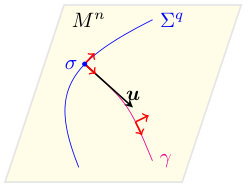 Figure 1
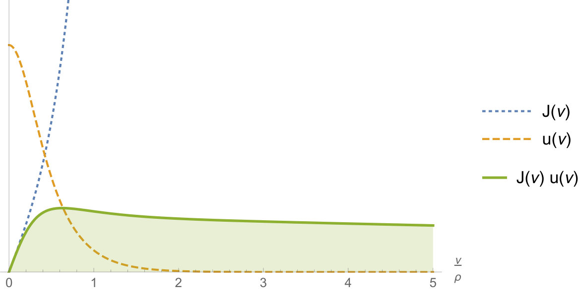 Figure 2
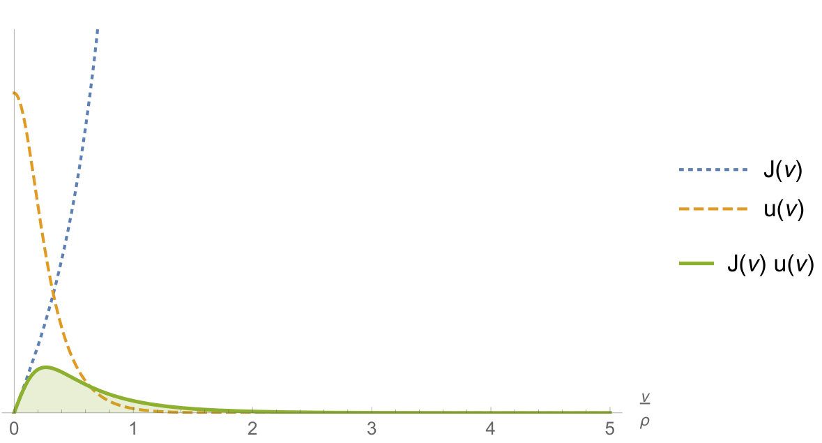 Figure 3
Peer Reviews
No public reviews on file for this paper yet. If you reviewed it on a platform where reviews are public (OpenReview, ICLR, NeurIPS, ICML), you can paste yours below so the community can read it here.
Videos
No videos yet. Explain this paper in a talk, walkthrough, or lecture? Add one.
aainstitutetext: Department of Physics, University of Miami, 1320 Campo Sano Ave, Coral Gables, FL 33146, USA
Emergent Gravity in Spaces of Constant Curvature
Orlando Alvarez111This work was supported in part by the National Science Foundation under Grant PHY-1212337. a
and Matthew Haddad
Abstract
In physical theories where the energy (action) is localized near a submanifold of a constant curvature space, there is a universal expression for the energy (or the action). We derive a multipole expansion for the energy that has a finite number of terms, and depends on intrinsic geometric invariants of the submanifold and extrinsic invariants of the embedding of the submanifold. This is the second of a pair of articles in which we try to develop a theory of emergent gravity arising from the embedding of a submanifold into an ambient space equipped with a quantum field theory. Our theoretical method requires a generalization of a formula due to by Hermann Weyl. While the first paper discussed the framework in Euclidean (Minkowski) space, here we discuss how this framework generalizes to spaces of constant sectional curvature. We focus primarily on anti de Sitter space. We then discuss how such a theory can give rise to a cosmological constant and Planck mass that are within reasonable bounds of the experimental values.
1 Introduction
There is a general phenomenon that occurs when the action (energy) of a Minkowskian (Euclidean) field theory is localized near an embedded submanifold. The effective action that determines the dynamics of the embedded submanifold has a universal form that includes, among its terms, the generalizations of general relativity by Lovelock-type Lagrangians. Even though no gravitation was assumed a priori, what emerges is a gravity-like theory that describes the dynamics of the submanifold. This article is an extension of a recent work by one of us alvarez:emergentflat where this mechanism was discussed for the case of embeddings of submanifolds in Minkowski (Euclidean) space. Here we extend the results of that paper to embedding the submanifold in a space of constant curvature. We often specialize our discussion to the case of anti de Sitter space because of its central role in theoretical physics. is a Lorentzian manifold with constant negative sectional curvature . We define its radius of curvature to be .
The main technical result of this paper is the development of a multipole expansion for the energy (action) analogous to the one developed in the companion article. The main physical result is a new mechanism for an emergent gravity-like theory where the constant curvature of the manifold introduces an additional length scale not present in the flat-space embedding models discussed in the companion article. In this article, we study embedding in with curvature compatible with the observed bounds on that of our 4-dimensional universe. The emergent theory of gravity has a 4D cosmological constant that is in agreement with the experimentally observed value222All computations in this article are classical.. The value of is largely independent of value of the 4D Planck mass . Starting with essentially a massless higher-dimensional theory with a very low energy scale (on the order of ), we find that we can generate a 4D Planck mass . Such a small energy scale could arise in a conformal -dimensional field theory where the isometry group of is broken very softly.
There are two central topics in this paper. The first is the emergence of a gravity-like theory. The mechanism and related issues are very similar to the flat-space case discussed in alvarez:emergentflat , and we will not repeat the discussion here. The second topic concerns the values of the cosmological constant and the Planck mass in four dimensions. The literature on these subjects is vast and we will concentrate on the relationship of our work to that discussed in ArkaniHamed:1998rs ; ArkaniHamed:1998nn ; Randall:1999vf ; Randall:1999ee ; Dvali:2000hr . In references ArkaniHamed:1998rs ; ArkaniHamed:1998nn , Arkani-Hamed, Dimopoulos and Dvali (AHDD) consider a Kaluza-Klein compactification-type scenario in a theory of higher-dimensional gravity with a TeV mass scale for the gravitational force and a compactification radius of roughly mm to induce the weak gravitational force seen in four dimensions at distance scales larger than mm with strength given by . In this scenario, the TeV scale is motivated by the electroweak interactions and the 1 mm compactification scale is chosen to get the correct . The scenario of Randall and Sundrum (RS) Randall:1999vf ; Randall:1999ee uses a piece of that has a boundary consisting of two -branes. The world we inhabit is one of the two boundary pieces. As one moves from one boundary to the other, the induced metric changes exponentially. Randall and Sundrum use this to generate an exponential hierarchy between the TeV scale and the Planck scale. Their “compactification scale” is of the order of the Planck length. The four-dimensional gravity in the Randall-Sundrum model is induced by the higher, five-dimensional gravity theory in . In the scenario presented by Dvali, Gabadadze and Porrati (DGP) Dvali:2000hr , the gravitational Lagrangian consists of two parts. A four-dimensional piece that lives in a -brane and a five-dimensional piece in an infinite bulk. These authors show that they can reproduce the observed gravitational potential at the appropriate distance scale in the -brane.
The model studied here has aspects of the three scenarios reviewed in the previous paragraph but with some important differences. The first difference is that we assume that there is no fundamental theory of gravity in the embedding manifold . There is an embedded -dimensional submanifold , a -brane, where the action (energy) is localized near the submanifold333We use the notation .. Just as shown in alvarez:emergentflat we find that the dynamics of are determined by a Lovelock-type theory of emergent gravity. We develop a multipole expansion for the action (energy) density that allows us to systematically compute the induced gravitational parameters generalizing the results of Forster:1974ga ; Maeda:1987pd ; Gregory:1988qv ; Gregory:1990pm . To explore the effects of the curvature of , we assume that the masses of the fundamental particles are very small, so that the associated Compton wavelength is much larger than the radius of curvature of . This radius of curvature acts as an effective length cutoff even though our is infinitely large. In this way we get induced gravitational parameters on that are reminiscent of the Kaluza-Klein-type theories ArkaniHamed:1998rs ; ArkaniHamed:1998nn with the radius of curvature playing the role of the compactification radius444The localization of the energy near the submanifold in this model is over a cosmological distance.. Since there is no higher-dimensional gravity, the higher-dimensional energy scale is set by the higher-dimensional field theory and not by the higher-dimensional gravitational constant. We have a mechanism in which the effective compactification radius arises naturally from the radius of curvature of spacetime which we take to be compatible with the experimental bounds. These give a length that is approximately the observed radius of the visible universe . We do not have -dimensional gravity, therefore we do not have to worry about the crossover from the mathematical form of the gravitational potential in the bulk to the mathematical form of the gravitational potential in the worldbrane. In flat space this would be the crossover behavior from in the bulk to on the worldbrane. In our scenario, we do not need the DGP mechanism to solve the crossover issue because we do not have -dimensional gravity. We differ from the original RS scenario because their radius of curvature for is of order the Planck length, , and their “compactification radius” is an order of magnitude larger. The RS universe is a very narrow slice of . In our approach, the radius of curvature of is of cosmological size, and the -dimensional energy scale is minuscule as we will discuss later.
Our discussion is often guided by the properties of static topological defects in . The presence of curvature changes the asymptotic behavior of the fields and this is discussed in a forthcoming paper Alv:2016c . Here we only use the general assumption that the energy density decays exponentially in directions orthogonal to the submanifold . What we discover is that, at large distances from the submanifold, the exponentially increasing volume of a tubular region surrounding the submanifold can potentially compensate for the exponentially decreasing energy density and lead to physical manifestations where the curvature of determines the lower dimensional cosmological constant and Planck mass. An interesting result of our scenario is that the four-dimensional cosmological constant is given by which is consistent with the currently measured experimental value.
2 Review of results in flat space
It has been shown weyl:tubes that for a -dimensional submanifold embedded in -dimensional Euclidean space that the volume element for some tubular region near the submanifold can be expressed as:
[TABLE]
where is the induced volume element on the submanifold and are Cartesian coordinates on the fibers of the normal bundle of the submanifold, see alvarez:emergentflat for the notation and a modern derivation.
As a brief recap of the flat-space case, consider the vortex solution to the equations of motion in the Abelian Higgs model in ordinary -dimensional Minkowski space . The vortex is described by the locus , where is the complex scalar field. The vortex arises from a spontaneously-broken symmetry and imposes a topological quantization condition. This vortex is an -dimensional submanifold of the ambient space.
In the case of a spherically symmetric vortex solution, the energy density is exactly of the right form to apply the Weyl volume formula. One can then form an expansion of this energy in a finite number of radial monopole moments. In this particular example, the moments are constants. Denote by the -brane tension, and by the -dimensional Newtonian gravitational constant. Calculating the first two monopole moments gives the vacuum and matter energy contributions, the ratio is , where is a correlation length of the theory alvarez:emergentflat .
3 Weyl’s volume element formula in a space of constant curvature
In Hermann Weyl’s original article weyl:tubes , he extends his tube volume results to the case of embedding the submanifold in a space of constant positive curvature. Here we present a different derivation that is valid for any constant curvature space by constructing in a space of constant curvature the analog of the Darboux frame extension of alvarez:emergentflat . The only constraint required for the validity of the derivation presented here is that the normal directions to the submanifold have Euclidean signature. Consider a -dimensional submanifold embedded into an -dimensional space of constant curvature . We will use an adaptation of Cartan’s approach to Riemannian normal coordinates cartan:riemannian as described in alvarez:schwarzschild adapted to our situation555There is a discussion of the use of Fermi normal coordinates in tube studies in Gray’s book Gray:tubes but it is very different from ours.. Cartan’s method constructs an orthonormal coframe and this is the analog of the Darboux coframing extension in the flat-space case. We use parallel transport to extend the Darboux frame away from the submanifold.
Choose a point and consider a geodesic beginning at with initial velocity orthogonal to . Note the initial conditions for the geodesic ODE are and . The point is assigned coordinates , and in this way one coordinates a tubular neighborhood of . Note that the manifold of initial data for the geodesics is precisely the normal bundle . The discussion in this paragraph constructs a map given by the geodesic with initial data . The coordinate map is given by the assignment .
In a neighborhood of a point we construct a Darboux frame, an orthonormal frame where the first vectors are tangent to and the remaining vectors are orthogonal to , see Figure 1. Note that . This Darboux frame is then parallel transported along all the geodesics normal to using the Levi-Civita connection on . In this way an orthonormal coframe is constructed for in a tubular neighborhood of that can be used to obtain an explicit expression for the metric. Cartan’s method uses the Darboux frame as initial data for an ODE that is solved to obtain the orthonormal coframe. Any local orthonormal coframe on with associated Levi-Civita connection will satisfy the Cartan structural equations for a manifold of constant sectional curvature :
[TABLE]
By using the geodesic map , we can pull back to and in this way we can relate the coframe at a point to a coframe at the associated coordinate . A differential form on the product manifold automatically has a bi-degree. If is the coordinate on then a differential form on is a linear combination of forms of degree [math] and degree in .
Next we specify how to construct the coframe by exhibiting the ODE it satisfies. The tangent vector to the curve is . Our initial data is a Darboux frame on so we choose an index convention where the indices run from and are associated with , and run from and are associated with . The Darboux coframe will be denoted by . Since the initial data was orthogonal to , the extension of the Darboux frame by parallel transport will be required to have the same property: and . The parallel transport condition is . These conditions state that the differential forms pulled back to satisfy: , , and . This means that
[TABLE]
where the and are differential forms that are degree [math] in and are degree in the differentials and .
Next consider the exterior derivative of eq. (3a), use naturalness of the exterior derivative: , and substitute (2a). In the left-hand side we obtain
[TABLE]
The exterior derivative of the right-hand side of (3a) gives
[TABLE]
where the ellipsis above denotes terms that are of degree [math] in . Picking out the terms of degree in from both sides leads to
[TABLE]
Next we take the exterior derivative of both sides of (3b) and we substitute (2a) into the left-hand side.
[TABLE]
Picking terms of degree in , we arrive at the differential equation for the :
[TABLE]
We now turn our attention towards obtaining differential equations for the connection forms. From the second structural equation (2b) with “indices along ” we have:
[TABLE]
We conclude that
[TABLE]
For the “mixed indices” connection forms we have
[TABLE]
Picking out the degree terms in we find
[TABLE]
For connection forms with “normal bundle indices”:
[TABLE]
Picking out the terms of degree in we find
[TABLE]
Cartan observed that these first order ODEs can be combined into second order ODEs for the coframe. If we differentiate equation (4) with respect to and substitute equation (9) we obtain
[TABLE]
Now if we differentiate equation (5) with respect to , and use the results of equation (11) we obtain
[TABLE]
Equations (12) and (13) are a closed set of second order ODEs that determine the coframe once the initial data are specified. To understand the initial data, it suffices to analyze the problem in flat space with a -plane. In this case the map will be given by and , which leads to and . We have that and . If we go back to the general case we see that and . Next we need the first derivatives of the coframes. From equation (4), we see that by the definition of the second fundamental form. Using (5) we see that where is the orthogonal connection on the normal bundle. We have determined the initial conditions for our second order ODEs for the coframe.
We now use these to solve equation (12) for the unknown one-forms . We split this into the two cases of positive () and negative () sectional curvature. For the case of the submanifold is flat and we refer the reader to the calculation in alvarez:emergentflat .
In the case of , (12) becomes
[TABLE]
This equation has the solution
[TABLE]
Likewise, in the case of , the solution is:
[TABLE]
To solve equation (13) it is useful to define , the orthogonal projector along the velocity , and , the orthogonal projector transverse to the velocity . Note that (13) may be written as
[TABLE]
We can decompose the frames as
[TABLE]
We then have the uncoupled differential equations
[TABLE]
Integrating (19a) and using the initial conditions gives
[TABLE]
Integrating (19b) gives
[TABLE]
In the ensuing discussion we consider the case. We can simplify the notation a bit by making the observation that . To get our orthonormal coframe we need to take and we obtain
[TABLE]
The corresponding part of the volume element is:
[TABLE]
Next we observe that . The “normal piece” of the volume element (corresponding to the ) is:
[TABLE]
where . Combining these two gives the full volume element (for a space with ) as:
[TABLE]
Remembering that is already is already of maximal degree in , and that the normal bundle connection is a -form on (only appear), we see that the volume element may be rewritten as
[TABLE]
in analogy to the flat-space case discussed in the companion paper.
Similarly, for :
[TABLE]
4 Multipole expansion for the action (energy) of a tube
The action (energy) of a tube is given by
[TABLE]
where is the energy density. Here is a point on and are Cartesian coordinates on the normal bundle fiber . The energy density has a multipole expansion given by
[TABLE]
where is a Cartesian spherical harmonic defined in alvarez:emergentflat , is a Cartesian multipole expansion coefficient666This Cartesian multipole expansion moment is a symmetric traceless tensor in the indices., is a point on the submanifold , is a vector in the normal bundle, and is the volume element on the submanifold. It was shown alvarez:emergentflat that the contribution to the energy of a tube in is where the contribution from the -pole is:
[TABLE]
A surprising result of the companion paper is that only with contribute to the energy.
The derivation of the multipole expansion in alvarez:emergentflat generalizes to the constant curvature manifold if we replace the Euclidean volume element by the constant curvature volume element (25) and obtain777Here we only present the results for negative curvature. For the positive curvature results, just replace the hyperbolic functions by the corresponding circular functions.:
[TABLE]
In order to perform this integral, we need to expand the determinant using the identity
[TABLE]
where is a symmetric matrix alvarez:emergentflat . Doing so turns the integral over the normal bundle into an integral over the -sphere and the radial direction, with the acting as the radial coordinate:
[TABLE]
We follow the same treatment here as in alvarez:emergentflat . The are normalization constants, while is an expression with terms constructed from all possible Wick contractions on pairs of Kronecker deltas . The product arises as a result of averaging over . Note that is symmetric and traceless, so any term containing will vanish. In order to have a nonzero contribution, a “” index must contract with an “” index. Thus, the number of terms that are nonzero must have even and we conclude where . Putting all this together, equation (31) reads
[TABLE]
It is straightforward to extract the radial moments from this expression. Define the radial -pole moment as
[TABLE]
This can be put into a more convenient form if we define the radius of curvature . We can then rewrite the expression above as:
[TABLE]
The total number of nonzero terms in is . The contribution to the multipole expansion we obtained in equation 32 is then:
[TABLE]
Using the Gauss equation, \mathchoice{R^{\mathchoice{\makebox[13.37697pt][c]{\displaystyle}}{\makebox[13.37697pt][c]{\textstyle}}{\makebox[9.36388pt][c]{\scriptstyle}}{\makebox[6.68846pt][c]{\scriptscriptstyle}}}_{\leavevmode{abcd}}}{R^{\mathchoice{\makebox[13.37697pt][c]{\displaystyle}}{\makebox[13.37697pt][c]{\textstyle}}{\makebox[9.36388pt][c]{\scriptstyle}}{\makebox[6.68846pt][c]{\scriptscriptstyle}}}_{\leavevmode{abcd}}}{R^{\mathchoice{\makebox[13.37697pt][c]{\displaystyle}}{\makebox[13.37697pt][c]{\textstyle}}{\makebox[9.36388pt][c]{\scriptstyle}}{\makebox[6.68846pt][c]{\scriptscriptstyle}}}_{\leavevmode{abcd}}}{R^{\mathchoice{\makebox[13.37697pt][c]{\displaystyle}}{\makebox[13.37697pt][c]{\textstyle}}{\makebox[9.36388pt][c]{\scriptstyle}}{\makebox[6.68846pt][c]{\scriptscriptstyle}}}_{\leavevmode{abcd}}}=\mathchoice{K^{\mathchoice{\makebox[9.14099pt][c]{\displaystyle}}{\makebox[9.14099pt][c]{\textstyle}}{\makebox[6.3987pt][c]{\scriptstyle}}{\makebox[4.57048pt][c]{\scriptscriptstyle}}}_{\leavevmode{aci}}}{K^{\mathchoice{\makebox[9.14099pt][c]{\displaystyle}}{\makebox[9.14099pt][c]{\textstyle}}{\makebox[6.3987pt][c]{\scriptstyle}}{\makebox[4.57048pt][c]{\scriptscriptstyle}}}_{\leavevmode{aci}}}{K^{\mathchoice{\makebox[9.14099pt][c]{\displaystyle}}{\makebox[9.14099pt][c]{\textstyle}}{\makebox[6.3987pt][c]{\scriptstyle}}{\makebox[4.57048pt][c]{\scriptscriptstyle}}}_{\leavevmode{aci}}}{K^{\mathchoice{\makebox[9.14099pt][c]{\displaystyle}}{\makebox[9.14099pt][c]{\textstyle}}{\makebox[6.3987pt][c]{\scriptstyle}}{\makebox[4.57048pt][c]{\scriptscriptstyle}}}_{\leavevmode{aci}}}\mathchoice{K^{\mathchoice{\makebox[9.05916pt][c]{\displaystyle}}{\makebox[9.05916pt][c]{\textstyle}}{\makebox[6.3414pt][c]{\scriptstyle}}{\makebox[4.52957pt][c]{\scriptscriptstyle}}}_{\leavevmode{bdi}}}{K^{\mathchoice{\makebox[9.05916pt][c]{\displaystyle}}{\makebox[9.05916pt][c]{\textstyle}}{\makebox[6.3414pt][c]{\scriptstyle}}{\makebox[4.52957pt][c]{\scriptscriptstyle}}}_{\leavevmode{bdi}}}{K^{\mathchoice{\makebox[9.05916pt][c]{\displaystyle}}{\makebox[9.05916pt][c]{\textstyle}}{\makebox[6.3414pt][c]{\scriptstyle}}{\makebox[4.52957pt][c]{\scriptscriptstyle}}}_{\leavevmode{bdi}}}{K^{\mathchoice{\makebox[9.05916pt][c]{\displaystyle}}{\makebox[9.05916pt][c]{\textstyle}}{\makebox[6.3414pt][c]{\scriptstyle}}{\makebox[4.52957pt][c]{\scriptscriptstyle}}}_{\leavevmode{bdi}}}-\mathchoice{K^{\mathchoice{\makebox[9.75511pt][c]{\displaystyle}}{\makebox[9.75511pt][c]{\textstyle}}{\makebox[6.82858pt][c]{\scriptstyle}}{\makebox[4.87755pt][c]{\scriptscriptstyle}}}_{\leavevmode{adi}}}{K^{\mathchoice{\makebox[9.75511pt][c]{\displaystyle}}{\makebox[9.75511pt][c]{\textstyle}}{\makebox[6.82858pt][c]{\scriptstyle}}{\makebox[4.87755pt][c]{\scriptscriptstyle}}}_{\leavevmode{adi}}}{K^{\mathchoice{\makebox[9.75511pt][c]{\displaystyle}}{\makebox[9.75511pt][c]{\textstyle}}{\makebox[6.82858pt][c]{\scriptstyle}}{\makebox[4.87755pt][c]{\scriptscriptstyle}}}_{\leavevmode{adi}}}{K^{\mathchoice{\makebox[9.75511pt][c]{\displaystyle}}{\makebox[9.75511pt][c]{\textstyle}}{\makebox[6.82858pt][c]{\scriptstyle}}{\makebox[4.87755pt][c]{\scriptscriptstyle}}}_{\leavevmode{adi}}}\mathchoice{K^{\mathchoice{\makebox[8.44504pt][c]{\displaystyle}}{\makebox[8.44504pt][c]{\textstyle}}{\makebox[5.91151pt][c]{\scriptstyle}}{\makebox[4.2225pt][c]{\scriptscriptstyle}}}_{\leavevmode{bci}}}{K^{\mathchoice{\makebox[8.44504pt][c]{\displaystyle}}{\makebox[8.44504pt][c]{\textstyle}}{\makebox[5.91151pt][c]{\scriptstyle}}{\makebox[4.2225pt][c]{\scriptscriptstyle}}}_{\leavevmode{bci}}}{K^{\mathchoice{\makebox[8.44504pt][c]{\displaystyle}}{\makebox[8.44504pt][c]{\textstyle}}{\makebox[5.91151pt][c]{\scriptstyle}}{\makebox[4.2225pt][c]{\scriptscriptstyle}}}_{\leavevmode{bci}}}{K^{\mathchoice{\makebox[8.44504pt][c]{\displaystyle}}{\makebox[8.44504pt][c]{\textstyle}}{\makebox[5.91151pt][c]{\scriptstyle}}{\makebox[4.2225pt][c]{\scriptscriptstyle}}}_{\leavevmode{bci}}}, we can write this in terms of intrinsic curvature terms:
[TABLE]
Finally, introducing the extrinsic curvature 1-forms , and intrinsic curvature 2-forms we can write the expression in terms of local geometric data associated with :
[TABLE]
This expression is formally identical to the flat-space expression in alvarez:emergentflat except that the multipole moments are given by (34).
Of importance for us is the formula for the energy in the spherically symmetric case: Collating everything, we have the monopole contribution to the energy
[TABLE]
where
[TABLE]
and the Lovelock Lagrangians (Lipschitz-Killing curvatures) are defined by
[TABLE]
The expression for is formally the same as in the flat-space embedding case except for a difference in the definition of the multipole moments (39) due to the curvature of the embedding space. We introduce to be the Jacobian factor in (39)
[TABLE]
In models without dependence in the moments, such as in the spherically symmetric case, the -brane tension is given by , and the -dimensional Newtonian constant and the Planck mass are related by . The cosmological constant, as defined in standard general relativity, is with dimension .
5 Energy (action) of a spherically symmetric tube
We now discuss the effective Lagrangian for a spherically symmetric action (energy) tube embedded in a constant curvature space . Namely, the core of the defect is a -dimensional submanifold and its action (energy) density is spherically symmetric about the defect. For example, the topological defect may be the Nielsen-Olesen vortex embedded into . We assume that near the core the energy density is a smooth function, and that far from the core of the defect the energy density decays exponentially. There are two distinct categories of length scales in this problem: a generic correlation length associated with the masses of the excitations, and the length corresponding to the radius of curvature of . The case is essentially the flat-space case considered in the previous paper alvarez:emergentflat because the fields decay before one can see the effects of the curvature. Here we are interested in the case where the radius of curvature is much smaller than the mass correlation length . In examples that will be discussed in a subsequent paper Alv:2016c , we find that the asymptotic behavior of the energy density is given by
[TABLE]
where is the radial distance from the core of the defect, is a correlation length that is approximately a multiple of the radius of curvature in the case , is some usually non-negative exponent888In several examples of defects embedded in , we found that for our choice of parameters due to the presence of in the differential equations for the fields. For defects embedded in one finds that in general., and is a constant with dimension . The defect is assumed to have finite “transverse energy”.
The mechanism we explore assumes that the parameters of the theory are such that . In this case there is a competition where the exponentially decreasing energy density is challenged by the exponentially increasing volume of the negative constant curvature space. The asymptotic growth of the Jacobian factor (41) is easily obtained. We observe that as the hyperbolic functions and both grow like . This immediately gives us the asymptotic growth of the volume element factor, see (39),
[TABLE]
where . The exponential increase in the volume element goes like , while the energy density decreases as . This means that the asymptotic behavior of behaves as where
[TABLE]
Convergence of the integral (39) as requires that , and imposing slow exponential decay gives . If then the transverse energy integral diverges. We remind the reader that in the parameter range discussed here, is a roughly proportional to . There are two cases to consider: the first case is where , and the second case is where .
The case is illustrated in Figure 2. Here most of the contribution to the integral (39) comes from the region . The behavior of the moments here are similar to what happens in the Kaluza-Klein case where one picks up a factor of the volume of the compact fiber. The energy will have a factor of which is basically the -volume of a fiber with radius roughly . In these models, the exponentially decaying tail of the energy density dominates the exponentially increasing volume element. The dominant contribution to the moments is from the core region close to the defect and the results are similar to ones from Kaluza-Klein theory where the compact manifold has a volume .
To make a more precise argument, we use a variant of the mean value theorem of integral calculus. From the form of the integrand shown in Figure 2 we note that there is a with such that the contribution to the moment integral for is negligible. Thus we approximate (39) by
[TABLE]
The value of the integral should not be very sensitive to the precise choice of . The transverse energy contained in the -ball of the radius in for the case where is a totally geodesic -submanifold Alv:2016c of is given by
[TABLE]
Here is the transverse energy of the radius ball in the normal fiber of a totally geodesic -submanifold in an with sectional curvature , i.e., . should not be very sensitive to the precise choice of . For us the important observation is that the transverse energy is essentially proportional to , which is like the volume of the compactification factor in a Kaluza-Klein scenario.
Applying a mean value-like theorem to (45) we find
[TABLE]
where . In particular, note the ratio
[TABLE]
Note that the factor in the square brackets is expected to be .
The second scenario, , occurs in models where the asymptotic decay of the energy density slightly overcomes the exponentially increasing volume element, see Figure 3. In this case the combination has a very long tail and decays very slowly, reaching distances of order . The moment integrals can get a contribution from the slowly decaying tail that is much larger the the core contribution. This is a very different scenario than the Kaluza-Klein one because most of the area under the curve is in the tail . Let be roughly the value of where the slow exponential decay of begins, see Figure 3. We expect the parameter to be . In this domain we have that
[TABLE]
In this case we approximate the moment integral by
[TABLE]
We note that
[TABLE]
The first observation is that the transverse energy
[TABLE]
consists of two factors. The first factor inside the parentheses is of the Kaluza-Klein type because it is a volume factor times an energy density. The second factor is novel. It is a potentially large enhancement factor given by the ratio . This enhancement causes a type of “critical behavior” when the energy correlation length approaches . Models of this type can have an enhanced cosmological constant and an enhanced gravitational Planck mass while maintaining the same ratio (51) that occurs in Kaluza-Klein compactifications.
In the scenarios discussed in this paper where we have tubes embedded in , we see that . Let us recall briefly the results from the same calculation in flat space (), see alvarez:emergentflat . In that instance, we have that , where is the correlation length for the transverse energy density in flat space. In flat space, is determined by the masses of the particles of the field theory. In both the embedding scenarios discussed here, is determined by curvature of .
A quick back-of-the-envelope calculation shows that, given the current value of the dark energy density and the current scale factor pdg:astroconstants , the cosmological constant is
[TABLE]
The scenarios discussed in this article, applying eq. (48) or (51), require a radius of curvature for . This length scale is roughly the size of the observable universe. It is also order of magnitude consistent with the spread allowed by errors in the value of the curvature density where we used a Hubble length pdg:astroconstants . These scenarios give reasonable values for cosmological constant .
Motivated by ArkaniHamed:1998rs , we look at the scenario depicted in Figure 2 where and we assume that the energy scale of the theory is given by a mass scale for the -dimensional field theory. In this case we expect the Kaluza-Klein-like answer for the four-dimensional gravitational constant . We remark that . A little algebra leads to
[TABLE]
This is a very low energy scale with , . Such energy scales could arise in a conformal field theory in where the conformal symmetry is softly broken.
We now try to refine this argument. Typically we start with an -dimensional field theory that has a -dimensional world brane representing the defect. In constructing the defect, the field equations are solved using a separation of variables technique assuming a Cartesian decomposition of the spacetime of the form . The field configuration is determined by solving the field theory in the -dimensional transverse space. Thus, it is natural to assume that the mass scale for the full Lagrangian of the -dimensional field theory, rather than a simple , should have the product form where is a mass scale for the transverse -dimensional field theory and is an overall scale originating from the details of the full -dimensional Lagrangian. The scenario depicted in Figure 2 leads to the relation , or
[TABLE]
Specializing to we obtain
[TABLE]
The cosmological parameters give , and in our scenario we require . We obtain
[TABLE]
[TABLE]
For the sake of computational simplicity, we assume that ; this corresponds to . Thus we find that . An energy scale of corresponds to a length scale of .
In the second scenario, see Figure 3, we have a similar relationship but with an enhancement factor of :
[TABLE]
The enhancement factor could be quite large and may serve to decrease the product . We find that the longitudinal scale is given by
[TABLE]
If we specialize to , the above becomes
[TABLE]
Putting in the same numbers as before we have
[TABLE]
6 Conclusions
In this article we discussed a mechanism where non-gravitational physics in higher dimension induces an emergent theory of gravity. Our premise begins with the assumption that we have a -submanifold embedded in and that the energy (action) of our model is localized in a tubular neighborhood of . The detailed reason for this localization is left unexplained but we assume it arises from an underlying higher-dimensional field theory without gravity. We derived a general framework that leads to an effective Lagrangian that describes the dynamics of . This effective Lagrangian is a Lovelock gravitational theory and the multipole moment coefficients are the coupling parameters of the Lagrangian.
In the more traditional brane scenarios of AHDD, RS, and DGP, the four-dimensional gravitational constant is in effect a consequence of higher-dimensional gravity with an appropriately chosen gravitational mass scale and an effective length scale that arises differently in the various brane scenarios related to the relationship between the embedded submanifold and the ambient -manifold . In AHDD, the length scale is the size of the Kaluza-Klein compactification manifold that for them is in the millimeter scale because they choose the higher dimensional gravitational scale to be in the TeV range. In the RS scenario, their has a radius of curvature that is on the order of the Planck length while their “compactification scale” is a couple of orders of magnitude larger. An interesting consequence of RS is that the four-dimensional Planck scale is insensitive to their compactification scale and depends on the -dimensional gravity scale and the radius of curvature of the . Our scenario produces a different result but similar in spirit. The DGP mechanism has -dimensional gravity with a TeV scale, and a crossover scale from higher-dimensional to lower-dimensional gravity on the order of the size of the solar system. However, the scenario that DGP use involves extra-space dimensions that are flat and infinitely sized; there is no underlying curvature in the bulk.
In our model there is no higher dimensional gravitation: gravity emerges from non-gravitational physics and is not induced from higher dimensional gravity. The higher-dimensional energy scale is set by the higher-dimensional non-gravitational field theory and not by a higher-dimensional gravitational constant. We have a mechanism in which the effective compactification radius arises naturally from the radius of curvature of spacetime which we take to be compatible with the experimental bounds. In our model, the energy localization is over cosmological distances comparable to the radius of curvature of the . The first result is that the -dimensional cosmological constant . A second result is that we can reproduce if we assume that the energy scale of the progenitor field theory999The effective -dimensional energy scale is defined by , see Section 5. in is very low . One can imagine beginning with a conformal field theory in that, through some type of conformal symmetry breaking, leads to a minuscule energy scale determined by the underlying radius of curvature of the . Because there is no higher dimensional gravity, there is no crossover behavior from higher dimensional gravity to gravity on the brane, and we avoid this issue entirely.
Acknowledgements.
This work was supported in part by the National Science Foundation under Grant PHY-1212337.
The reference list from the paper itself. Each links out to its DOI / PubMed record.
- 1(1) O. Alvarez, “Emergent gravity and Weyl’s volume formula.”, submitted for publication.
- 2(2) N. Arkani-Hamed, S. Dimopoulos and G. Dvali, The Hierarchy problem and new dimensions at a millimeter , Phys.Lett. B 429 (1998) 263–272 , [ hep-ph/9803315 ]. · doi ↗
- 3(3) N. Arkani-Hamed, S. Dimopoulos and G. Dvali, Phenomenology, astrophysics and cosmology of theories with submillimeter dimensions and Te V scale quantum gravity , Phys.Rev. D 59 (1999) 086004 , [ hep-ph/9807344 ]. · doi ↗
- 4(4) L. Randall and R. Sundrum, An Alternative to compactification , Phys.Rev.Lett. 83 (1999) 4690–4693 , [ hep-th/9906064 ]. · doi ↗
- 5(5) L. Randall and R. Sundrum, A Large mass hierarchy from a small extra dimension , Phys.Rev.Lett. 83 (1999) 3370–3373 , [ hep-ph/9905221 ]. · doi ↗
- 6(6) G. R. Dvali, G. Gabadadze and M. Porrati, 4-D gravity on a brane in 5-D Minkowski space , Phys. Lett. B 485 (2000) 208–214 , [ hep-th/0005016 ]. · doi ↗
- 7(7) D. Forster, Dynamics of Relativistic Vortex Lines and their Relation to Dual Theory , Nucl.Phys. B 81 (1974) 84 . · doi ↗
- 8(8) K.-i. Maeda and N. Turok, Finite Width Corrections to the Nambu Action for the Nielsen-Olesen String , Phys.Lett. B 202 (1988) 376 . · doi ↗