Emergent Gravity and Weyl's Volume Formula
Orlando Alvarez

TL;DR
This paper generalizes Weyl's volume formula to derive a universal multipole expansion for localized energy in geometric theories, connecting it to emergent gravity and higher-dimensional quantum models.
Contribution
It introduces a finite multipole expansion for energy near submanifolds, linking geometric invariants to emergent gravity theories and extending Weyl's volume formula.
Findings
Derived a universal multipole expansion for localized energy.
Connected geometric invariants to gravity-like theories.
Discussed conditions for exactness and corrections to the formula.
Abstract
In physical theories where the energy (action) is localized near a submanifold of Euclidean (Minkowski) space, there is a universal expression for the energy (or the action). We derive a multipole expansion for the energy that has a finite number of terms, and depends on intrinsic geometric invariants of the submanifold and extrinsic invariants of the embedding of the submanifold. This universal expression is a generalization of an exact formula of Hermann Weyl for the volume of a tube. We describe when our result is applicable, when our generalization gives an exact result, and when there are corrections (often exponentially small) to our formula. In special situations, dictated by spherical symmetry, the expression is a generalized Lovelock lagrangian for gravity, a class of theories that are interesting because they have no negative metric states. We discuss whether these results…
Click any figure to enlarge with its caption.
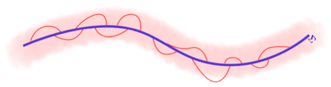 Figure 1
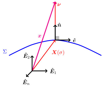 Figure 2
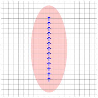 Figure 3
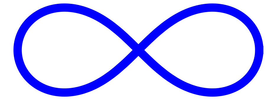 Figure 4
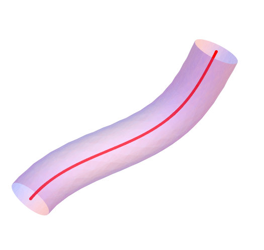 Figure 5
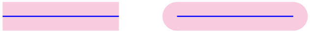 Figure 6
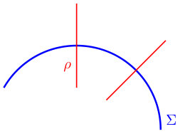 Figure 7
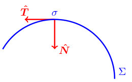 Figure 8
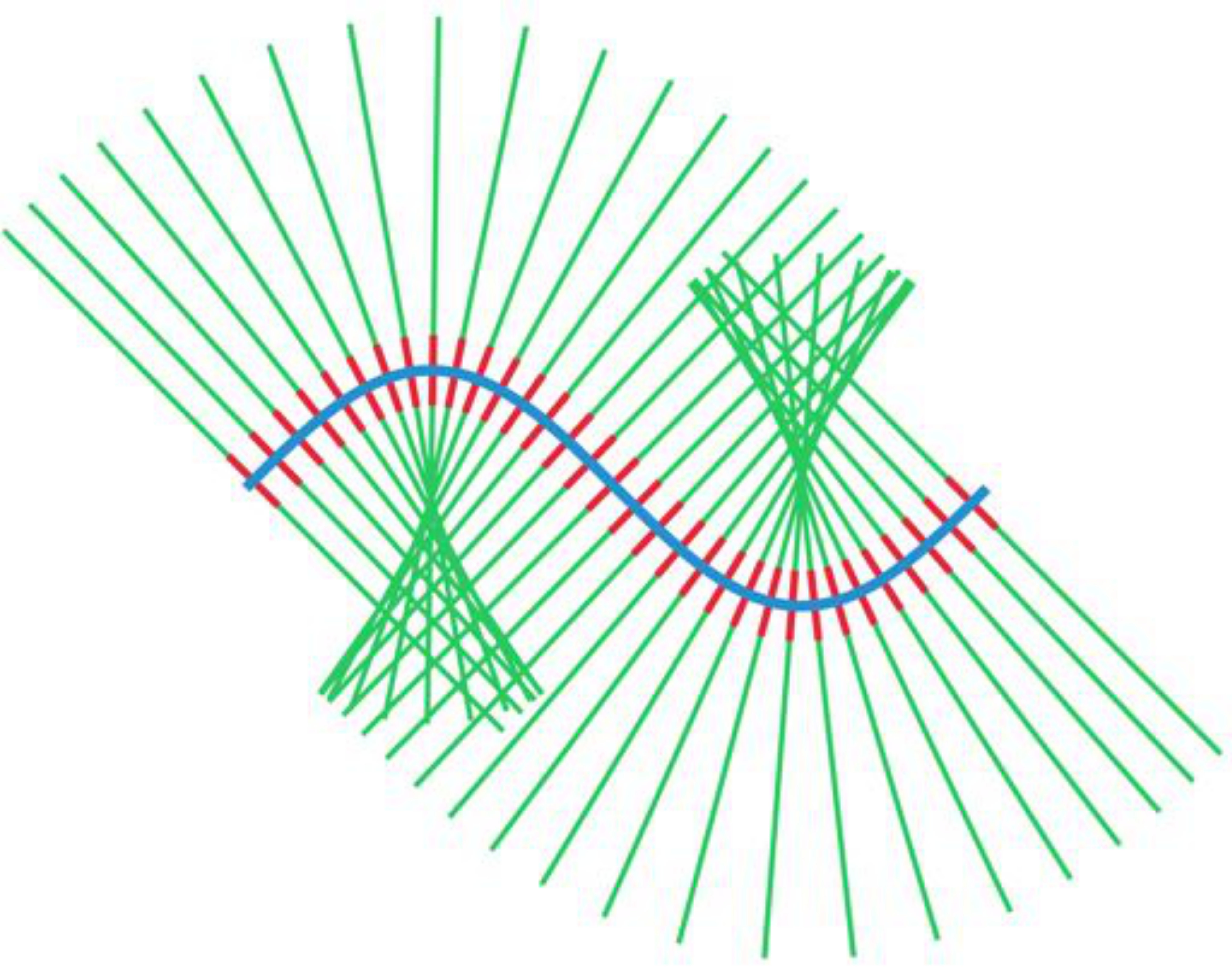 Figure 9
Peer Reviews
No public reviews on file for this paper yet. If you reviewed it on a platform where reviews are public (OpenReview, ICLR, NeurIPS, ICML), you can paste yours below so the community can read it here.
Videos
No videos yet. Explain this paper in a talk, walkthrough, or lecture? Add one.
Taxonomy
TopicsBlack Holes and Theoretical Physics · Cosmology and Gravitation Theories · Noncommutative and Quantum Gravity Theories
††institutetext: Department of Physics, University of Miami,
1320 Campo Sano Ave, Coral Gables, FL 33146 USA
Emergent Gravity and Weyl’s Volume Formula
Orlando Alvarez111This work was supported in part by the National Science Foundation under Grant PHY-1212337.
Abstract
In physical theories where the energy (action) is localized near a submanifold of Euclidean (Minkowski) space, there is a universal expression for the energy (or the action). We derive a multipole expansion for the energy that has a finite number of terms, and depends on intrinsic geometric invariants of the submanifold and extrinsic invariants of the embedding of the submanifold. This universal expression is a generalization of an exact formula of Hermann Weyl for the volume of a tube. We describe when our result is applicable, when our generalization gives an exact result, and when there are corrections (often exponentially small) to our formula. In special situations, dictated by spherical symmetry, the expression is a generalized Lovelock lagrangian for gravity, a class of theories that are interesting because they have no negative metric states. We discuss whether these results represent a true theory of emergent gravity by discussing simple models where a higher dimensional quantum field theory without a fundamental graviton leads to a gravity-like theory on a submanifold where all or some of the dynamical degrees of freedom are fluctuations of the metric on the submanifold.
1 Introduction
We consider physical systems where there is a localization of energy (or action) near a submanifold of Euclidean space (or Minkowski space ). What we argue in this article is that there is a universal expression for the energy (or the action), and we derive a multipole expansion for the energy that has a finite number of terms, and depends on intrinsic geometric invariants of the submanifold and extrinsic invariants of the embedding of the submanifold. We briefly discuss two potential examples.
First, consider a -dimensional D-brane Dai:1989ua whose time evolution is a dimensional submanifold222We write when we want to be explicit about . of -dimensional Minkowski space . Open strings of length , where is the Regge slope, terminate on a as in Figure 1. The open strings arise due to quantum fluctuations and this mechanism leads to an effective action density localized within a distance of near the submanifold . In a string theory, there are closed strings propagating in the bulk, i.e., the string theory has a bulk graviton. Theories of gravity of this type in a Kaluza-Klein compactification scenario were discussed in Antoniadis:1998ig .
A second example is the effective action for a topological defect Forster:1974ga ; Maeda:1987pd ; Gregory:1988qv . For concreteness consider the Nielsen-Olesen vortex in the Higgs model in . The surface corresponds to the -dimensional timelike submanifold that is the locus of where is the complex scalar field. The scalar field and the gauge field decay exponentially as you move away from therefore the action density of the theory also decays exponentially as you move orthogonally to .
The use of geometric concepts in computing the energy of a physical system has a long history in physics. For example, the very successful phenomenological liquid drop model in nuclear physics uses the short range nature of the nuclear force and the incompressibility of nucleons to argue that the binding energy of a nucleus with atomic number goes like . The first term is a volume energy term and the second term is a surface area term reflecting that the nucleons on the boundary have less neighbors for interaction.
In this article we derive a general expansion for models with localized energy near a submanifold in terms of the curvature invariants of the submanifold in question. The motivation comes from an formula due to Hermann Weyl for the volume of a tube Weyl:tubes . In the simplest models we will show that the dynamics of the theory is determined by an effective action with a finite number of terms with universal form:
[TABLE]
where is the metric on , is the Riemannian curvature tensor of that metric, and , and are effective fields on . In the simplest models for topological defects, the values of the fields are constants. In D-brane models, the field is the Dirac-Born-Infeld (DBI) Lagrangian, see Section 5.3.
The terms that appear to all orders in (1.1) are the “dimensional continuations” of the Euler densities known as the Lipschitz-Killing curvatures333Nineteenth Century mathematicians, R. Lipschitz and W. Killing were interested in invariant theory and in geometry. They wrote down these curvature expressions as geometrical invariants of a manifold without any inkling of the relationship to the topological invariants discovered by S.S. Chern much later.. From the physics viewpoint this is astonishing. Gravitational theories defined by Lagrangians containing those terms were discussed by Lovelock Lovelock:1971yv ; Lovelock:1972vz in the early 1970s who was interested constructing generalizations of the Einstein tensor. He required his tensors to be symmetric, rank two, divergence-free and to contain at most the first two derivatives of the metric. The appearance of Lovelock Lagrangians in string theory was first observed by Zwiebach Zwiebach:1985uq who noted that compatibility of a ghost free theory with the presence of curvature squared terms in the gravitational Lagrangian required a special combination that reduced to the Euler density in four dimensions. By studying the -graviton on shell vertex in string theory he verified that this curvature squared combination appears. Zumino Zumino:1985dp generalized Zwiebach’s results and showed that gravitational theories containing higher powers of the curvature given by a Lagrangian where the additional terms were “dimensional continuations” of Euler densities in the appropriate dimensionality, i.e., Lovelock type Lagrangians, were ghost free. A Lovelock gravitational action for a spacetime is constructed by taking linear combinations of specific curvature invariants:
[TABLE]
where is a coupling constant, is the volume element on , and the curvature terms are defined by (5.3). The contribution to the equations of motion from each action is a symmetric divergenceless second rank tensor that contains at most second derivatives of the metric Lovelock:1971yv ; Zumino:1985dp . These Lovelock Lagrangian densities arise in the context of this article because of a formula Weyl:tubes due to Hermann Weyl for the volume of a tube that we describe beginning in Section 2. What we derive here is a generalization of Weyl’s formula.
We mostly work in Euclidean signature and use the language of statistical mechanics or of Euclidean quantum field theory. We are interested in the isometric embedding of a -dimensional submanifold of Euclidean space . If the embedding444We use a hooked arrow to denote an embedding. is described by a map with then the metric induced from the embedding is
[TABLE]
and the induced Euclidean volume is
[TABLE]
The volume is invariant under the action of the Euclidean group on the embedding map and under the action of , the group of diffeomorphisms of connected to the identity. Note that the induced metric can be determined intrinsically via measurements performed on the surface.
We point out some related research that is not the main focus of this work. In our work we start with a higher dimensional theory without gravity and we obtain a gravity-like theory on a submanifold. This is dual to the work of Maldacena Maldacena:1997re ; Aharony:1999ti where in the bulk he begins with a theory of gravity and on the conformal boundary he has a Yang-Mills theory. We are not aware of correlation function relations as in the Maldacena duality.
In some sense, the most elegant theories of emergent gravity are topological such as the A and B topological theories Witten:1988xj ; Witten:1988ze ; Bershadsky:1993cx . We do not see a direct connection of our work to these since we begin in a metric space or .
Our work is also related to theories for emergent gravity or gravity on submanifolds. There are many scenarios and our research touches three major areas. There is a lot of work on models to explain the relative weakness of the gravitational force in four dimensions starting with a theory of gravity in higher dimensions. They are the Kaluza-Klein type models of Antoniadis, Arkani-Hamed, Dimopoulos and Dvali ArkaniHamed:1998nn ; ArkaniHamed:1998rs ; Antoniadis:1998ig (AADV) and their variants where a TeV scale higher dimensional gravity with a compactification scale large compared to the Planck length leads to a four dimensional gravity theory with the experimental value for the Planck mass . There are also the models motivated by the work of Randall and Sundrum Randall:1999vf ; Randall:1999ee . Here the universe is a slice of with two boundary pieces of which one is the physical -brane we inhabit. The radius of curvature of the and width of the slice are Planck length order of magnitude. Randall and Sundrum use the exponential change in the metric as you move from the hidden slice to the visible slice to generate an exponential hierarchy where the physical field theoretic parameters on the visible slice are TeV scale. An extension of the work presented here to the case of embedding in constant curvature spaces and the Randall-Sundrum scenario appears in a companion article Alv:2016b . There are also the models of emergent gravity motivated by the work of Dvali, Gabadadze and Porrati Dvali:2000hr where gravity on an infinite five dimensional spacetime reproduces the correct crossover to 4 dimensional behavior on a 4 dimensional submanifold. The focus of this paper is theories that do not contain gravity in the bulk but lead to a gravity-like theory on a submanifold. A phenomenon like this happens in theories of defects but we explain carefully in Sections 7 and 8 that these do not necessarily lead to a theory of emergent gravity.
2 The classical physics of tubes
We first define a tube and subsequently discuss the physics of tubes. An Euclidean tube, in the sense of Hermann Weyl’s classic paper Weyl:tubes , is a way of thickening a submanifold of Euclidean space . For example, the thickening of a point will be a small ball. An obvious thickening of a line in is a solid cylinder of small radius. A natural thickening of the -dimensional submanifold in is the -dimensional tube, , of radius constructed from by thickening the submanifold by moving orthogonally to the submanifold a distance , see Figure 2. The technical mathematical definition Gray:tubes is given below.
Definition 2.1** (Weyl Tube).**
Let be an embedded compact submanifold without boundary, i.e. a closed submanifold. The tube of radius about is a subset of with the following characterization: is in the tube if there exists a straight segment from to that intersects perpendicularly and the length of the segment is less than or equal to , see Figure 2. The tube is a fiber bundle over with fiber , the -dimensional ball (the solid -sphere).
Remark 2.2*.*
In this article we relax the requirements on the definition of a tube by allowing submanifolds that are not compact but have no boundary such as a -dimensional vector subspace of .
Clearly the tube changes as we vary the extrinsic geometry of while keeping the intrinsic geometry fixed555A cylinder and a -plane in have the same local flat intrinsic geometry but the extrinsic geometries are very different. Throughout this article we always implicitly assume that the radius of the tube has to be small enough so that there are no (local) self intersections. For example, the extrinsic radii of curvature of should be large compared to , see Figure 3. Note, the local restrictions on the radius of the tube and the radii of curvature are not sufficient to guarantee that globally we will not have self intersections, see Figure 4. If has a boundary then there are technicalities and we do not study this case here, see Figure 5 and Reference Gray:tubes . In this article we only consider “nice” tubes and we avoid all subtleties and technicalities.
We first discuss an artificial and mostly academic physical model: the classical dynamics of a tube. When we embed a -submanifold, the standard action is proportional to the -volume of the submanifold. A tube is an -dimensional submanifold, hence the classical action should be:
[TABLE]
where the tension has dimension . There are no bulk curvature terms to be included in the action because the bulk metric is the flat Euclidean metric. In principle there could be geometric terms in the action associated with the dimensional boundary of the tube but we ignore these.
The dynamics of an -submanifold governed by the volume action is very general. Imagine an -ball with boundary waves or the -ball deforming itself to a cylindrical configuration; there are endless possibilities. The dynamics of a tube are much more restrictive. There is an instructive classical mechanical analogy. The motion of interacting particles in is intractable but the motion of a rigid body made up of particles has a six dimensional configuration space: three translational degrees of freedom and three rotational degrees of freedom. Additionally, the kinetic part of the action of a rigid body only depends on a small number of parameters: the total mass and the moment of inertia tensor of the body. Two body potentials that are translationally and rotationally invariant will only contribute a constant to the action of a rigid body. An external constant gravitational field will give an effective potential energy that depends on the position of the center of mass. These simplifications lead to an action for a rigid body with tractable equations of motion.
The restriction to the study of the classical motion of a tube and not to a general -submanifold greatly constrains the dynamics because the tube is uniquely determined by the underlying base manifold and the radius . What is surprising is that the action (2.1) may be expressed solely in terms of the intrinsic geometry of because of a celebrated formula (5.11) for the -volume of a tube due to Hermann Weyl Weyl:tubes . This formula has exactly terms and the first three are:
[TABLE]
In the above , and is the -volume of the unit -ball (see eq. (B.2)), is the Riemann curvature tensor of the induced metric on , and is the intrinsic volume element of the induced metric on . The dynamics of the -dimensional tube is determined by an action for the motion of the -dimensional base of the tube. The terms that appear to all orders in in Weyl’s tube volume formula are the “dimensional continuations” of the Euler densities. We refer the reader back to the Introduction (Section 1) where the significance of such terms is discussed.
Firstly, we remark on a couple of surprising results that follow from the Weyl volume formula. If we thicken a closed curve then the volume of the tube will be where is the length of the curve. This result is what you would expect for a right circular cylinder and is independent of the shape of the embedded curve. In the case of a closed surface , we have the exact result . Notice that the first summand is the naive volume of a slab of thickness centered about .
Secondly, a remarkable property of Weyl’s formula is that the volume of the tube depends only on the intrinsic geometry of , i.e., the induced metric and not the extrinsic curvatures. The only features of the embedding that appear in the formula are the dimensionality of the embedding space (via ) and the radius of the tube . The extrinsic curvatures (second fundamental forms) that characterize the embedding of do not appear.
If we combine the Weyl volume formula with (2.1) then we see that the classical action of tubes is governed by the same action as generalized Lovelock theories of gravitation in -dimensions. The first term is a -brane tension for the -brane, , and the second term in the expansion is the Einstein-Hilbert action with -dimensional gravitational constant . Note that the conventionally defined cosmological constant is is independent of the tube tension . What we have here is a gravity-like action that emerges from embedding dynamical tubes in Euclidean space. There may be no fundamental graviton in but it is possible that a graviton on emerges because of the fluctuations of the embedding. This is in the same sense that phonons emerge from lattice vibrations. Whether or not we have an emergent graviton is discussed in Section 7 and is related to the mathematics of isometrically embedding submanifolds in Euclidean space. In the case that we have a de facto graviton, the classical physics of the dimensional tube is the same as -dimensional Lovelock gravity for the spacetime .
3 Energy tubes
Tubes in the sense used by Weyl are mathematically interesting but it is difficult to envision a physical phenomenon that would lead to their existence. In this section we consider a generalization of Weyl tubes that we will call energy tubes. In Minkowski space these should more properly be called action tubes. We can construct physical systems that lead to energy tubes and we describe several possibilities in this section. An energy (action) tube is a localization of energy (action) near a submanifold.
We motivate the basic idea of an energy tube with a phenomenological discussion within the -dimensional Ising model. The Ising Hamiltonian is where is the spin at lattice point , denotes a nearest neighbor pair, and is the temperature of the heat bath. Assume we are in the disordered phase, , with finite correlation length . Suitably averaged, the energy density will be constant throughout the plane.
We now modify the system by introducing a finite “wall” where the spins are all fixed to point up as in Figure 6. At distances much larger that the correlation length , the thermodynamic system will be unaware of the wall and the energy density will be just as in the Ising model without the wall. Near the wall, i.e., within several correlation lengths of the wall, the distribution function for the fluctuating spins will be affected by the “wall boundary conditions” and we expect a different energy density. If is the difference between the energy densities in the two models then we expect most of the support of to be localized in a region similar to the shaded one in Figure 6. The function should decay exponentially to zero as you move away from the wall. The shaded region in Figure 6 is an energy tube that arises because of the boundary conditions on the wall. Other models of defects with non-zero correlation lengths will have the same property of energy localization near the defect.
A model for constructing energy tubes begins with a field theory on specified by fields . We introduce an embedded submanifold and the coupling of to the fields is by the imposition of special boundary conditions on the submanifold in analogy to the way a perfectly conducting plane interacts with an electrostatic field. Another method is -brane type couplings; the coupling of a -form to is of the form .
From the path integral viewpoint the partition function you are computing is
[TABLE]
where is the embedding, is the space of all field configurations compatible with the boundary conditions imposed by the embedding of , and is the action for the fields. The integral over depends on via the map because the coupling of to the fields is through the boundary conditions. The free energy due to the fields is
[TABLE]
Let be the free energy due to in the absence of , and let be the relative free energy. The full partition function (3.1) becomes
[TABLE]
The problem is computing . We will use some mean field theory arguments to propose a form for . A précis of the subsequent paragraphs is that if all fields are massive then the presence of leads to a relative free energy density function666We use the letter as a generic energy density whether it be regular energy or free energy. that should decay exponentially as you move away from . The energy tube is located where is “large”. An energy tube does not have a fixed radius as a Weyl tube; the energy density drops off as you move away from . We assume a mean field type form for the energy given by an energy density :
[TABLE]
We emphasize in the formula above that the free energy density depends on the embedding . A generalization of Weyl’s formula for the volume of a tube will be used to evaluate (3.3) and show that it has a universal form depending of a finite number of terms.
Another well known example of boundary conditions changing the energy density is the Casimir effect. For the discussion here we switch to quantum field theory language in Minkowski space . The field theory is free photons in the presence of two perfectly conducting planes. The electromagnetic field has to satisfy some special boundary conditions. The energy of the system is determined by the zero point fluctuations of the electromagnetic field. The normal modes for the electromagnetic field in the system with plates are different from the ones without plates resulting an attractive force between the plates. This is a system with massless particles and therefore the discussions given in this article are not valid.
4 Weyl’s volume element formula
Even though Weyl’s paper is about the volume of tubes what he actually derives is a formula expressing the Euclidean volume element in terms of the volume element on the submanifold , and “polar coordinates orthogonal to ”. We provide a more modern derivation of Weyl’s result Weyl:tubes below. Weyl’s expression for the volume element is what allows us to consider a multipole expansion for the energy.
Let be a standard orthonormal cartesian basis for . If then we assign coordinates to that point by . Let the map be an embedding of the image in Euclidean space. Then for each we have an orthogonal direct sum decomposition of the tangent bundle where is the normal bundle at . In a small tubular neighborhood of , we can describe a point uniquely by
[TABLE]
where , see Figure 7. Locally choose an orthonormal frame for and an orthonormal frame for . Such a frame is called a Darboux frame. Note that . Let be the inclusion map and let be the bundle of orthonormal frames of . The set of all Darboux frames of is a sub-bundle of the pullback bundle with structure group , where . Let be local coordinates on and let , then are local coordinates for the tubular neighborhood. Our index convention is that latin indices from the beginning of the alphabet go from to , latin indices from the middle of the alphabet go from to , and greek indices go from to . Next, we take the differential of (4.1) and follow standard moving frame techniques developed by E. Cartan Cartan:riemann (see BCG3 for the general theory) to study submanifolds of Euclidean space. First, note that where the are -forms on because , and the “displacement of ”, , is tangential to the surface. We observe that orthonormality requires
[TABLE]
Since and are defined only on , it follows that and are -forms on . The connection -form on is . The connection -form on the normal bundle is , and are the extrinsic curvatures (second fundamental forms). Next we note777We are in so the covariant exterior differential is the ordinary one. , and putting all this together we see that
[TABLE]
where is the covariant differential on the normal bundle. Using the fact that is an orthonormal frame and that , we see that an orthonormal coframe at is given by (\hat{\theta}^{a},D\nu^{i})=\bigl{(}(\delta_{ab}+\nu^{i}K_{abi})\theta^{b},D\nu^{i}\bigr{)}. Therefore, the Euclidean metric is given by
[TABLE]
where
[TABLE]
We mention that the results above are also valid in Minkowski space if the normal bundle has Euclidean signature, and the tangent bundle has Lorentzian signature. Observe that in Minkowski space has signature and therefore in eq. (4.5) is implicitly interpreted to be where is the Minkowski metric on .
The volume element is easily computed in the orthonormal coframe
[TABLE]
The maximum number of powers of is already present in the expression above, hence we can replace by and obtain Weyl’s formula for the Euclidean volume element in a tubular neighborhood of :
[TABLE]
where is the volume element on .
We mention that the Weyl volume element formula (4.6) is also valid in Minkowski space as long as the submanifold is timelike. Note that the normal tangent bundle has Euclidean signature and our derivations are valid. The volume element is now the Lorentzian volume element on .
Taking a Minkowski space field theory viewpoint, we point out that enters into the Lagrangian for scalar fields and enters into the Lagrangian for vector fields, and these can be computed in the Darboux frame using the formula (4.4) for the metric. In computing the action of a field theory we expect to find terms of the type
[TABLE]
The main result of this paper is a general formula for the potential energy like term (4.7a) which involves a finite number of monopole moments that is a generalization of Weyl’s volume formula. The kinetic energy like terms, (4.7b) and (4.7c), lead to an infinite power series in . We have not found a re-expression of those formulas that leads to anything resembling the simplicity of Weyl’s volume formula. As a field theory on , we note that time derivatives will only appear in (4.7b) and (4.7c). For the rest of this paper we concentrate on evaluating (4.7a).
5 The energy contained in an energy tube
Let be the energy density at , then the energy in a small volume is given by . Because we are interested in the energy density near , it is convenient to use Weyl’s volume element (4.6) formula to express the total energy as
[TABLE]
In general, the normal bundle integral cannot be performed. Here we show that if decays rapidly enough away from then it has a multipole expansion, and the normal bundle integral can be simplified and expressed in terms of a finite number of radial moments associated with the energy density. The derivation of the general formula is quite technical and we defer it for the moment; instead, we first discuss what the answer looks like in the important special case of spherical symmetry.
5.1 The spherically symmetric case
There are interesting examples where the energy density function is spherically symmetric in the normal bundle, namely, . We refer to this as a monopole energy density. The energy is given by
[TABLE]
First we define some curvature invariants associated with the intrinsic geometry of . The curvature -form is , the Hodge dual of is , and other notations are explained in Appendix A. Let
[TABLE]
The first three are:
[TABLE]
The defined here are the same as the in Gray (Gray:tubes, , p. 56). These are the curvature combinations identified by Lovelock that lead to generalizations of the Einstein tensor.
If is even then the differential form of maximal degree is
[TABLE]
where is the Pfaffian of the “antisymmetric matrix valued -form” . The Euler characteristic of is by the general Gauss-Bonnet Theorem of Chern.
Next we define the “normal radial moments” of the monopole energy density by
[TABLE]
where is the -volume of , see Appendix B. The energy of the tube is given by
[TABLE]
where are constants specified by (B.6). Note that the energy only depends on the intrinsic geometry of . The derivation of this formula is presented in detail in Section 6.2. Is equation (5.6) actually an equality or is it an approximation? We defer this question to a post-derivation discussion in Section 6.2.
The discussion of Section 2 can now be applied to the monopole contribution to the energy (5.6). The effect of the bulk QFT that lives on is to produce effective scalar fields that couple linearly to Lovelock type curvature terms. Note that these effective fields live on and in the very small curvature situation we can approximate them as being constants. To “leading order” we would replace the fields by constants . The net effect of the bulk QFT to leading order is to induce an effective action for the surface that is a Lovelock type gravitational action.
The symmetric Lovelock tensors are the generalizations of the Einstein tensor proposed by Lovelock. The -th one is defined by the variational derivative of the parent Lovelock action , see (1.2) or (5.6),
[TABLE]
Since each action is diffeomorphism invariant, the corresponding Lovelock tensor is automatically conserved . For example, the Lovelock tensor is precisely the Einstein tensor . A straightforward computation gives
[TABLE]
If is even then because the multi-index -tensor is identically zero since it involves total antisymmetrizations. The vanishing of is a consequence of the topological nature of .
5.2 The volume of a tube
An example of the spherically symmetric case is an energy tube with constant energy density out to a radius and vanishing beyond:
[TABLE]
The moments are given by
[TABLE]
In this case the energy will be and we obtain Weyl’s formula for the volume of a tube:
[TABLE]
Note that
[TABLE]
Using (B.2) and putting it all together, we have Weyl’s formula for the volume of a tube:
[TABLE]
The defined here are the same as the in Gray (Gray:tubes, , p. 56). The equation above may also be written as
[TABLE]
5.3 Dirac-Born-Infeld action
The effective action for D-branes is the Dirac-Born-Infeld action, for a review see Johnson:D-branes . The DBI action in a coordinate basis is usually written as where is an antisymmetric -tensor. If we go to an orthonormal frame we see that the DBI action is
[TABLE]
where the matrix elements of are the components of the antisymmetric -form in the orthonormal frame. This corresponds to a monopole moment of the form .
6 The multipole expansion for the energy
6.1 Spherical harmonics
In general, the energy density will not be spherically symmetric, see Figure 8. To proceed with the evaluation of (5.1) we use a multipole expansion. Let and write where .
Group representation theory tells us that the real valued functions on decompose into an orthogonal direct sum of real finite dimensional irreducible representation spaces of , i.e., is an irreducible real -module. The standard expansion for in terms of spherical harmonics is given by
[TABLE]
where is a real orthogonal basis of spherical harmonics for the sphere with normalization
[TABLE]
The index refers to the “spin ” representation of ; we will make this precise soon. A result we wish to establish in this section is that the total energy (5.1) only depends on the first multipole moments of (6.1), i.e., . To prove this observation and to discuss the evaluation of the integral (5.1), it is better to use cartesian spherical harmonics that we will describe shortly. The proof requires understanding the relationship between polynomials in the variables and the spherical harmonics.
Think of the cartesian coordinates as a basis for the real vector space888A coordinate function on vector space is a linear functional and therefore the coordinate functions are basis for the dual vector space of but because we have a metric we implicitly identify with its dual space . . In other words, we write as a linear functional . acts on irreducibly. The set of homogenous polynomials of degree are isomorphic to the -fold symmetric tensor product . The space is invariant under the action of but the action is not irreducible because of the existence of the trace operation. The monomials span but tracing on the last two indices leads to monomials and the span of these homogeneous polynomials of degree (isomorphic to ) is an invariant subspace of . Our irreducible representation space is isomorphic to the vector space of rank symmetric traceless tensors. A spanning set related to the spherical harmonics on the sphere may be constructed from the homogeneous degree polynomials in the following way. We restrict the homogeneous polynomials to the unit sphere by imposing the condition . Restriction to the sphere turns a homogeneous degree polynomial into an inhomogeneous polynomial with respect to degree because every occurrence of is replaced by . We will refer to the spanning set as the faux cartesian spherical harmonics on because they are not a basis but an over complete spanning set. Our notation for the faux spherical harmonics is . The first few faux cartesian spherical harmonics are
[TABLE]
For , the faux cartesian spherical harmonics are uniquely specified by
is totally symmetric under any permutation of . 2. 2.
is traceless with respect to contraction on any pair of indices. Because the faux harmonic is totally symmetric in the lower indices, this reduces to . 3. 3.
The parity of is . 4. 4.
is an inhomogeneous polynomial of degree in the with normalization determined by
[TABLE]
Let be the defining representation space of and let denote the -th symmetric tensor product, . For fixed , the span of is a real irreducible -module (an irreducible representation in a real vector space) that we denote by . The representation space is isomorphic to the space of symmetric traceless tensors of rank . The are in general not linearly independent. For example, if then the tracelessness condition tells us that . The spherical harmonics are a basis for but the faux harmonics are an over complete spanning set if . For and we can choose and .
Next we define cartesian multipole moments by writing
[TABLE]
In the above we require to be totally symmetric and traceless in the indices . The symmetric traceless tensor is well defined.
is a reducible representation and we have a direct sum decomposition into irreducible representations (FultonHarris, , Exercise 19.21)
[TABLE]
You can verify that , , and
[TABLE]
To proceed with the evaluation of the energy we have to make some assumptions about . Not all these assumptions are required by the mathematics, but they are motivated by physics considerations. We require to decay rapidly enough as . In many examples you have exponential decay. We are interested in weak gravity and thus we expect the curvature of to be small. To first approximation and in this case we expect the energy density to be translationally invariant with respect to and probably spherically symmetric in the normal bundle direction. As the surface starts to curve we expect that the higher multipole moments are built up. Schematically we assume a hierarchy with where we use the symbol to indicate a vague hierarchical structure in magnitude. We also assume the are slowly varying functions of .
To evaluate the energy we focus on the parenthetical expression in (5.1), apply (A.7) and obtain
[TABLE]
In the expression above we have to perform the angular integral
[TABLE]
To understand the result of this integration we use the decomposition (6.5) and expand using our basis of spherical harmonics:
[TABLE]
for some constant coefficients . Note that in the sum above you only get spherical harmonics with parity . Inserting this expansion into the angular integration (6.8) we see that result of the integration can only involve the multipoles . Next we observe that in the basic integral (6.7), the sum over goes from [math] to and therefore the energy of the energy tube will only depend on the first multipole moments . This result is surprising. Higher multipole moments for the energy density correspond to finer grained angular resolution in the normal tangent space . The total energy of an energy tube is insensitive to variations in the energy density on angular scales smaller than roughly radians.
6.2 The monopole contribution
To evaluate the monopole contribution to the energy we return to equation (6.7) and replace by and obtain
[TABLE]
To perform the integral we used the averaging results derived in Appendix B. Next we use the Gauss equation
[TABLE]
to convert extrinsic curvature terms into intrinsic curvature terms:
[TABLE]
Rewrite the above using the curvature -form and identity (A.4) to obtain
[TABLE]
where
[TABLE]
Next we define the “normal radial moments” of the monopole moment of the energy density by
[TABLE]
Collating everything we have the monopole contribution to the energy
[TABLE]
We now address the question of whether the finite series in eq. (6.13) is exact or an approximation. Assume the integrable function is compactly supported in a nice tube999The radius of the tube is small enough so that there are are no self-intersections. . In this case, equation (6.13) is exact. This is quite a surprising result, and the main mathematical result of this paper along with its generalization (6.24) to non spherically symmetric functions. It states that the integral of a spherically symmetric compactly supported function may be described in terms of a much smaller set of data: functions defined on . This universal form tells us that only some general features of the energy density function survive after integration. Namely, a finite number of radial moments. The prime example of this integration result is the Weyl volume formula (5.12). If the radius is too large and there are self intersections. then formula (6.13) will not be valid. This can be seen by looking at Figure 3 and observing that certain volumes will be over counted in attempting to perform the integration by first integrating over the normal bundle. This result for compactly supported energyt densities motivates why there is a universality in the type of effective field theories that are induced on from the ambient bulk physics.
In most physical applications, the energy density does not have compact support. In quantum field theories with massive excitations you expect some type of exponential decay of the energy density with a correlation length as you move away from :
[TABLE]
where in many models. If is characteristic of the distance at which you find the nearest self intersection of the tube, and if you assume that , then you expect the there will be exponentially small corrections to (6.13) of order , note that :
[TABLE]
Is there an expansion parameter for the individual summands in (6.13)? The answer to this question was essentially given in the caption of Figure 3. In the context of our exponentially decaying energy density we would like for . We naively estimate the ratio of the summands in the expansion. First we assume that the couplings are independent of such as in the case of a spherically symmetric defect, see Section 8.1. If we think of as an effective dimensionless energy or effective action entering a Boltzmann factor then the dimensions of are . For a static defect, the energy density is translationally invariant along the defect and we expect from dimensional analysis that , where is some -dimensional energy scale, and the -dimensional energy density will be identified with the -brane tension. For example, could be a correlation length in some quantum field theory that interacts with the submanifold . Note the dimensional units of are . From eq. (6.12) we see that . Since is the coupling of the -volume contribution, it is the -brane tension and we immediately have its identification with . Note that the ratio of couplings . The -dimensional reciprocal Newtonian gravitational constant . There is a dependence on through the coefficients that we have not taken into account in our very rough estimates. The Gauss equation tells us that, roughly, . An estimate of the -th summand in (6.13) is given by
[TABLE]
Thus expansion parameter in this spherically symmetric energy density model is .
6.3 The dipole contribution
To evaluate the dipole moment contribution to the energy we begin with equation (6.7), replace by , and obtain
[TABLE]
This may be expressed in terms of differential forms by introducing the extrinsic curvature -forms101010The Riemannian connection in a Darboux frame adapted to is the same as .
[TABLE]
The complicated expression above becomes
[TABLE]
Mimicking (6.12) we define the normal radial moments of the dipole moment of the energy density by
[TABLE]
Putting it all together we see that the dipole contribution to the energy is given by
[TABLE]
6.4 The general multipole contribution
The contribution to the energy from the cartesian -pole is given by (see (6.7))
[TABLE]
The spherical integral vanishes unless is an even number. The expression above may be rewritten as
[TABLE]
where the summation set will be specified shortly. is a sum of summands constructed from Kronecker -symbols, see eq. (B.4). A summand that contains contributes zero to the sum because is traceless. Hence each “” index must be contracted with an “” index to obtain a non-zero contribution. Thus we conclude that non-vanishing terms must have where . Inserting this information into the displayed equation above yields
[TABLE]
Remember that the total number of indices in is . The number of summands in that give a non-vanishing contribution is
[TABLE]
Define the radial moments of the -pole by
[TABLE]
Note that the moments are a section of the vector bundle (over ) which is the symmetric traceless subspace of the -th tensor product of .
Inserting the radial moments definitions (6.22) into (6.19) and using the Gauss equation to rewrite some of the factors as the intrinsic curvature leads to
[TABLE]
The last expression above may be rewritten using differential forms and we obtain the following expression for the contribution of the -pole to the energy
[TABLE]
As a check you can verify that the expression above reduces to (6.13) in the monopole case and (6.18) in the dipole case. Notice that if is even then the moments that occur are ; and if is odd you get .
The Gauss equation (6.9) may be written as and the -curvature -form of the normal bundle is (the dual Gauss equation). Since the cartesian multipole moments are traceless in the indices, we see that the terms in (6.23) cannot be transformed into terms involving the intrinsic curvature of the surface. Note that the curvature of the normal bundle does not appear. For completeness, we note the Codazzi-Mainardi equation .
Now we can write down a multipole expansion formula for the total energy of an energy tube:
[TABLE]
In the above, the superscript ST means orthogonal projection onto the symmetric traceless part on the -indices. The total number of moments is where is a function of . It is quite interesting that integral (5.1) is given by the finite number of terms in (6.24).
We now repeat an earlier discussion in the spherically symmetric case. Is the the finite series in eq. (6.24) exact or an approximation? Assume the integrable function is compactly supported in a nice tube111111The radius of the tube is small enough so that there are are no self-intersections. . In this case, equation (6.24) is exactly the value of the energy density integral. If the radius is too large and there are self intersections then formula (6.24) will not be valid. If then energy density decays exponentially then we expect exponentially small corrections to (6.24) as in the spherically symmetric case.
If gets a vacuum expectation value (VEV), the structure group of the normal bundle is reduced to a subgroup that leaves the VEV invariant. In this way you could have some type of Nambu-Goldstone or Higgs mechanism on .
The expansion parameter for (6.24) is due to the presence of the extrinsic curvature terms rather than in the spherically symmetric case (6.13).
7 Embeddings and emergent theories of gravity
We begin with a differentiable -manifold and we are interested in embedding121212We ignore the technical differences between an embedding and an immersion. in Euclidean -space . The reason for embedding is that we will assume that there is a quantum field theory (QFT) on and we are interested in discovering the effect of the interaction of the QFT with the embedded submanifold. The role of the QFT is to provide a localized energy density near . In this section we discuss the dynamical equations that arise when we vary the embedding. In Section 8 we address additional dynamical equations that arise due to variations in the energy density near .
Before exploring the consequences of the embedding we digress and explain what will not be considered in this paper. The manifold could be endowed with intrinsic geometrical structures that are not related to the embedding. For example, assume has a Riemannian metric . We expect the action that determines the dynamics of to be of the form if is a dynamical field. In such a situation we see that we will have -dimensional gravitation on a priori of the embedding. We will not discuss this case at all, see for example Dvali:2000hr . The problem we address is the one where is a plain differentiable manifold with no intrinsic structures and its geometry is induced by an embedding in an Euclidean space with a bulk QFT. We address the question whether potentially an effective theory of -dimensional gravity on emerges because of the embedding. There is no fundamental graviton in the Euclidean space but the dynamics of the submanifold can effectively be described by a gravity-like theory that only lives on the submanifold. In this section we discuss the meaning of gravity-like.
It is worthwhile to be mathematically precise to better understand the goals of this section. An embedding is given by a map . We denote the embedded submanifold by . Note that and thus we have an inclusion map . If is the Euclidean metric on then the induced metric on given by the pullback . This induced metric on may be viewed as a metric on by pulling back again: , see equation (1.3).
If is -manifold with an intrinsic metric then is an isometric embedding if . To truly have a theory of gravity, it is necessary that you obtain all admissible intrinsic metrics on via embeddings. For this to occur, various general theorems impose restrictions on , the dimensionality of the embedding space.
The Nash embedding theorem and its refinements, see Greene:isometric ; Clarke:embedding ; Berger:PNAS ; Bryant-Griffiths-Yang:isometric and references therein, provide bounds that state that a smooth () isometric embedding of a riemannian manifold in euclidean space exists locally if and globally if . For real analytic () data, the isometric embedding theorem of Burstin-Cartan-Janet-Schläfly Berger:PNAS ; Berger:big states that a local real analytic embedding exists if . It is believed that the proven local bounds are not optimal and that the local threshold131313See the discussion in Terry Tao’s notes about P. Griffiths’ work and comments by D. Yang in http://terrytao.wordpress.com/2014/08/13/khot-osher-griffiths. S.T. Yau informs me that a motivation for the conjecture is that mathematicians have looked very hard but have not found a counterexample. is actually .
The theorems discussed in the previous paragraph apply to a generic manifold. For very special manifolds, the bounds are smaller. For example a dimensional vector space with the Euclidean metric can be globally isometrically embedded in any with . The unit sphere with the round metric can be globally isometrically embedded in any with .
Remark 7.1*.*
The dimension bound for a local analytic isometric embedding of a Lorentzian manifold in Minkowski space is also according to Eisenhart (Eisenhart:RG, , p. 188). If a -manifold has metric with signature where , and if you would like to locally analytically embed isometrically in with signature where , then you need , and and constrained by , and . Global embedding theorems for Lorentzian manifolds analogous to the Nash theorems are discussed in Greene Greene:isometric , and in Clarke Clarke:embedding .
The induced metric141414From now on we think of the embedding as being an isometric embedding and we identify the induced metric from the embedding with an intrinsic metric . is given by . If we vary the map then the change in the induced metric is
[TABLE]
where is the variation of the map, a -form on the space of maps . Next we express in terms of a deformation tangential to the surface and a deformation orthogonal to the surface151515See Section 4 for the notation. using an adapted Darboux frame
[TABLE]
where and are -forms161616The condition imposes some constrains on the differentials of the -forms and : and . on the space of maps . Inserting this decomposition into (7.1) we see that
[TABLE]
where . As expected, the tangential projection of the deformation is a vector field along the surface and thus the variation of the metric contains a part that is an infinitesimal diffeomorphism given by the Lie derivative . Equation (7.3) is the differential of the map given by (1.3). What are the conditions that the differential map (7.3) be surjective? On the left hand side of the equation, we have functions on ; the Lie derivative term on the right hand side involves functions on . For surjectiveness of the differential map, we require that the map given by have at least linear transformation rank171717The word rank is used in two different senses in this paper: firstly, in the linear algebraic sense of the rank of a linear transformation; secondly, in the sense of the rank of a vector bundle, i.e., the dimensionality of the fiber. . This means that, in the vector bundle sense, . For surjectiveness of the differential map, we need that the dimension of the embedding space satisfy . This agrees with the naive counting in PDE system (1.3) consisting of first order PDE for the embedding functions . To obtain an isometric embedding you need at least functions to naively avoid having an over determined system of PDE.
If you take a general Lovelock action (5.6) and you vary the embedding you will get
[TABLE]
In the above, are the conserved Lovelock tensors (5.8). The equation of motion that you get from the tangential variations is
[TABLE]
This equation is a reflection of the invariance of the action. In fact, since each summand in (5.6) is invariant, each identically. The equations of motion arising from varying the embedding in directions normal to the surface are
[TABLE]
There are two cases to consider.
First, assume that . Our previous discussion shows that we get all possible metric variations , and we can immediately use (7.4a), and conclude that the equations of motions are
[TABLE]
The equations of motion for the dynamics of are those of an euclidean Lovelock theory of gravity. Classically, this looks like an emergent theory of gravity where there is a graviton-like excitation on the surface. There are no negative metric graviton states. Note that these equations just involve intrinsic geometrical data on and are not aware of the embedding. We remind the reader that there may be additional equations that arise from the fields in the surrounding QFT and these are discussed in Section 8.
The next case is where . In this case you do not expect that all possible deformations of the surface lead to all allowed intrinsic metrics on the surface. Here you cannot use (7.4a) directly but must use (7.4b) that tells you which variations of the metric you obtain by varying the embedding. The equations of motions that follow are the tautological equations (7.5) and a subset of the Lovelock equations given by (7.6). You get a gravity-like theory but it is not gravity in the sense that the excitations are not gravitons as we explain below.
We study (7.6) the weak field linearized approximation. By the remarks in Zumino Zumino:1985dp , the only linearized term that is dynamical is contained in the ordinary Einstein tensor . If we write the weak field metric on the surface181818For the remaining part of this section we denote the metric on as . as , and if we define the auxiliary variables , then
[TABLE]
The linearized Einstein tensor is gauge invariant under the linearized gauge transformation , or . Next we use a gauge transformation and gauge fix in Lorenz gauge . This imposes conditions on the functions and leaves us with functions that encapsulate the Euclidean degrees of freedom. Imposing Lorenz gauge on (7.8) leads to
[TABLE]
where there are only independent functions . These manipulations only require properties of the linearized Einstein tensor.
If , then we are in situation (7.7), and the dynamics of are the dynamics of gravity governed by the wave equations (7.9).
If , the dynamics of are described by (7.6). As far as counting degrees of freedom, we can treat as constants and the linearized equation of motion in Lorenz gauge becomes
[TABLE]
Generically you expect the map191919The map is essentially the adjoint of the map previously discussed. to be surjective in the case with . This means that there is a non-trivial kernel with . Thus we have dynamical fields with that satisfy (7.10), and there are linear combinations of the metric fluctuations that vanish automatically and do not satisfy the Laplace equation. The metric perturbations in the kernel of are not dynamical. The number of degrees of freedom of this theory are less than the number of degrees of freedom in a gravitational theory. On the other hand, the degrees of freedom here, , are linear combinations of the metric fluctuations, and in this sense the theory is gravity-like. The properties of these gravity-like theories should be explored.
Remark 7.2*.*
Note that , and therefore we conjecture that the dynamical degrees of freedom beyond the weak field approximation in the case are the mean curvature vector density, .
Remark 7.3*.*
The counting of degrees of freedom is different between gauge theories in Minkowski space and in Euclidean space. In Minkowski space folklore “each diffeomorphism gauge transformation kills twice”. The reason is that once the Lorenz gauge condition is imposed, it can be maintained by performing an additional gauge transformation that satisfies . In Euclidean space there are no acceptable harmonic functions . But in Minkowski space, you are solving the wave equation because is the dalembertian wave operator, and there are acceptable solutions to the wave equation. This allows you to impose an additional conditions on and get down to Minkowski physical degrees of freedom. This is the dimensionality of the irreducible symmetric traceless representation of which is the compact subgroup of the Wigner little group for a massless particle in .
Finally, we briefly remark on the difference between the “kinematics” of embeddings and imposing a “dynamics” on an embedding. If are coordinates on and if we work in a coordinate frame for , then the coordinate basis vectors are given by
[TABLE]
By taking the exterior derivative we find
[TABLE]
where we applied the coordinate basis version of (4.2a). Rewriting the above we obtain
[TABLE]
where is the covariant derivative on . Note that equation (7.12) is a kinematic result; it is equivalent to the definition of the extrinsic curvature we gave in (4.2). Typically, the dynamics are determined by imposing constraints on the second partial derivatives. You expect the dynamics to involve the laplacian202020More properly, the dalembertian in a Lorentzian framework. of and we see that . The laplacian of the embedding map is the mean curvature vector . The map is harmonic if and only if the submanifold is minimal212121The Euler-Lagrange equation for Nambu action states that the map is harmonic with respect to the induced metric., i.e., the mean curvature vector vanishes. By substituting (7.12) into eq. (7.6) we obtain a second order partial differential equation for the embedding map where the Lovelock tensor terms provide a quadratic form that mimics a metric.
Remark 7.4*.*
A different derivation of (7.6) in terms of more conventional tensor analysis is the following. Use (7.1) in the form , insert it into (7.4a), integrate by parts, use the conservation of the Lovelock tensors, and substitute kinematic result (7.12).
Remark 7.5*.*
We also provide an alternative derivation of eq. (7.12) à la Cartan. We have a map with . Therefore there exists functions on such that . Next we see that . Cartan’s Lemma tells us that there exist functions on such that . The are the second covariant derivatives of . Next we use the kinematic relation to conclude that . Taking the exterior derivative of this last result and using (4.2a) we obtain . Therefore we conclude that or equivalently .
We will not discuss the path integral measure in this article. There you have to study how the change of variables from the embedding measure contribution in the path integral transforms into the appropriate expression in terms of the induced metric \bigl{(}[\mathcal{D}g]\,[\mathcal{D}(\text{other fields})]\;\mathcal{J}\bigr{)}, where is the appropriate Jacobian.
8 Topological defects
We use topological defects as a model for the QFT that localizes the energy density near a submanifold . D. Förster Forster:1974ga observed that, to leading order, the effective action that describes the dynamics of a Nielsen-Olesen vortex was the Nambu-Goto action for a string. Years later, motivated by cosmic strings, Maeda and Turok Maeda:1987pd , and Gregory Gregory:1988qv computed the finite width corrections for Förster’s results. Some misconceptions concerning the rigidity of cosmic strings in these works were clarified by Gregory, Haws and Garfinkle Gregory:1989gg . Later Gregory Gregory:1990pm generalized these observations to -dimensional defects in gauge theories. A synopsis of these works is that if you have a -dimensional defect () then the effective action that governs the dynamics of the defect is of the form
[TABLE]
where and are constants that depend on the explicit details of the model. The equations of motion for the defect will be (7.6). Additionally, Gregory Gregory:1990pm observed that to get a consistent expansion in the width of the defect, she had to impose that the submanifold was minimal. In this Section we will reproduce and generalize the results of the aforementioned authors results by applying the the Weyl volume formulas. One of the outcomes of this section, even though we work in a specific model for expositional simplicity, is that the results are very general and do not details of the QFT.
There are two distinct issues to consider in discussing the effective action for a defect:
What is the defect worldbrane ? How do you construct an approximate solution with defect worldbrane ? 2. 2.
How good is this approximate solution you constructed?
We discuss these below.
8.1 Constructing an approximate solution
Assume we start with a Minkowski space field theory in characterized by Lagrangian with fields (scalar, vector, etc.) that we will simply denote by . The action is invariant with respect to the action of the Poincaré group on the fields. We will not be mathematically precise and we take the following working definition. A -dimensional static defect is a topologically stable solution to the equations of motion that is invariant with respect to the action of the subgroup where and . Notice that the invariance group of the solution implies that the defect is static by definition. When is maximal, , then the defect is said to be spherically symmetric. We also assume that the energy density of the fields is localized relative to the directions transverse to the defect. The question addressed by Förster and subsequent researchers is “What is the effective action that governs the dynamics of a defect?”
Assume we take a static defect, denoted by , and distort it a little bit and let it evolve. This dynamic solution to the equations of motion will be denoted by . The first remark is that in symmetry breaking Higgs type models, the evolving defect will also have a core. A clarifying example is the abelian Higgs model. Among the fields there is a complex valued field that transforms as under the action of the gauge group. The core of the defect is located at the codimension submanifold whose existence is guaranteed by topological considerations. Note that condition is a gauge invariant condition.
Förster proposed a method for understanding the motion of the core by deforming the static defect with a diffeomorphism of Minkowski space. The deformed defect is specified by . The core of the static defect is mapped into the core of . In general, will not be a solution to the equations of motion but if the diffeomorphism is close to the identity then will be an approximate solution. Förster’s proposal is to find the that gives the best approximate solution and study the evolution of . In a more general model, we expect a similar formulation where the core is the locus of points determined by some gauge invariant condition imposed on the fields.
Quantum field theories that interest us are diffeomorphism covariant. Let is the metric, and let collectively denote all the fields. If is a diffeomorphism of spacetime then the action satisfies the covariance requirement
[TABLE]
where and denotes the action of the diffeomorphism on the fields and the metric respectively.
Let be the standard time-like -plane with Minkowski coordinates , and let be cartesian coordinates normal to ; note that are standard coordinates on . The submanifold is the image of an embedding map . To construct the coordinate system adapted to the tube that was used in our computations, we require an extension of the map by choosing a framing of the normal bundle of : \sigma\in\Sigma_{0}^{q}\mapsto\bigl{(}\bm{X}(\sigma)\in\Sigma^{q},\bm{\hat{n}}(\sigma)\in T_{\sigma}\Sigma^{\perp}\bigr{)}. Such a map leads to a local diffeomorphism between tubular neighborhoods of and given by eq. (4.1):
[TABLE]
Our static defect , a solution to the equations of motion in Minkowski space, has core , and only depends on the coordinates transverse to . Given the diffeomorphism , we can construct a field configuration that is a deformation of the defect and specified by . Since we have that
[TABLE]
Let be the Minkowski metric on then equation (8.2) and covariance of the action tells us that
[TABLE]
The metric is eq. (4.4) but with Lorentzian signature.
Next we compute the action for the deformed defect by using the right hand side of (8.4). For expositional simplicity, we ignore the vector fields and only look at the scalar fields. We observe that
[TABLE]
where . Since is an orthonormal coframe we have that the action for the scalar field becomes
[TABLE]
In the above is the inverse matrix of the metric in eq. (4.5). Equations (8.5) are general and do not depend on the assumptions of spherical symmetry. Notice that summand (8.5a) is invariant with respect to gauge transformations of the normal bundle and the second summand (8.5b) is in general not gauge invariant because of the presence of the normal connection . This means that (8.5b) depends on the choice of coframing for the normal bundle in general and is a “torsional energy” contribution222222“Torsional” is used in the sense of the response to a torque.. We also note that the presence of the inverse metric in (8.5b) means that this term if of type (4.7b) that is not amenable to the Weyl simplification.
In the spherically symmetric case the value of the action (8.5) should be independent of the coframing and we would like to verify it. In this case we have that and
[TABLE]
In eq. (8.5b) we have a term because is antisymmetric under . We automatically have that summand (8.5b) is zero and the action reduces to
[TABLE]
Eq. (8.6) is exactly of the form (5.1) needed to apply the Weyl volume element methods. In this model, the moments will be constants and they determine the coupling strength of each Lovelock term. The idea is to find a diffeomorphism that minimizes the action.
We mention that if you have a spherically symmetric defect described by fields , , etc., then the general result is that
[TABLE]
where is the Lagrangian density for the normal bundle. Because is spherically symmetric we can use the Weyl method and get a Lovelock type action.
If we don’t have spherical symmetry then the form of the action is more subtle. You expect that that the answer should depend on the choice of framing for the normal bundle. Summand (8.5a) is treatable by the Weyl method, the answer does not depend on the framing, and it will lead to an energy density where eq. (6.24) is applicable. The analysis of the second summand (8.5b) is more complicated. First we rewrite (8.5b) in the form232323This is a term of type (4.7b) mentioned previously.
[TABLE]
where we make explicitly clear that is a function of . The normal bundle integral
[TABLE]
transforms tensorially under changes of the normal bundle framing . Note that we expect eq. (8.8) to depend on the choice of framing because of the presence of the normal bundle connection . Eq. (8.8) is not of the type directly amenable to the results of this paper, see (4.7b). You have do a power series expansion of in powers of , see eq. (4.5), and also a power series expansion in of the determinant. Subsequently you can perform the integrals to obtain moments that will combine with the and factors. The total action (8.5) has to be minimized with respect to both the choice of embedding map , the choice of normal bundle framing , and variation of the field configuration .
8.2 How good is the approximate solution?
There are two types of variations we can perform on action (8.6): we can vary the field or we can vary the embedding of the submanifold , see Section 7. The variation of the embedding leads to the gravity-like field equations of motion (7.6). There may have additional equations of motion that arise from varying the field configuration and we turn to this next.
We vary action (8.6) by varying the field where the variation is by an arbitrary function which is not necessarily spherically symmetric. We require the variation to vanish on because the core of the defect is kept fixed242424We already discussed what happens when the core is deformed.. Note that the equation of motion for the defect is and . The variation of the action is given by
[TABLE]
Equation (8.9) is precisely the type that we can apply eq. (6.24). First we write down the multipole expansion for :
[TABLE]
Since is spherically symmetric we have
[TABLE]
We insert (8.11) into the definition (6.22) and obtain
[TABLE]
Inserting this expression into (6.24) leads to the variation of the action
[TABLE]
The factor of arises from the differentiation with respect to in (8.9) and counts the degree of homogeneity of each summand in (8.13), where you have degree homogeneity in and degree homogeneity in to be compatible with the Gauss equation. Notice that obtaining a non-zero summand requires , and therefore there is no trouble from the term in (8.12) because .
Computing the variation we have
[TABLE]
In the above, the superscript ST means orthogonal projection onto the symmetric traceless part on the -indices, and is a normalization constant that depends on how one normalizes symmetric traceless tensors and how one normalizes differentiation with respect to an object with symmetric traceless indices252525The details of the normalization are not important in what follows.. Therefore, the equations of motion for the field become
[TABLE]
because (8.14) has to be true for each value of for . This imposes a finite number of constraints on the intrinsic geometry and extrinsic geometry of the surface because and . In particular, the leading term is given by the first constraint ( and ) which is the unique case with and leads to
[TABLE]
This is equivalent to the condition that the mean curvature vector vanishes, , i.e., the submanifold is minimal. The next order consist of two cases , ; and , . The first gives the constraint , and the second leads to quadratic constraints on the extrinsic curvature tensor: . In general, the diffeomorphism deformed field configuration will not be an exact solution because you cannot satisfy all the geometrical constraints (8.15). For an approximate solution, you should at least satisfy the first constraint (8.16), that the submanifold be a minimal surface, see Gregory:1990pm .
Now we summarize the work of Section 7 and Section 8. You conclude that to next to leading order you would have to satisfy two sets of equations. The first comes from varying the embedding:
[TABLE]
The second comes from varying the fields in the QFT via diffeomorphism (the order parameter is ) while keeping the embedding fixed:
[TABLE]
For the moment we will only discuss (8.17) and (8.18a) because we are only looking for approximate solutions. We leave a discussion of the two higher order conditions (8.18b) and (8.18c) to the future. The variation of the field via (8.18a) tells us that is minimal. This agrees with (8.17) if we eliminate the Einstein tensor term by setting . In this case the dynamics of the embedded submanifold is given by the harmonic map condition or dalembertian condition , see (7.12). For an emergent gravity-like theory we would like to get graviton-like dynamical degrees of freedom. Imposing the minimality condition reduces (8.17) to , but for our purposes it is better to use the equivalent equation involving the Einstein tensor because we can invoke our previous analysis. We have a gravity-like theory that satisfies and the minimal submanifold condition . To address whether you get a bona fide emergent theory of gravity you need an extension of the Burstin-Cartan-Janet-Schläfly isometric embedding theorem to the case of a minimal embedding. We are not aware of such a theorem. If there is no extended embedding theorem then the theory will be gravity-like because in the weak field approximation we have (7.10), and it appears you are effectively losing the trace degree of freedom in the metric perturbations . We leave this as an open discussion.
9 Numerical estimates
Next we discuss the size of the couplings in the effective action (5.6). First we assume that the couplings are independent of such as in the case of a spherically symmetric defect. If we think of as an effective dimensionless energy or effective action entering a Boltzmann factor then the dimensions of are . For a static defect, the energy density is translationally invariant along the defect and we expect from dimensional analysis that where the -dimensional energy density is associated with the core with dimension , and is a correlation length associated with the transverse directions. In fact is the -brane tension as we will see. From eq. (5.5) we see that . Since is the -brane tension, we immediately have its identification with . Note that the ratio of successive couplings is always . There is a dependence on through the coefficients that enter into our integration formula we have not taken into account in our very rough estimates. Applying this result we see that the -dimensional reciprocal Newtonian gravitational constant . The conventionally defined cosmological constant is given by . If then the experimentally measured value of the cosmological constant is . If we take our formulas seriously we could obtain , this is the radius of the observed universe.
In Kaluza-Klein type scenarios, AADV obtain a relationship between the 4D Planck mass , the -dimensional Planck scale , and the compactification scale of the form . This is a little different that the relationship we find in these energy tube theories where , and is the energy scale of the dimensional theory. We cannot use a higher dimensional Planck mass here because there is no higher dimensional gravity in the embedding space. Notice that there is an offset of in the exponents on the right hand side of the respective formulas; for example the formula for the case of the AADV scenarios is formally the same as our formula in the scenario. Due to this offset of in transverse dimensionality, the results in this scenario will be much smaller than the numbers found in ArkaniHamed:1998nn ; ArkaniHamed:1998rs . Our version of their formula is
[TABLE]
Appendix A Multilinear algebra miscellanea
A.1 Euclidean Space
In this section, all indices , , and take values and are associated with orthogonal cartesian coordinates in . The skew symmetric Kronecker symbol is defined by
[TABLE]
Note the trace relation
[TABLE]
Let be the Hodge duality operator on . Consider an orthonormal coframe and define the Hodge dual forms by
[TABLE]
The volume element is . For us the key identity will be
[TABLE]
If is the Riemann curvature tensor of a manifold , , then the Ricci tensor is defined by and the scalar curvature is . With these conventions we have
[TABLE]
Let be a symmetric matrix then
[TABLE]
Summarizing we have the very useful result
[TABLE]
A check on the above is to note that if then and this agrees with (A.7) if we use (A.2).
A.2 Some Hodge duality differences in Minkowski space
Here we assume the signature of the metric is where depending on whether we are in Euclidean space or Minkowski space . We choose the index range to be where the index value corresponds to time in . We choose the convention that . If we raise the indices then . Equation (A.1) becomes
[TABLE]
The Hodge dual is still defined by eq. (A.3) and eq. (A.4) still holds. We note that and .
Next we point out that if is a rank tensor then the induced inner product is usually taken to be . When dealing with differential forms it is convenient to define a slightly different normalization that is convenient for Hodge duality purposes . With this convention we have the basic Hodge duality relation . Since duality takes spacelike subspaces to timelike subspaces we know that . This is enough to show that . First we note that At the same time we have . Comparing expressions we find that . Finally, we remark that , and .
Appendix B Averaging over a sphere
Let then the -volume of is
[TABLE]
The unit -ball, a.k.a., the solid sphere or the disk, is ; note that . By integrating the volume element over concentric shells it is easy to see that the -volume of the -ball of radius is given by
[TABLE]
We define the average
[TABLE]
where is the induced volume element on the sphere by the embedding . If is an odd integer then the average vanishes by parity. For , consider the set of indices and let be a tensorial expression consisting of monomials constructed out of Kronecker deltas by considering all possible “Wick contractions” of the indices. For example
[TABLE]
Note that is invariant under any permutation of the indices.
The basic averaging theorem is
[TABLE]
where , i.e., ; and
[TABLE]
This theorem is a consequence of the theory of invariants for the orthogonal group. The normalization factor is easily obtained by setting in the formula (B.5), summing over , applying the condition and thus obtaining the recursion relation .
Acknowledgements.
I would like to thank Matthew Haddad, James Nearing, Rafael Nepomechie and Paul Windey for discussions. I would also like to thank John Lott for suggesting some very helpful mathematical references. K. Alvarez helped with the figures. This work was supported in part by the National Science Foundation under Grant PHY-1212337.
The reference list from the paper itself. Each links out to its DOI / PubMed record.
- 1(1) J. Dai, R. G. Leigh and J. Polchinski, New Connections Between String Theories , Mod. Phys. Lett. A 4 (1989) 2073–2083 . · doi ↗
- 2(2) I. Antoniadis, N. Arkani-Hamed, S. Dimopoulos and G. Dvali, New dimensions at a millimeter to a Fermi and superstrings at a Te V , Phys.Lett. B 436 (1998) 257–263 , [ hep-ph/9804398 ]. · doi ↗
- 3(3) D. Forster, Dynamics of Relativistic Vortex Lines and their Relation to Dual Theory , Nucl.Phys. B 81 (1974) 84 . · doi ↗
- 4(4) K.-i. Maeda and N. Turok, Finite Width Corrections to the Nambu Action for the Nielsen-Olesen String , Phys.Lett. B 202 (1988) 376 . · doi ↗
- 5(5) R. Gregory, Effective action for a cosmic string , Phys.Lett. B 206 (1988) 199 . · doi ↗
- 6(6) H. Weyl, On the Volume of Tubes , Amer. J. Math. 61 (1939) 461–472 . · doi ↗
- 7(7) D. Lovelock, The Einstein tensor and its generalizations , J.Math.Phys. 12 (1971) 498–501 . · doi ↗
- 8(8) D. Lovelock, The four-dimensionality of space and the Einstein tensor , J.Math.Phys. 13 (1972) 874–876 . · doi ↗