The phases of large networks with edge and triangle constraints
Richard Kenyon, Charles Radin, Kui Ren, Lorenzo Sadun

TL;DR
This paper investigates the phase space structure of a random graph model constrained by edges and triangles, revealing symmetry-breaking transitions supported by simulations and mathematical proofs.
Contribution
It provides a detailed analysis of phase transitions in the edge/triangle model, including proofs of continuity and discontinuity, and explores symmetry-breaking phenomena.
Findings
Most phase transitions involve symmetry breaking
Mathematical proofs support simulation results
Identifies conditions for continuous and discontinuous transitions
Abstract
Based on numerical simulation and local stability analysis we describe the structure of the phase space of the edge/triangle model of random graphs. We support simulation evidence with mathematical proof of continuity and discontinuity for many of the phase transitions. All but one of themany phase transitions in this model break some form of symmetry, and we use this model to explore how changes in symmetry are related to discontinuities at these transitions.
Click any figure to enlarge with its caption.
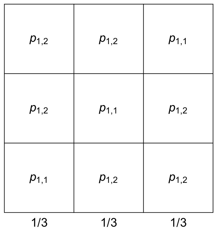 Figure 1
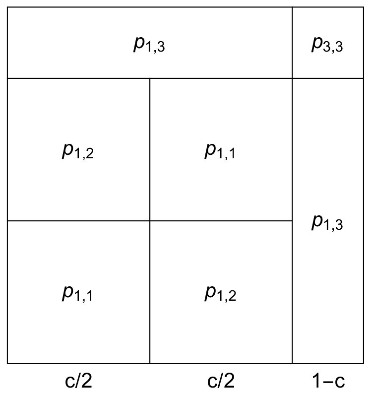 Figure 2
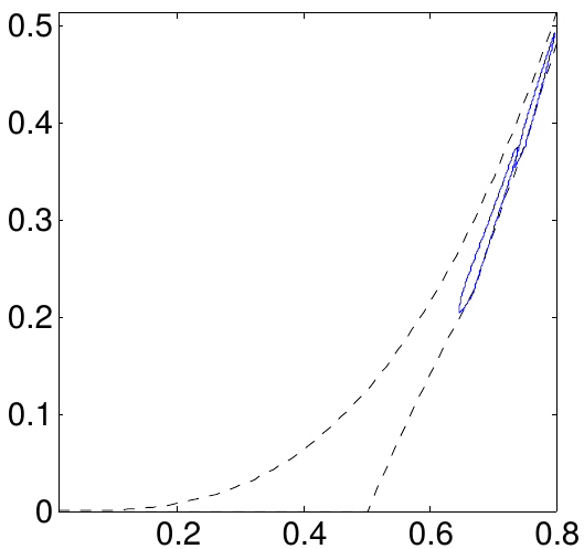 Figure 3
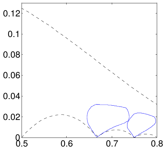 Figure 4
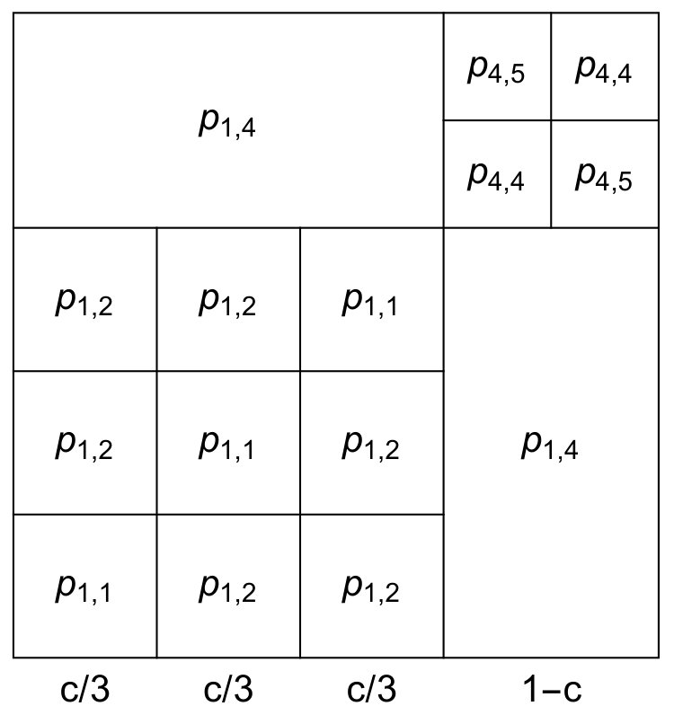 Figure 5
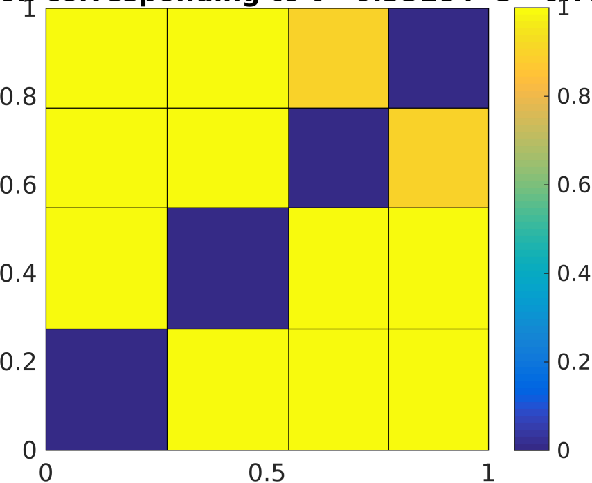 Figure 6
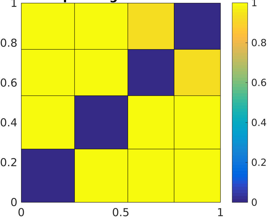 Figure 7
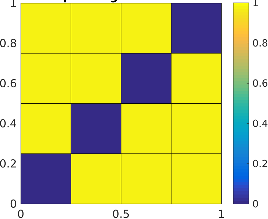 Figure 8
 Figure 9
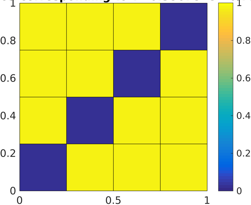 Figure 10
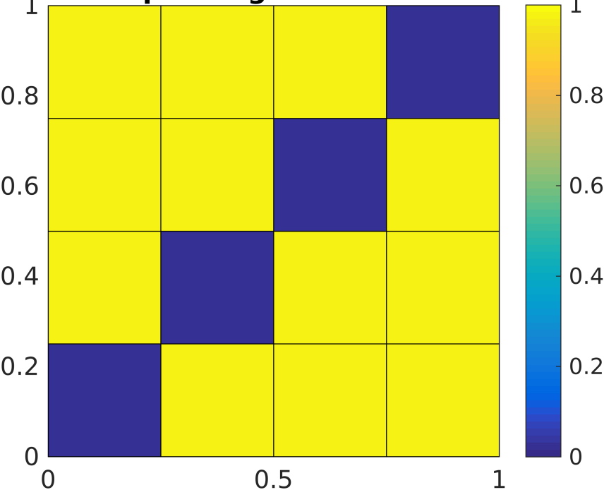 Figure 11
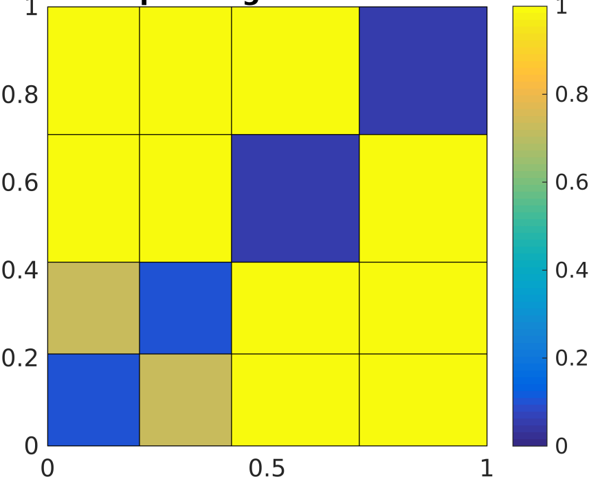 Figure 12
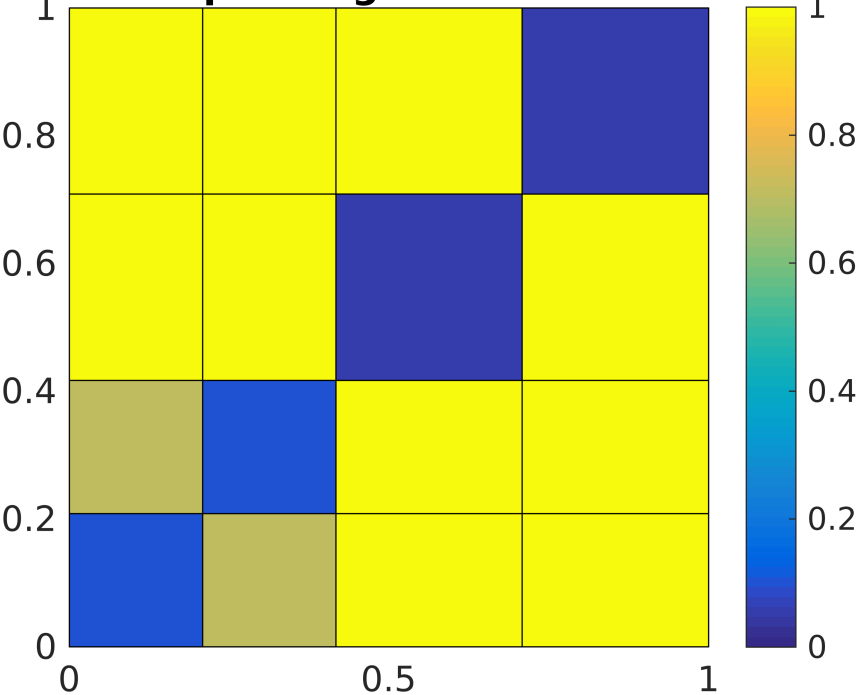 Figure 13
 Figure 14
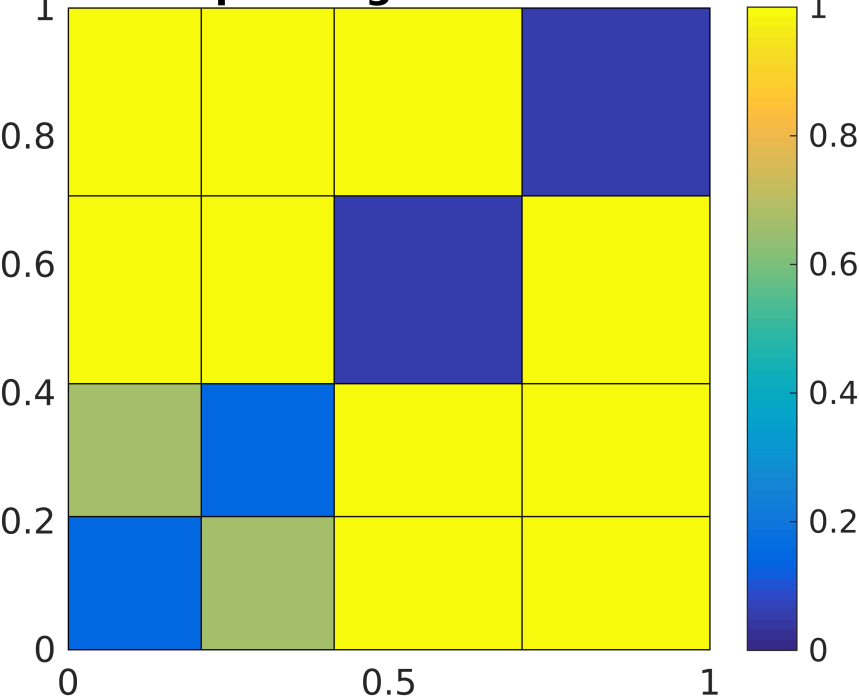 Figure 15
 Figure 16
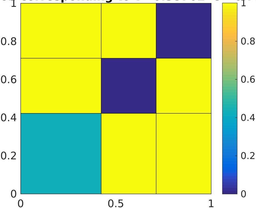 Figure 17
 Figure 18
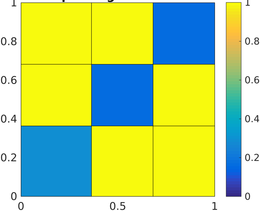 Figure 19
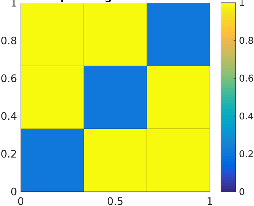 Figure 20
 Figure 21
 Figure 22
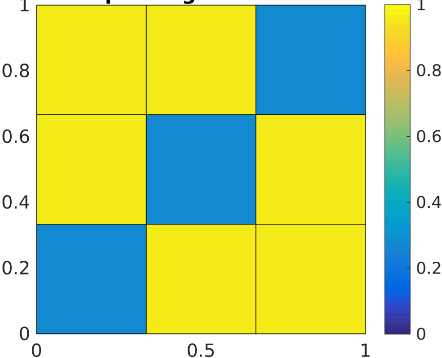 Figure 23
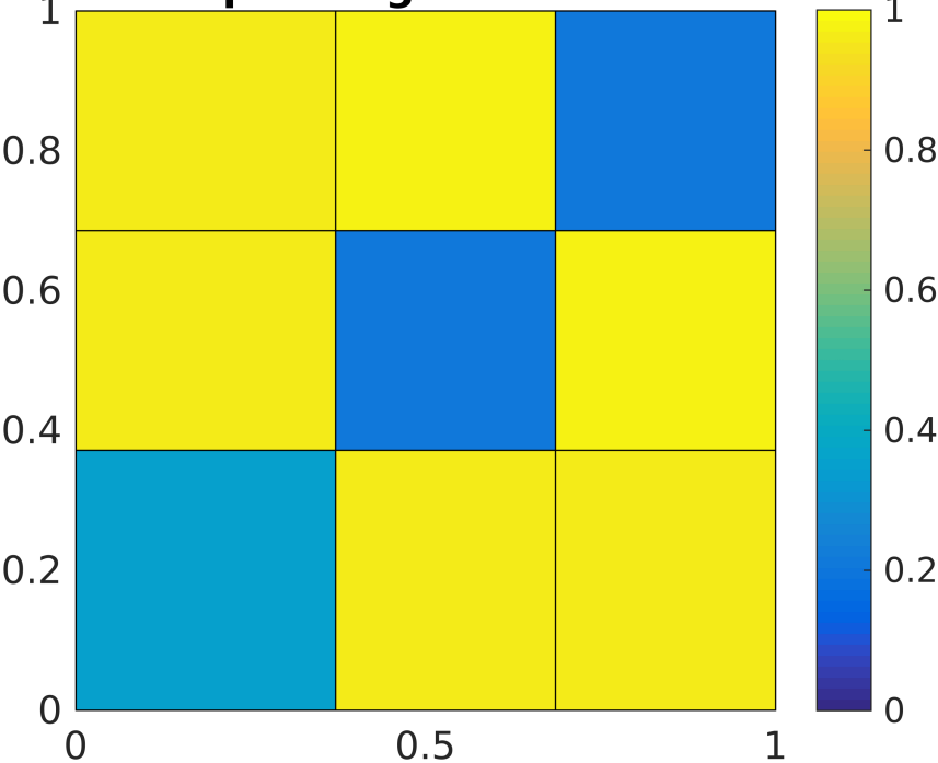 Figure 24
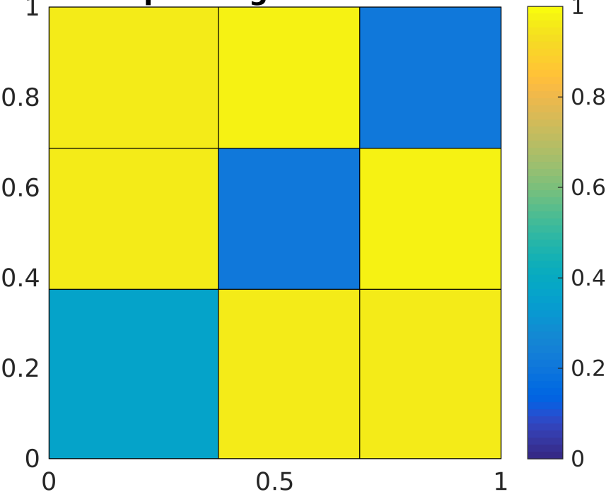 Figure 25
 Figure 26
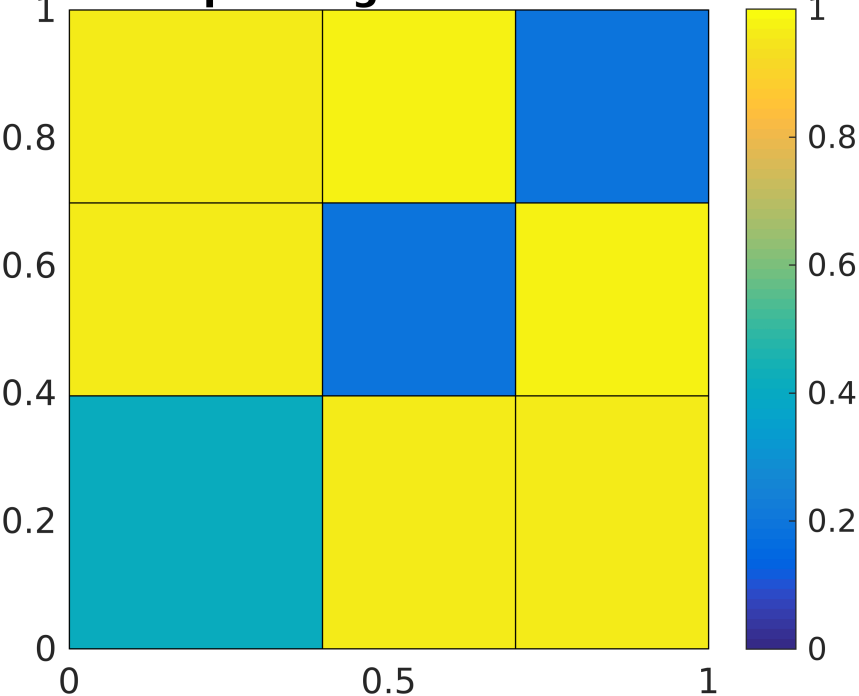 Figure 27
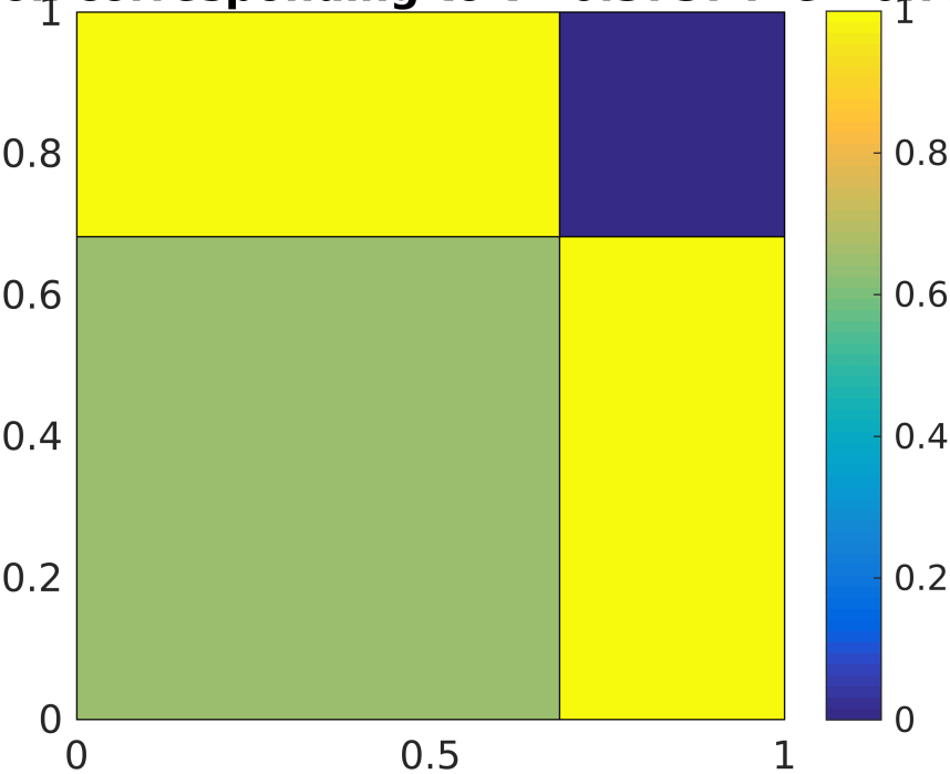 Figure 28
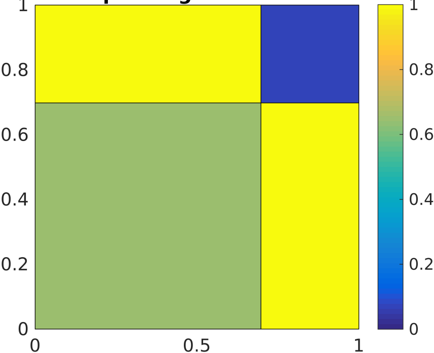 Figure 29
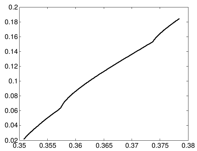 Figure 30
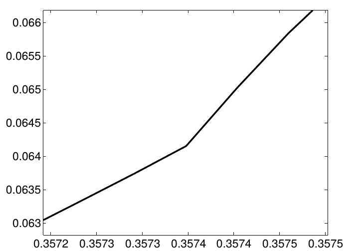 Figure 31
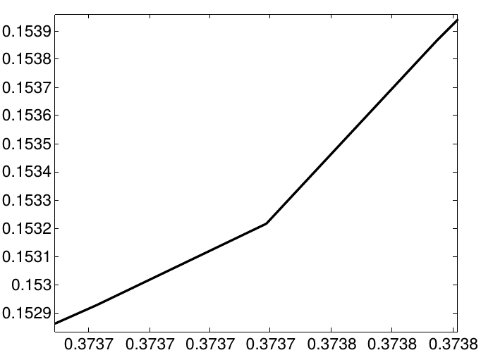 Figure 32
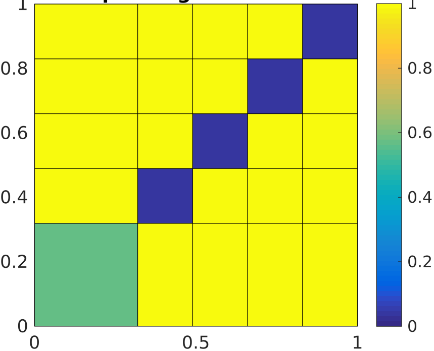 Figure 33
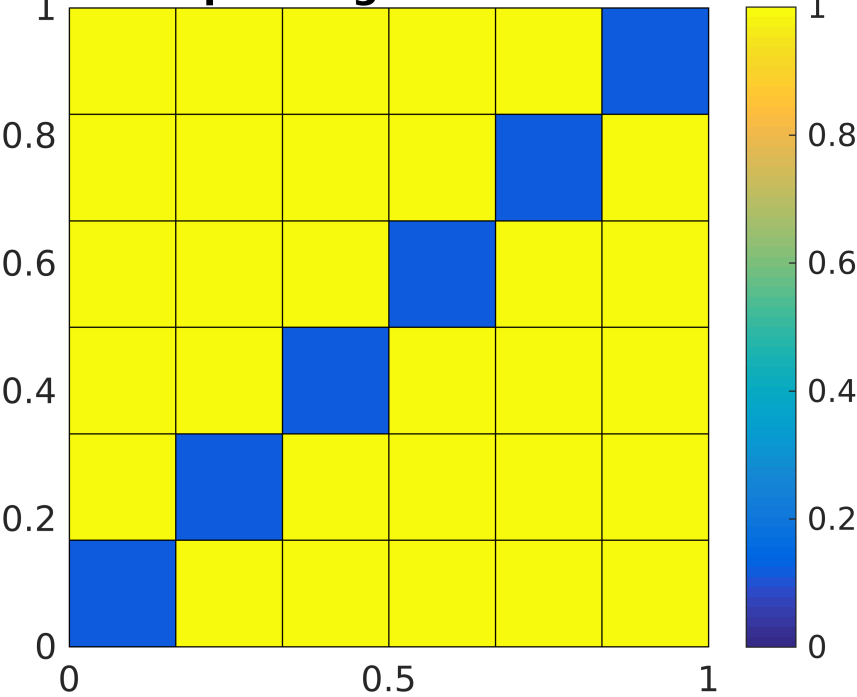 Figure 34
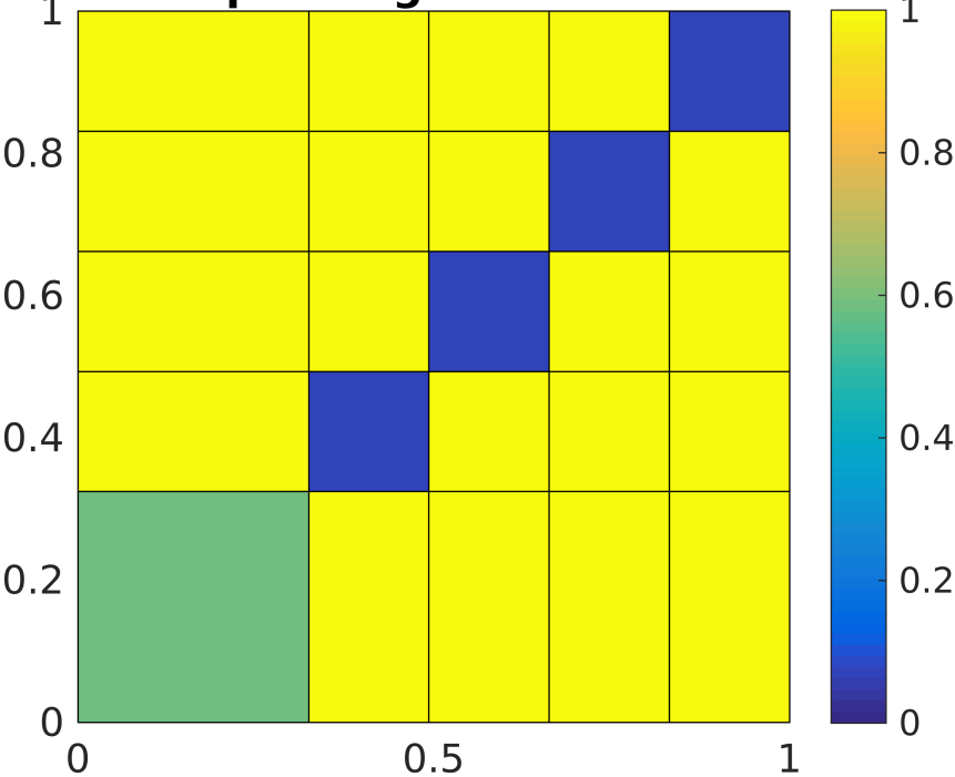 Figure 35
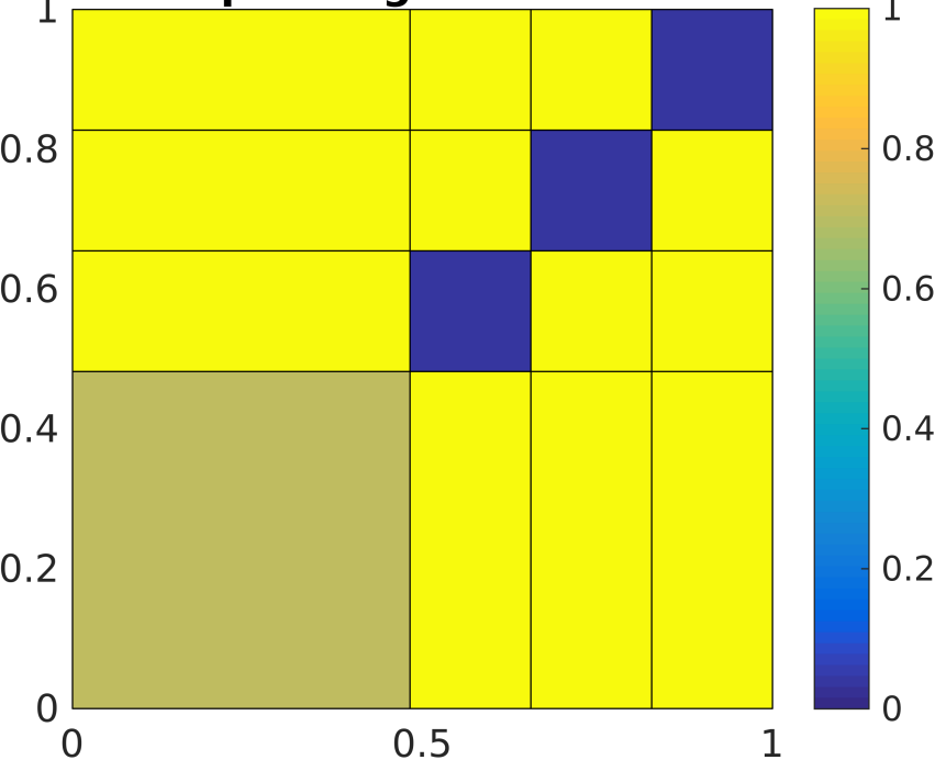 Figure 36
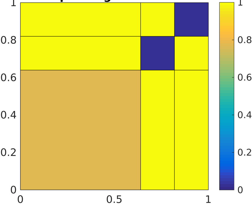 Figure 37
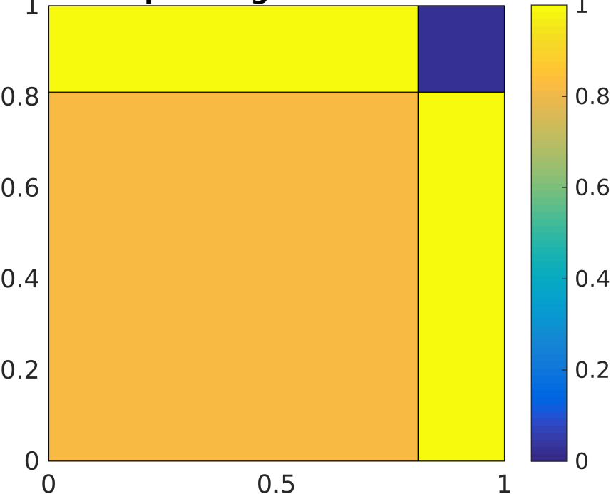 Figure 38
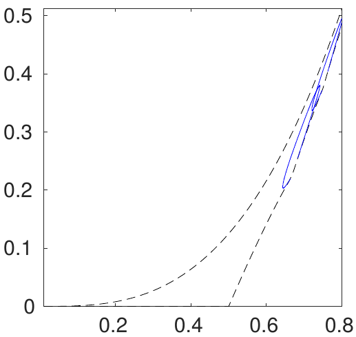 Figure 39
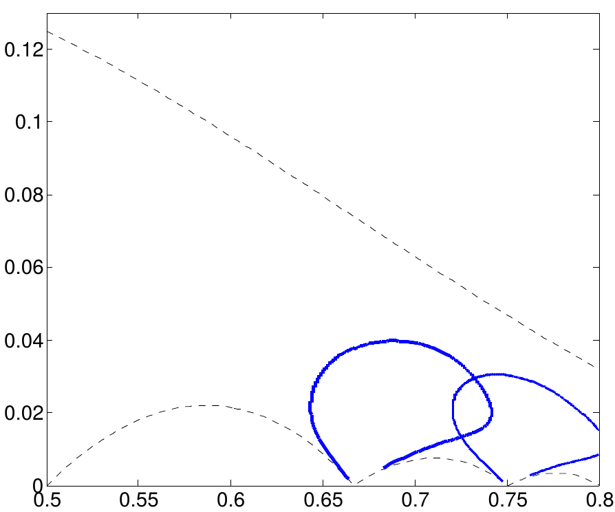 Figure 40
Peer Reviews
No public reviews on file for this paper yet. If you reviewed it on a platform where reviews are public (OpenReview, ICLR, NeurIPS, ICML), you can paste yours below so the community can read it here.
Videos
No videos yet. Explain this paper in a talk, walkthrough, or lecture? Add one.
The phases of large networks with
edge and triangle constraints
Richard Kenyon Department of Mathematics, Brown University, Providence, RI 02912; [email protected]
Charles Radin Department of Mathematics, University of Texas, Austin, TX 78712; [email protected]
Kui Ren Department of Mathematics, University of Texas, Austin, TX 78712; [email protected]
Lorenzo Sadun Department of Mathematics, University of Texas, Austin, TX 78712; [email protected]
Abstract
Based on numerical simulation and local stability analysis we describe the structure of the phase space of the edge/triangle model of random graphs. We support simulation evidence with mathematical proof of continuity and discontinuity for many of the phase transitions. All but one of the many phase transitions in this model break some form of symmetry, and we use this model to explore how changes in symmetry are related to discontinuities at these transitions.
1 Introduction
We use the variational formalism of equilibrium statistical mechanics to analyze large random graphs. More specifically we analyze “emergent phases”, which represent the (nonrandom) large-scale structure of typical large graphs under global constraints on subgraph densities. We concentrate on the model with edge and triangle density constraints, and , which in this context play somewhat similar roles that mass and energy density constraints play in microcanonical models of simple materials. Our goal is to understand the statistical states which maximize entropy for given and . These are the analogues of Gibbs states in statistical mechanics.
Other parametric models of random graphs are widely used, in particular exponential random graph models (analogues of grand canonical models of materials), and the edge/triangle constraints have been studied in that formalism since they were popularized by Strauss in 1986 [21]. (There is a short discussion of exponential models in Section 2.)
This paper, following on [13, 14, 15, 4, 5, 16], is the first attempt to determine the qualitative features of the whole phase space of the edge/triangle model. We discuss what phases exist, and give the basic features of the transitions between these phases; see Figure 1.
The phase space is the space of achievable values of the constraints, and a phase is a connected open subset of in which the entropy optimizing are unique for given , and vary analytically with . In the case of edge/triangle constraints is the “scalloped triangle” of Razborov [17] (see Figure 2).
Determining the optimal states in the edge/triangle model is a difficult variational problem, one that has not been solved rigorously except in special regions of the phase space [13, 14, 15, 4, 5, 16]. However there is solid evidence that each individual optimizer is multipodal, that is, described by a stochastic block model (see definition below). This evidence is borne out by our numerical studies, and based on them we conjecture that the optimal states occur in three families (plus one extra phase), corresponding to certain equivalences or symmetries, as follows. We will give the evidence for our conjectures as we proceed.
In the region of there are three infinite families of phases, denoted , and ; See Figure 1. Each statistical state in an phase corresponds to a partition of the set of nodes into subsets which are equivalent in the sense that the sizes of all are of the whole, the probability of an edge between and is independent of and , only depending on whether or . It follows that for an phase there are only two statistical parameters and , which are thus easily computable functions of the edge and triangle constraints, and . See for example Figure 3 for the case , and the left graphon in Figure 4.
The phase touches the lower boundary of at the cusp .
A statistical state in a phase corresponds to a partition of into statistically equivalent subsets, , plus one other set of statistically equivalent nodes, see Figure 4 middle. In the phase diagram, these phases are arranged in stripes coming out of the point , and part of the boundary of is shared with and with . These are depicted schematically in Figure 1.
A statistical state in a phase corresponds to a nodal partition into equivalent subsets, , plus another statistically equivalent pair of subsets, see Figure 4 right. The phase shares boundary with , , and the scallop connecting the cusps with and . See Figure 1.
denotes the single phase for the region ; see Figure 1. A statistical state in corresponds to a bipodal graphon. Although this is the same basic structure as , the two phases are different in more subtle ways.
The multipodal structure of the has only been proven on certain subsets of the phase space: on the boundary, on the Erdős-Rényi curve , on the line segment for , and in a region just above the Erdős-Rényi curve; see [5]. It has however also been proven just above the Erdős-Rényi curve in a wide family of other models [5], for all parameters in edge/-star models [4], and is supported in our edge/triangle model by extensive simulations for a range of constraints [15].
The support for the specific pattern of phases in Figure 1 is purely from simulation and will be described in Section 3.
In Section 4 we use this detailed structure of the optimal states to analyze the transitions between phases. In our edge/triangle model all phase transitions involve a change of symmetry. Some of the transitions are continuous and some discontinuous, and we prove some of these results in that section. The role of symmetry in determining these qualitative features is of interest, given the major role that symmetry plays in the understanding of phase transitions in statistical physics [8, 1]. We discuss this further in Section 5.
2 Notation and formalism
The study of large dense graphs uses the mathematical tool of graphons, which we now review [6], making use of the discussion in [12]. We let denote the set of graphs on nodes, which we label . Graphs are assumed simple, i.e. undirected and without multiple edges or loops. A graph in can be represented by its -valued adjacency matrix, or alternatively by the function on the unit square with constant value 0 or 1 in each of the subsquares of area centered at the points ; see Figure 5.
More generally, a graphon is an arbitrary symmetric measurable function on with values in . We define the “cut metric” on graphons by
[TABLE]
Informally, is the probability of an edge between nodes and , and so two graphons are called equivalent if they agree up to a ‘node rearrangement’, that is, where is a measure-preserving transformation of (see [6] for details). The cut metric on graphons is invariant under the action of : . We define the cut metric on the quotient space of ‘reduced graphons’ to be the infimum of (1) over all representatives of the given equivalence classes. is compact in the topology induced by this metric [6].
We now consider the notion of ‘blowing up’ a graph by replacing each node with a cluster of nodes, for some fixed , with edges inherited as follows: there is an edge between a node in cluster (which replaced the node of ) and a node in cluster (which replaced node of ) if and only if there is an edge between and in . Note that the blowups of a graph are all represented by the same reduced graphon, and can therefore be considered a graph on arbitrarily many – even infinitely many – nodes, which allows us to reinterpret Figure 5 as representing a multipartite graph. This represents a form of symmetry which we exploit next, and discuss in Section 5.
The ‘large scale’ features of a graph on which we focus are the densities with which various subgraphs sit in . Assume for instance that is a -cycle. We could represent the density of in in terms of the adjacency matrix by
[TABLE]
where the sum is over distinct nodes of . For large this can approximated, within , as:
[TABLE]
It is therefore useful to define the density of this in a graphon by
[TABLE]
The density for other subgraphs is defined analogously. We note that only depends on the equivalence class of and is a continuous function of with respect to the cut metric on reduced graphons. It is an important result of [6] that the densities of subgraphs are separating: any two reduced graphons with the same values for all densities are the same.
Our goal is to analyze typical large graphs with variable edge/triangle constraints in the phase space of Figure 2. Our densities are real numbers, limits of densities which are attainable in large finite systems, so we begin by softening the constraints, considering graphs with nodes and with edge/triangle densities satisfying and for some small (which will eventually disappear.) It is easy to show that the number of such constrained graphs is of the form , for some and by a typical graph we mean one chosen from the uniform distribution on the constrained set.
Getting back to our goal of analyzing constrained uniform distributions, a related step is to determine the cardinality of the set of graphs on vertices subject to the constraints. Constraints are expressed in terms of a vector of values of a set of densities, and a small parameter . Denoting the cardinality by , it was proven in [13, 14] that exists; it is called the constrained entropy . As in statistical mechanics this can be usefully represented via a variational principle.
Theorem 2.1
(The variational principle for constrained graphs [13, 14]) For any -tuple of subgraphs and -tuple of numbers,
[TABLE]
where is the graphon entropy:
[TABLE]
Variational principles such as Theorem 2.1 are well known in statistical mechanics [18, 19, 20]. One aspect of such a variational principle in the current context is not well understood, and that is the uniqueness of the optimizer. In all known graph examples the optimizers in the variational principle are unique in except on a lower dimensional set of constraints where there is a phase transition. Assuming there is a unique optimizer for (5), this optimizer is the limiting constrained uniform distribution. We will discuss the question of uniqueness of entropy optimizers in Section 5.
Finally we contrast the above formalism with the formalism of exponential random graph models (ERGM’s) mentioned in the Introduction. The latter are widely used, especially in the social sciences, to model graphs on a fixed, small number of nodes [10]. They are sometimes considered as Legendre transforms of the models being discussed in this paper [13]. However, as was pointed out in [2], this use of Legendre transform is largely problematic, since the constrained entropy in these models is neither convex nor concave, and the Legendre transform is therefore not invertible [13]. As a consequence the parameters in ERGM’s become redundant, and this confuses any interpretation of phases or phase transitions in such models.
3 Numerical simulation
We now briefly describe the computational algorithms that we used to obtain the phase portrait sketched in Figure 1. The details of the algorithms, as well as their benchmark with known analytical results, can be found in [15]. In the algorithms, we assume that the entropy maximizing graphons are at most -podal, the largest number of podes that our computational power can handle. We then draw random samples from the space of -podal graphons, select those that satisfy, besides the symmetry constraints, the constraints on edge and triangle densities up to given accuracy. We compute the entropy of these selected graphons and take the ones with maximal entropy as the optimizing graphons.
For each given value, we generate a large number of samples such that the optimizing graphons we obtain have entropy values that are within a given accuracy to the true values. The computational complexity of such a procedure is extremely high for high accuracy computations. For each optimizing graphon which we determined with the sampling algorithm, we use it as the initial guess for a Netwon-type local optimization algorithm, more precisely a sequential quadratic programming (SQP) algorithm, to search for local improvements. Detailed analysis of the computational complexity of the sampling algorithm and the implementation of the SQP algorithm are documented in [15]. The results of the SQP algorithms are the candidate optimizing graphons that we show in the rest of this section.
The phase boundaries.
In the first group of numerical simulations we try to determine the boundaries of two of the completely symmetric phases, the phase and the phase. As we pointed out in the Introduction, for a given value in we know analytically the unique expression for the optimal graphon (see, for instance, equation (28)) and the corresponding entropy. Therefore, a given point is outside of the phase if we can find a graphon that gives a larger entropy value, and is within the phase if we can not find a graphon that has a larger value. We use this strategy to determine the boundaries of the and the phases. In Figure 6 we show the boundaries we determined numerically. Note that since these boundaries are determined using a mesh on the plane, they are only accurate up to the mesh size in each direction. For better visualization, we reproduced Figure 6 in a rescaled coordinate system, , in Figure 7.
Phases along line segment .
In the second group of numerical simulations, we provide some numerical evidence to support our conjecture on phases depicted in Figure 1. Consider the optimizing graphons in the phases which the vertical line segment : , cuts through. (Figure 1 is quite crude: for an accurate representation of the boundaries of and see Figure 6 .) From top to bottom, the line cuts through: , , , , , , and phases. In Figure 8, we show the optimizing graphons in phases before and after each transition along the line. Let us mention here two obvious discontinuous transitions, the first being the transition from to at about , and the second being the transition from to at about . The derivative of the entropy with respect to exhibits jumps at these transitions, as seen in Figure 9. A theoretical analysis of the transitions is presented in the next section.
Phases along line segment .
We performed similar simulations to reveal phases along the line segment , . The phases, from top to bottom, should be, respectively , , , , , , , and . Our simultation did not capture the last two phases, which lie extremely close to the lower boundary of the phase space; representive optimizing graphons for the others are shown in Figure 10. Also, due to limitations in computational power we were not able to resolve the transitions between the phases as accurately as in the previous case, that is, those in Figure 8.
Remark on our conjecture on the phase space structure.
We now briefly summarize the evidence behind our conjecture of the phase portrait in Figure 1. First of all, by simulations and proofs in several models, in particular this one, we had found that in the interior of phase spaces optimizing graphons have always been found to be multipodal. In this model furthermore, the only place we find more than 3 podes is for and near the scalloped boundary. (Recall that in all the numerical simulations in this paper we assume that the graphons have or fewer podes, even though where we simulate they always end up having many fewer than podes). Second, for each point in the phase space except for and close to the scallops), our algorithm, even though computationally expensive, could determine the optimal graphons up to relatively high accuracy. The computational cost is in general tolerable; in the exceptional region it is too expensive to find enough graphons which satisfy all the constraints to get the accuracy we wanted. (In more detail, we use the techniques explained in [15] with edge and triangle constraint intervals of size , which determines entropy to order , from which we determine our optimal graphons.) Third, within each phase away from the scallops our computational power allows us to perform simulations on relatively fine meshes of . This is how we determined the boundary of the and phases as well as the transitions shown in Figure 9, for instance. In more detail, consider the middle two graphons in each row in Figure 8, which straddle the transitions. They all have edge density . In the first row they have triangle densities and ; in the second row the triangle densities are and ; in the third row they are and ; in the fourth row they are and ; in the fifth they are and ; and in the last row they are and .
4 Analysis of transitions
As noted above, the numerical simulations indicate that all phase transitions below the Erdős-Rényi curve with the exception of , occur discontinuously. At each other transition, the optimizing graphon jumps from one form to another, and so the densities of certain subgraphs also jump. In this section, we prove that certain of these transitions can only occur discontinuously.
Theorem 4.1
Except at a finite number of values of the edge density , there cannot be a continuous transition from a bipodal phase to a or tripodal phase.
Theorem 4.1 can be generalized to consider all transitions:
Theorem 4.2
Except at a finite number of values of the edge density , there cannot be a continous transition from a to a phase.
Assuming that our conjectured phase portrait is correct, this leaves the , , and transitions for us to consider.
Theorem 4.3
For , there cannot be a continuous transition from a phase to a phase, and there cannot be a continuous transition from an phase to a phase.
To summarize (see Figure 1) we have proven that transitions cannot be continuous between: any two phases; any and phases; any and phases except perhaps at finitely many values of . As noted earlier, transitions between and phases appear to always be discontinuous, and transitions between any and phases appear to always be continuous. However, we currently lack a proof for these last two claims, although in [16] there is a possible path to prove continuity for .
For completeness we note that the two transitions across the Erdős-Rényi curve, and , are continuous: for on the Erdős-Rényi curve the graphon with constant value is easily seen to be the unique entropy-optimizer, and the optimizers from each side must approach it in and therefore in cut metric.
Proof of Theorem 4.1. The phase is in the family and appears to the left of the phase, while is in the family and appears to the right of . For purposes of this proof, however, they are indistinguishable. All that matters is that there are three “podes”, with a symmetry swapping two of them.
The proof has three steps:
Showing that the Lagrange multipliers (see definition below) would have to diverge at a continuous transition. 2. 2.
Showing that for a bipodal optimizing graphon, divergent Lagrange multipliers can only occur at the “natural boundary” of the phase, namely at the minimum possible value of achievable by a bipodal graphon for the given value of . 3. 3.
Showing that on the natural boundary, there exists a tripodal graphon with the given values of and with higher entropy than any bipodal graphon. That is, showing that the natural boundary of the phase actually lies within a tripodal phase. This step requires that a certain analytic function of be nonzero. Since analytic functions (that aren’t identically zero) can only have finitely many roots in a compact interval, this step of the proof can break down at finitely many values of . (Numerical examination of the analytic function reveals that it does not have any roots at all for relevant values of , making the “all but finitely many” caveat moot in practice.)
We establish some notation. For any graphon , we let and denote the densities where is an edge and a triangle, respectively. For our graphon, we let
[TABLE]
and let be the size of the first pode. For a graphon, we assume that the first two podes are interchangable, each of size , and set , , , and . That is, the graphon is obtained from a graphon by splitting the first pode in half (and renumbering the last pode), and by making and distinct variables. The only way that a graphon can be a limit of graphons is if goes to zero (note that if it becomes a type graphon, not a ). So to prove our theorem, we must show that a sequence of entropy maximizers cannot approach a limiting graphon with .
The Euler-Lagrange equations for maximizing entropy (see [4]) say that there exist constants and such that, for all ,
[TABLE]
or more explicitly
[TABLE]
where
[TABLE]
For a graphon, the integral equals
[TABLE]
The Lagrange multiplier equals and is always positive, since we can increase both the entropy and by linearly interpolating between our given graphon and a constant graphon.
Subtracting equation (9) for from equation (9) for gives:
[TABLE]
By the mean value theorem, the left hand side equals for some between and , and so
[TABLE]
Since and is negative and bounded away from zero, must be greater than and must diverge to as approaches zero. To compensate, must diverge to . This completes step 1.
To understand the effect of divergent Lagrange multipliers, we must consider all of the variational equations for bipodal graphons, including those related to changes in . The edge, triangle and entropy densities are:
[TABLE]
Taking gradients with respect to the four parameters and setting gives the four equations:
[TABLE]
Note that the left hand side of the third equation is always finite, and that the left hand sides of the other equations only diverge if the relevant parameter , , or approaches 0 or 1. Otherwise, in the limit the ratios of the coefficients of and must be the same for all equations. In other words, there is a constant such that
[TABLE]
where we restrict attention to parameters that are not 0 or 1, and such that a parameter equals 0 if and equals 1 if . (The signs of the inequalities come from the sign of as or .)
However, these are precisely the same equations that describe finding a stationary point for for fixed , without regard to the entropy. For graphons, such stationary points occur only for Erdős-Rényi graphons, with , or for minimizers of , with and and satisfying the algebraic condition
[TABLE]
This completes step 2.
Finally, we must show that a graphon with and , and satisfying (23), is not an entropy maximizer. Among bipodal graphons with and and a fixed value of , minimizing and minimizing the entropy give different analytic equations for and . For all but finitely many values of , these equations have distinct roots, implying that the graphon that minimizes does not maximize the entropy. If we start at the bipodal graphon that minimizes for fixed and change to , while adjusting to keep fixed, we can increase the entropy to first order in while only increasing to second order in .
To compensate for this increase in , we can split the first pode in half, yielding a tripodal graphon with and , with and . This decreases by , while decreasing the entropy by . By taking to be of order , we can restore the initial value of at an entropy cost of .
For sufficiently small and of the correct sign, the gain in entropy from changing and is greater than the cost in entropy from having , so the resulting graphon has higher entropy, but the same values of and , than the graphon that minimizes (among graphons). This completes step 3.
Proof of Theorem 4.2. The proof follows the same strategy as that of the case. In step 1 we show that the Lagrange multipliers must diverge at a continuous transition. In step 2 we show that divergent Lagrange multipliers force a graphon to be a stationary point of for fixed . In step 3 we show that we can perturb such a stationary graphon into a graphon with the same values of and more entropy, implying that we are not actually at the phase boundary, which is a contradiction.
We parametrize graphons as follows: There are two interchangable podes, each of size , and podes of size . Let denote the value of when is in the -th pode and is in the -th. We define parameters such that
[TABLE]
The transition that we are trying to rule out is one where approach a common value , resulting in a graphon with one pode of size and podes of size , with
[TABLE]
Let , and be the gradients of the functionals , and with respect to the parameters or , depending on the phase we are considering. Maximizing the entropy for fixed means finding Lagrange multipliers and such that
[TABLE]
In the phase, one checks that is first order in , while is second order. This forces to diverge to as , which in turn forces to diverge to , exactly as in the proof of Theorem 4.1. This concludes step 1.
Next we consider equation (26) in the limit of divergent and . Restricting attention to those parameters for which does not diverge (i.e. those that are not 0 or 1 in the limiting graphon), we have that and must be collinear. That is, there is a constant such that, for each parameter taking values in , we must have that . Furthermore, if in the limit goes to 0 we must have and if approaches 1 we must have . That is,
[TABLE]
where we restrict attention to parameters that are not 0 or 1, and we have 1-sided inequalities for those remaining parameters. This is precisely the set of equations obtained by ignoring entropy and looking for stationary points of for fixed , with being the Lagrange multiplier of this process. Seeking entropy maximizers with divergent is equivalent to seeking stationary points of for fixed . This concludes step 2.
Now we consider a 1-parameter family of graphons, with a fixed value of , that satisfy all of (27) except the equation relating and . Since by assumption we start at a stationary point of , moving along this family will only change to second order or slower in the change in , but for all but finitely many values of will change to first order. Move a distance in the direction of increasing . A priori we do not know that the resulting change in will be positive, but negative changes in can be compensated for while increasing , since is positive. If the change in is positive, then we can compensate by splitting the first pode in half, with of order , restoring at an entropy cost of . Since , by picking small enough we can always find a graphon that does better than the graphon that was purportedly the entropy maximizer at the phase boundary, which is a contradiction.
Proof of Theorem 4.3. This proof does not require any consideration of entropy. The symmetries are simply incompatible, in that there is no way to approximate a graphon with a graphon, and there is no way to approximate a graphon with an graphon.
We now turn to determining the locations of the phase transitions. For each of the discontinuous transitions, this is a difficult problem. The optimizing graphons on each side of the transition line are very different, so it is impossible to use perturbation theory to understand the behavior near the line. Instead, one must study each phase separately and approximate the entropy in each phase as an analytic funciton of and (e.g., by doing a polynomial fit to numerical data). These functions can then be continued over a larger region and compared. The phase transition line is the locus where the two functions are equal. Using such techniques, we can localize the transition lines and the triple points with considerable accuracy, but in the end the results remain grounded in numerical simulation, and cannot provide independent confirmation of our numerics.
For the continuous transitions, however, it is possible to obtain an analytic equation satisfied along the transition line. This was already done for the transition in [15, 16]. Here we extend the results to .
This calculation, although elementary, is too long to present here in its entirety; we give the method here. For each fixed , the space of graphons is 5-dimensional. As in Figure 3, we imagine intervals of size and one of size , and must specify , , , and . An graphon is a special case of this with , and , and for such graphons the parameters and are easily computed from the edge and triangle densities:
[TABLE]
Returning to a general graphon, we use the constraints on and to eliminate two variables, expressing as functions of : . In fact we don’t need to solve explicitly; we only need the first and second partial derivatives of (evaluated at the parameter values of the graphon), which can be obtained by implicit differentiation of the equations for . Then the entropy is a function of : Computing its Hessian at the phase when yields the matrix
[TABLE]
where . Within the phase, this second variation is negative-definite, while within the phase the matrix has a positive eigenvalue. The boundary is thus defined (locally) by the analytic equation .
One can also consider continuous changes from an graphon to a graphon with a symmetry other than . The local stability condition for such changes works out to be exactly the same as for . The upshot is that the analytic curve defines the boundary of the region where the graphon is stable against small perturbations.
In Figure 11 we plot the regions where the and graphons are stable against small perturbations. Comparing to Figures 6 and 7, we see that the stability regions are larger than the actual and phases, and even overlap! Without assuming anything about the phase portrait (beyond the existence of and phases) this proves that some of the transitions from or to other phases must not be governed by the local stability condition, and so must be discontinuous.
The transition is a supercritical pitchfork bifurcation [16]. The analytic family of entropy maximizers in the phase has a natural analytic continuation into the region, but no longer maximizes entropy there. The analytic family of entropy maximizers in the phase doubles back on itself and cannot be continued into the region. Power series analysis suggests that something similar happens in the transition from to . The family of graphons representing entropy maximizers can be continued into the region but no longer maximizes entropy. The family of graphons representing cannot be analytically continued into the region, but instead doubles back into the region. Unlike in the case of , the “doubling back” branch is not related by symmetry to the original branch, and so represents a different set of reduced graphons, all stationary points of the entropy, but with presumably lower entropy than graphons of the original branch with the same values of .
It is a classical result (Mantel’s theorem [9], generalized by Turán [22]) that the only way to satisfy the constraints of edge density and triangle density is with the complete, balanced bipartite graph, which implies that those values of those density constraints determine the values of the densities of all other subgraphs. Put another way, there is a unique reduced graphon with and . Likewise, for each there is a unique reduced graphon with the maximum possible value of . This phenomenon is called ‘finite forcing’; see [7]. However, this phenomenon only occurs on the boundary of the phase space:
Theorem 4.4
For each pair in the interior of the space of achievable values (see Figure 2), there exist multiple inequivalent graphons with and .
Proof: For fixed , let be a graphon that minimizes given , and let be a graphon that maximizes , and let be a general measure-preserving homeomorphism. The graphon is always -podal for some , while is bipodal. For , let . This will be a multipodal graphon, generically with podes whose sizes depend on the details of but not on the value of . In particular, we can choose homeomorphisms and such that the podal structure of is different from that of , and hence is different from that of for arbitrary .
It is easy to check that , and that for given , is a continuous function of . By the intermediate value theorem, we can thus find graphons and such that and . But and have different podal structures, and so are inequivalent.
In contrast to the graphons not being determined by and , simulations indicate that maximizing the entropy for fixed does give a unique reduced graphon throughout the interior, except on a lower dimensional set, the exceptions being constraint values associated with the discontinuous phase transitions. (The uniqueness of the entropy maximizer was also proven analytically for for any in [13], and for an open subset of the phase in [5].) We do not yet have a theoretical understanding of this fundamental issue, sometimes called the Gibbs phase rule in physics; see however [4] for -star graph models, and [19, 3] for weak versions in physics.
5 Symmetry
All aspects of this paper relate to the symmetry of phases, referring to the symmetry of the unique entropy-optimizing graphons for points in the phase. These symmetries occur at two levels.
The first and most significant level of symmetry is a consequence of the multipodality of the , which means that the set of all nodes is composed of a finite number of equivalence classes: the probability of an edge, between a node in class with a node in class , is independent of and , only depending on and .
The second level of symmetry concerns the equivalence classes of nodes: certain equivalence classes have the same sizes and edge probabilities, and others don’t. These size and probability parameters are used to distinguish distinct phases, that is, maximal open regions in the parameter space where the entropy-maximizing graphon is unique and varies analytically.
Because of multipodality the function restricted to a given phase can be considered a smooth vector valued function of , the coordinates being the probabilities of edges between node equivalence classes, and the relative sizes of those equivalence classes. By the symmetry of a phase we refer to the symmetries among these coordinates, with the following caveat, illustrated through an example. Within the phase there is a curve such that the two node equivalence classes have the same size. In a narrow sense this might have signalled a higher symmetry. However there is no singular behavior as crosses this curve so the curve is simply part of and does not affect the ‘symmetry’ of the phase.
Each of the phases has a different symmetry and we conjecture that they all fall into the three families: , and , or , in which the notation completely specifies the symmetry (except for the pairs , and ).
An important result of this paper is the conjectured phase diagram, Figure 1. The other goal is to show how knowledge of the structure of optimizing graphons in phases can be helpful in understanding the role of symmetry in specific features of phase transitions. Consider the following, paraphrased from P.W. Anderson [1], a picture he attributes to Landau [8]:
The First Theorem of solid-state physics states that it is impossible to change symmetry gradually. A symmetry element is either there or it is not; there is no way for it to grow imperceptibly.
This intuitive picture has been applied, for instance by Landau, to understand why there is no critical point for the fluid/solid transition [1], though it has been difficult to make the argument rigorous:
This is the theoretical argument, which has appeared to some to be a little too straightforward to be absolutely convincing [11].
We suggest that network models such as the edge/triangle model of this paper provide a useful framework for enabling a rigorous study of such symmetry principles. This was done in [16] specifically for the issue of existence of a critical point.
Landau’s symmetry principles are commonly applied to the issue of whether phases are continuous at a transition [8], which is also related to uniqueness of entropy optimizers.
We have proven that in the edge/triangle model certain transitions cannot be continuous, and evidence suggests that certain other transitions are continuous. It is worthwhile discussing how these transitions are approached at the micro-level, that is, in terms of the multipodal parameters, the probabilities of edges between various type of nodes. In this regard Figure 1 and Figure 8 are useful.
For all the discontinuous transitions, those proven and those only seen in simulation, we believe from simulation that the transitions can be visualized as the intersection of a pair of two dimensional smooth surfaces both of which exist beyond the intersection but only represent entropy-optimizers on one side. See rows in Figure 8.
For the continuous transitions there is more variety. By simulation the continuous transition is achieved through directly acquiring the higher symmetry of . See rows and in Figure 8. An analogue in statistical mechanics would be a transition between crystal phases in which a rhombohedral unit cell becomes, and remains, cubic. On the other hand the transition occurs by the different bipodal symmetries on both sides rising to the full symmetry of the constant graphons at the Erdős-Rényi curve. It is noteworthy that the full symmetry of the constant graphon is incompatible with any possible phase in our sense: since , there is not a two-dimensional family of parameter values.
6 Conclusion
The edge/triangle model in this paper was built by analogy with microcanonical mean-field models in statistical mechanics. Mean-field models are useful because frequently the free energy can be determined analytically as a function of the thermodynamic parameters. An important distinction for the edge/triangle and related random graph models is that not only the free energy (entropy in this case) but also the entropy-optimizing graphons (which are the analogues of the Gibbs states) can sometimes be determined for a range of parameters. For instance in [16, Section 3.7] this control of the optimizing states is used to compute how some global quantity changes with the constraint parameters, a level of analysis never possible in short or mean-field models in statistical mechanics.
The main result of this paper is the conjectured phase diagram, Figure 1, for edge/triangle constraints, based largely on simulation, including continuity/discontinuity of all the transitions and the structure of the entropy-optimizing states within each phase.
The secondary goal is to show how knowledge of the structure of the optimizing graphons can be helpful in understanding the role of symmetry in the continuity/discontinuity of phase transitions.
Interesting subjects for further investigation include the triple points where phases , and meet, all the pairwise transitions being continuous, and where , and meet, with and discontinuous and continuous.
Acknowledgments
The main computational results were obtained on the computational facilities in the Texas Super Computing Center (TACC). We gratefully acknowledge this computational support. This work was also partially supported by NSF grants DMS-1208191, DMS-1612668, DMS-1509088, DMS-1321018 and DMS-1620473, and Simons Investigator grant 327929.
The reference list from the paper itself. Each links out to its DOI / PubMed record.
- 1[1] P.W. Anderson, Basic Notions of Condensed Matter Physics (Benjamin/Cummings, Menlo Park, 1984), chpt. 2.
- 2[2] S. Chatterjee and P. Diaconis, Estimating and understanding exponential random graph models, Ann. Stat. 41 (2013) 2428–2461.
- 3[3] R. Israel, Convexity in the Theory of Lattice Gases , Princeton University Press, Princeton, 1979.
- 4[4] R. Kenyon, C. Radin, K. Ren and L. Sadun, Multipodal structure and phase transitions in large constrained graphs, ar Xiv:1405.0599 v 2 .
- 5[5] R. Kenyon, C. Radin, K. Ren and L. Sadun, Bipodal structure in oversaturated random graphs, Int. Math. Res. Notices , 2016 (2016) 1–36.
- 6[6] L. Lovász, Large Networks and Graph Limits , American Mathematical Society, Providence, 2012.
- 7[7] L. Lovász and B. Szegedy, Finitely forcible graphons, J. Combin. Theory Ser. B 101 (2011) 269-301.
- 8[8] L.D. Landau and E.M. Lifshitz, Statistical Physics, Pergamon Press, London 1958, trans. E. Peierls and R.F. Peierls, chpt. XIV.