The Velocity of the Propagating Wave for Spatially Coupled Systems with Applications to LDPC Codes
Rafah El-Khatib, Nicolas Macris

TL;DR
This paper derives an analytical formula for the velocity of wave-like error profiles in spatially coupled codes, providing insights into decoding dynamics and potential applications to finite size scaling.
Contribution
It introduces a formalism to calculate the wave velocity in spatially coupled systems, applicable to LDPC codes and other scalar systems, enhancing understanding of decoding behavior.
Findings
The velocity formula matches numerical evaluations across various noise levels.
Application to finite size scaling laws offers new analytical tools.
Analysis extends to compressive sensing and generalized LDPC codes.
Abstract
We consider the dynamics of message passing for spatially coupled codes and, in particular, the set of density evolution equations that tracks the profile of decoding errors along the spatial direction of coupling. It is known that, for suitable boundary conditions and after a transient phase, the error profile exhibits a "solitonic behavior". Namely, a uniquely-shaped wavelike solution develops, that propagates with constant velocity. Under this assumption we derive an analytical formula for the velocity in the framework of a continuum limit of the spatially coupled system. The general formalism is developed for spatially coupled low-density parity-check codes on general binary memoryless symmetric channels which form the main system of interest in this work. We apply the formula for special channels and illustrate that it matches the direct numerical evaluation of the velocity for a…
Click any figure to enlarge with its caption.
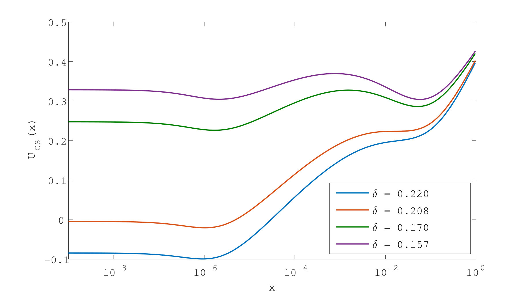 Figure 1
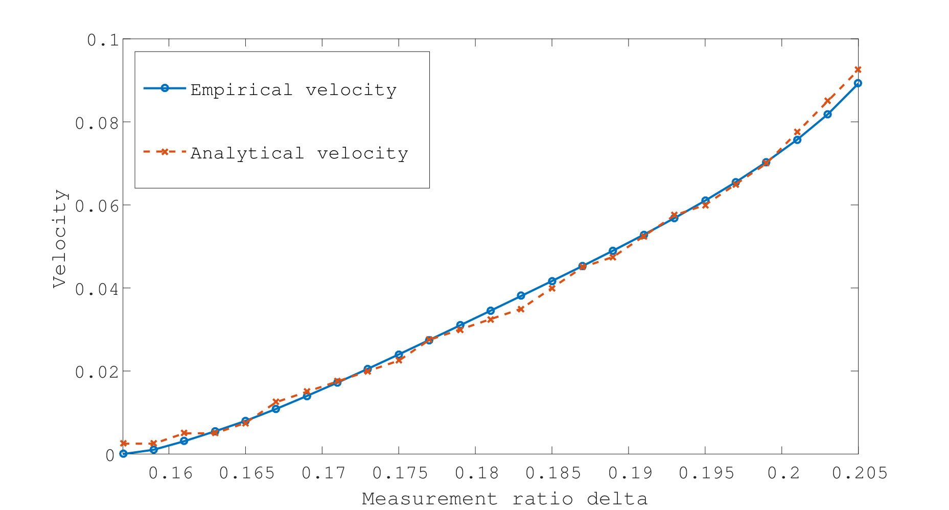 Figure 2
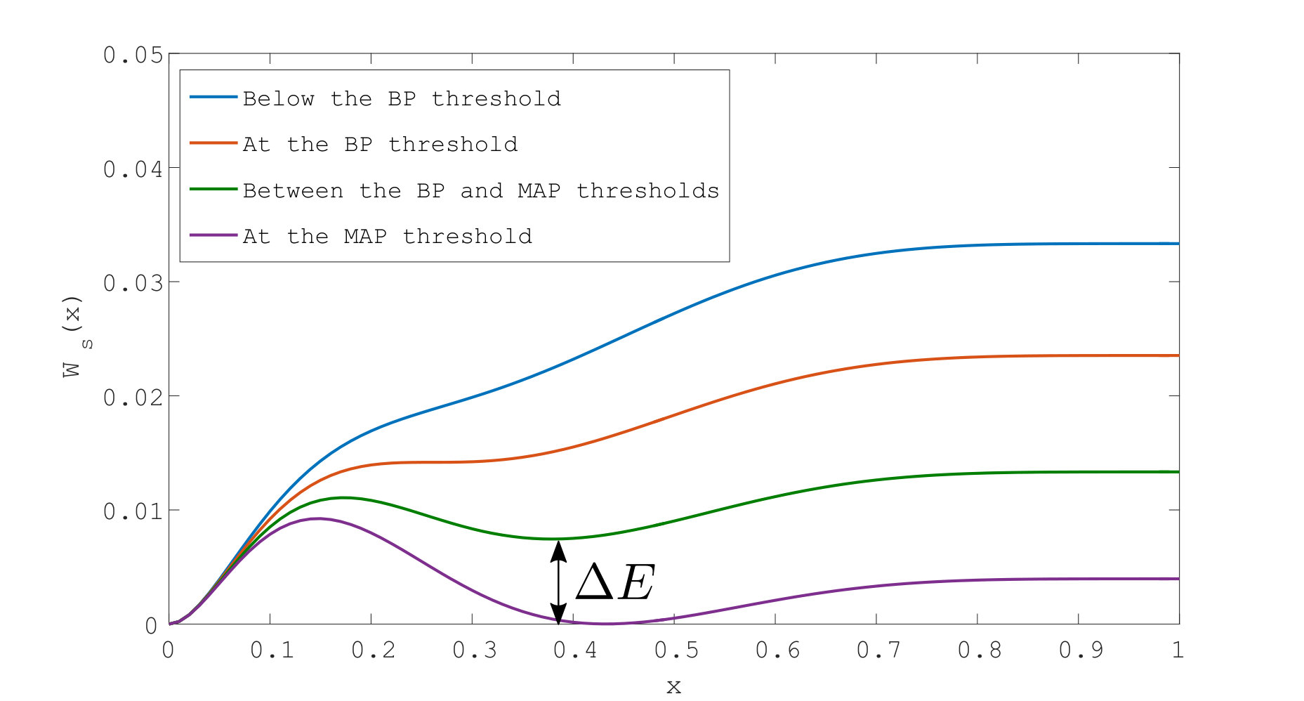 Figure 3
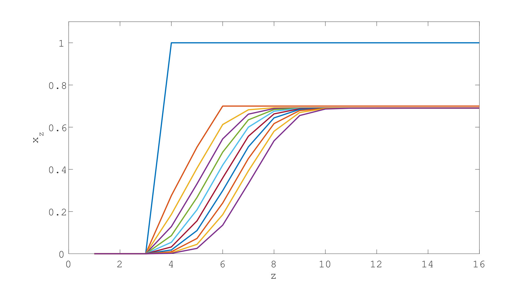 Figure 4
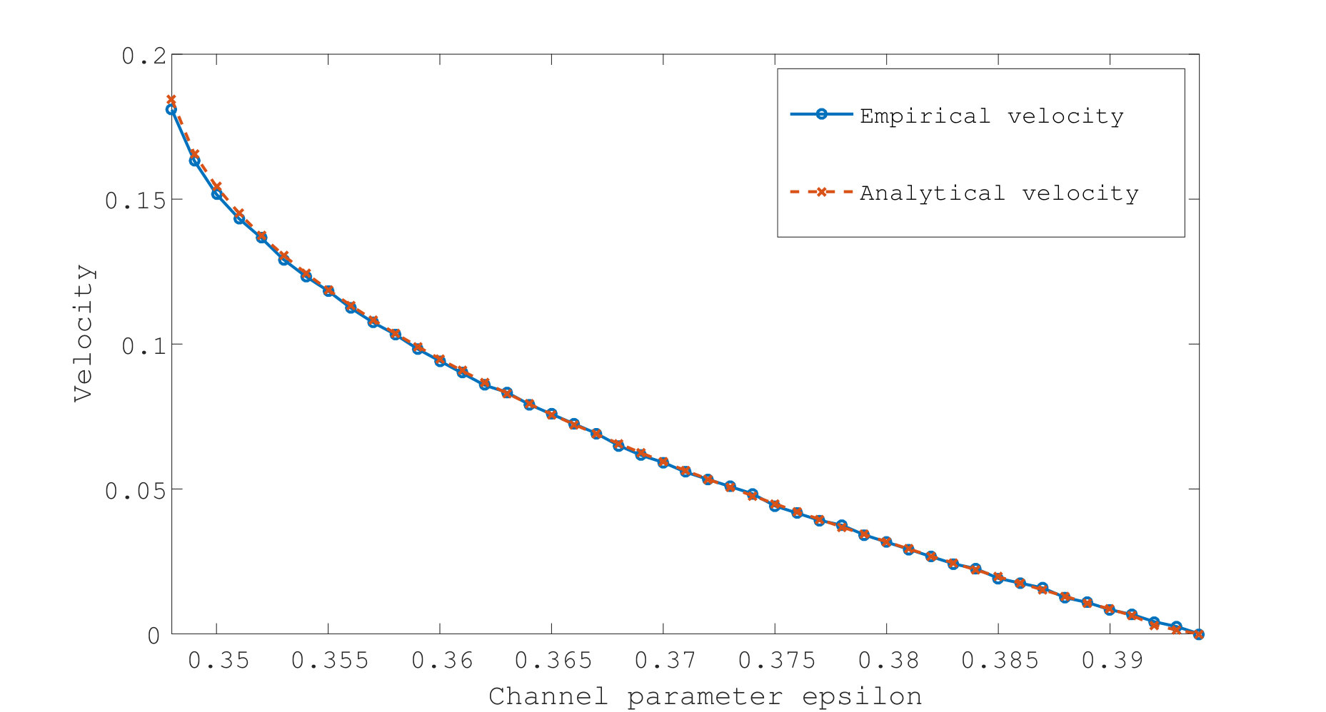 Figure 5
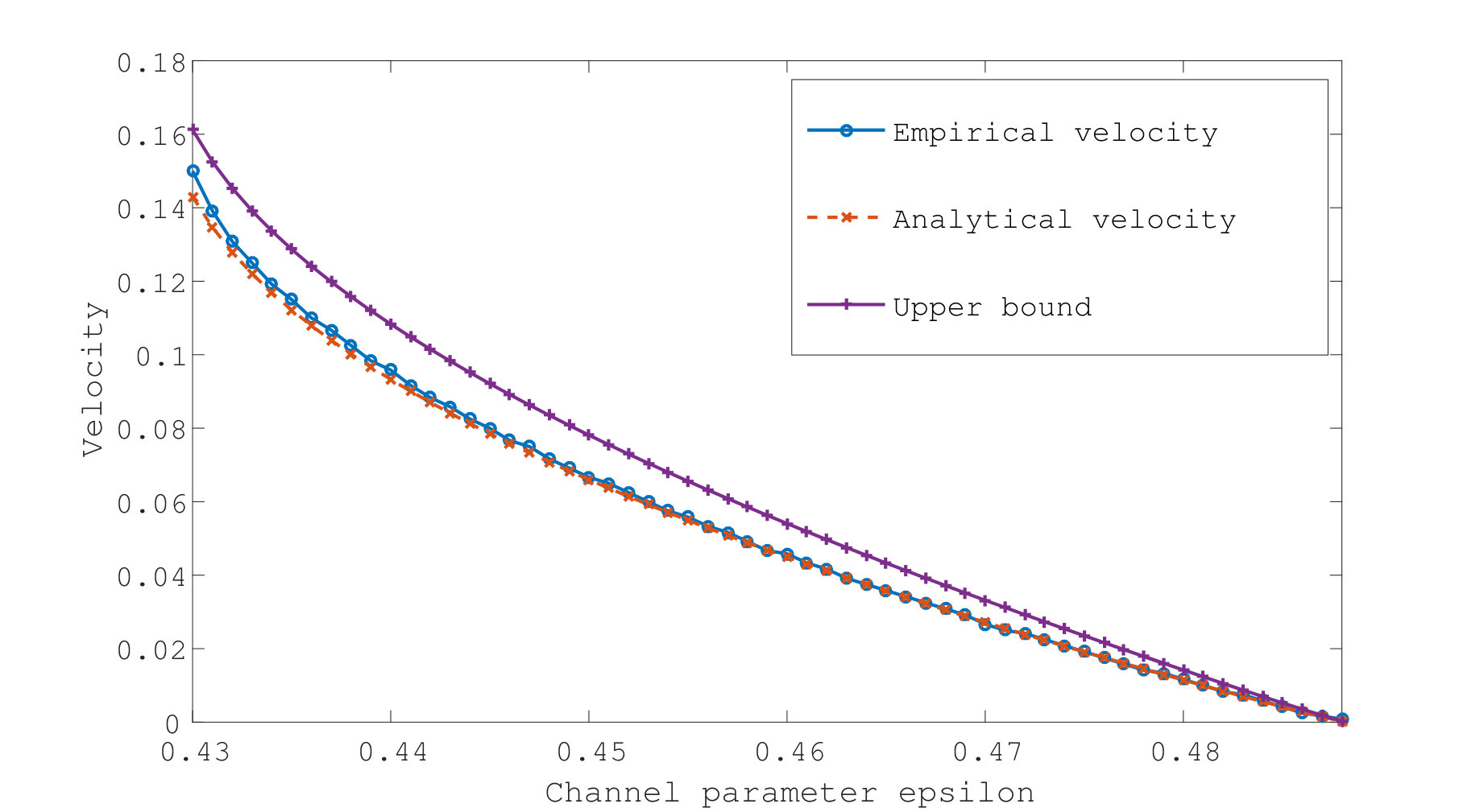 Figure 6
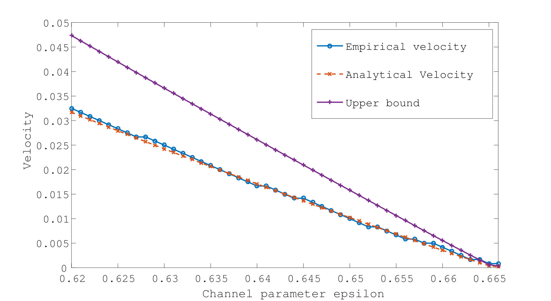 Figure 7
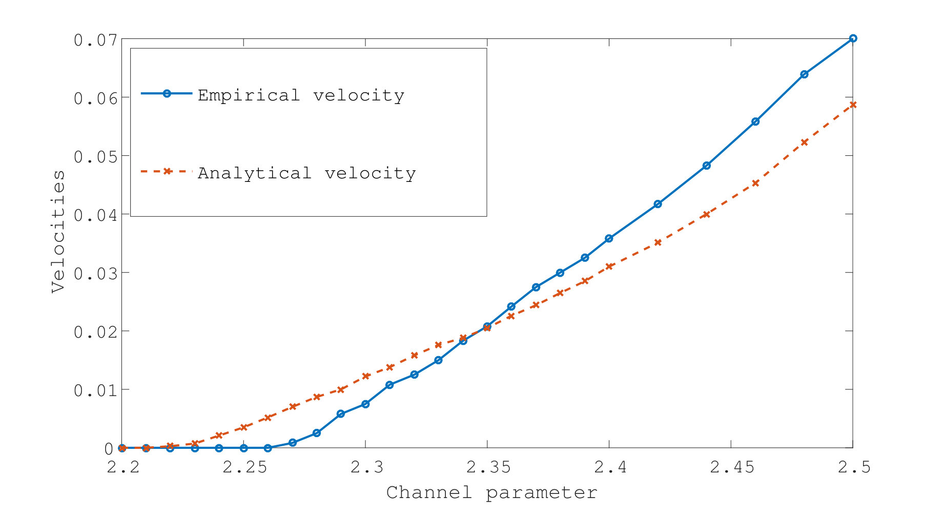 Figure 8
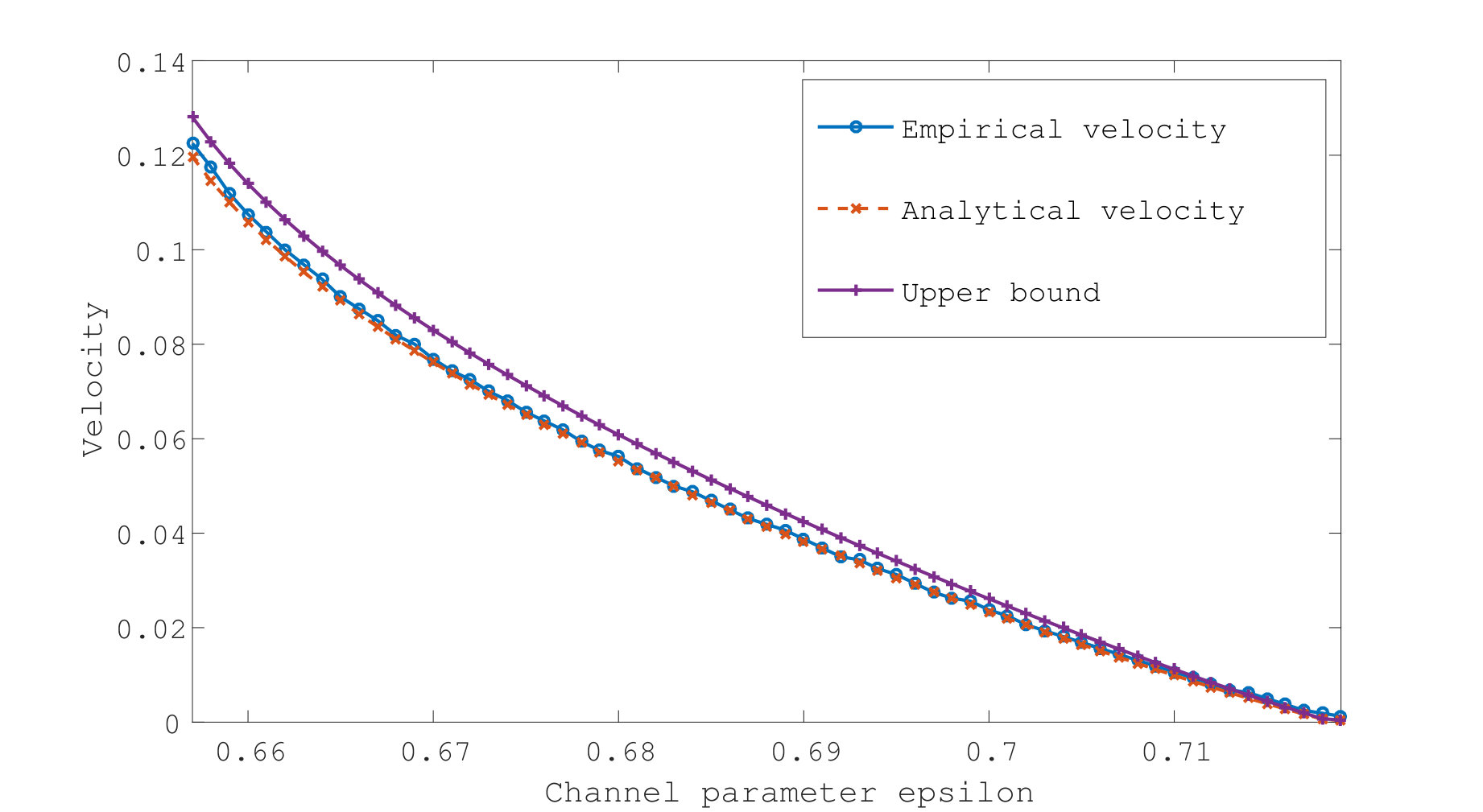 Figure 9
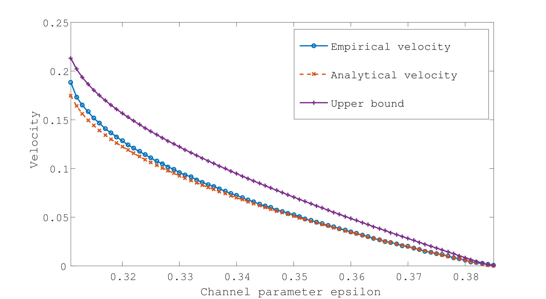 Figure 10
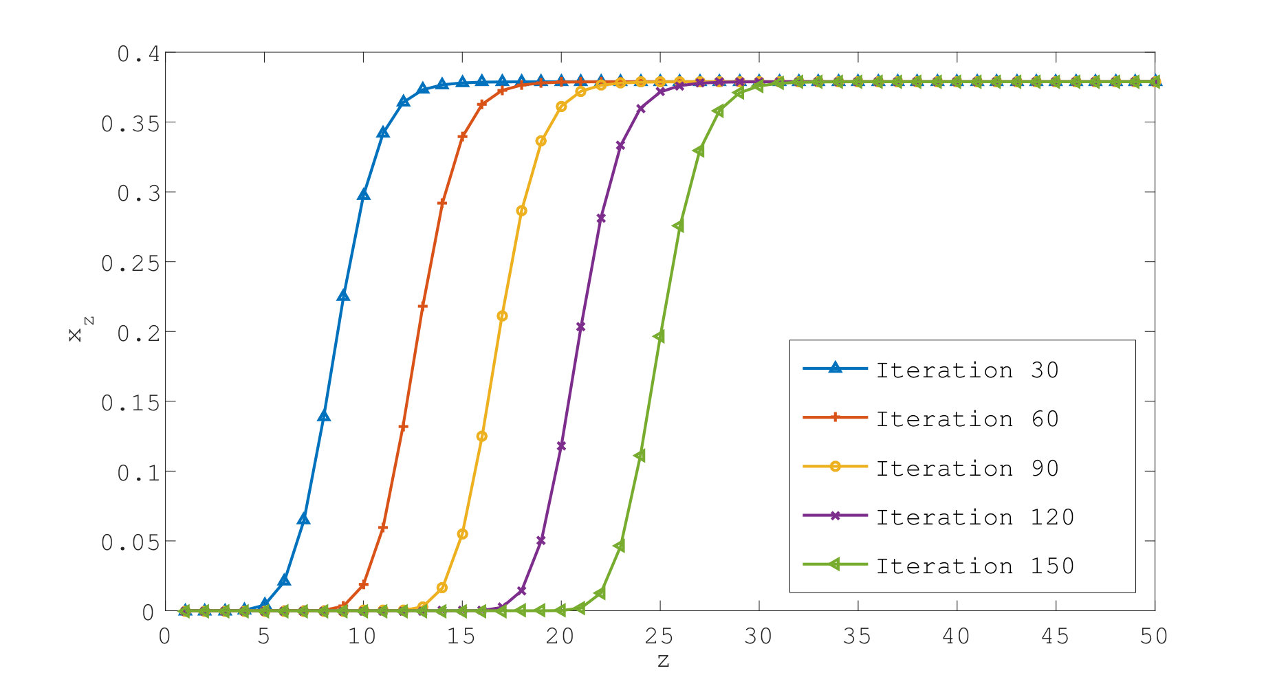 Figure 11
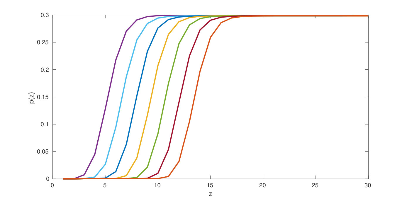 Figure 12
| 0.0325 | 0.0335 | 0.0337 | 0.0339 | |
| 0.0473 | 0.0410 | 0.0380 | 0.0356 |
| 0.0667 | 0.0458 | 0.0267 | 0.0117 | |
| 0.0660 | 0.0449 | 0.0272 | 0.0115 | |
| 0.0506 | 0.0373 | 0.0240 | 0.0108 | |
| 0.0781 | 0.0541 | 0.0332 | 0.0142 | |
| 0.6970 | 0.5008 | 0.3068 | 0.1291 |
| 2.33 | 2.35 | 2.38 | 2.40 | |
| 0.0176 | 0.0205 | 0.0265 | 0.0310 | |
| 0.0150 | 0.0208 | 0.0300 | 0.0358 | |
| 0.0237 | 0.0258 | 0.0312 | 0.0381 | |
| 0.0217 | 0.0250 | 0.0308 | 0.0342 |
| l | r | |||
|---|---|---|---|---|
| 3 | 6 | 0.4881 | 2.155 | 1.960 |
| 4 | 8 | 0.4977 | 2.120 | 1.779 |
| 5 | 10 | 0.4994 | 2.095 | 1.733 |
| 6 | 12 | 0.4999 | 2.075 | 1.722 |
| 4 | 12 | 0.3302 | 2.140 | 1.778 |
| 5 | 15 | 0.3325 | 2.115 | 1.746 |
| 4 | 6 | 0.6656 | 2.100 | 1.735 |
Peer Reviews
No public reviews on file for this paper yet. If you reviewed it on a platform where reviews are public (OpenReview, ICLR, NeurIPS, ICML), you can paste yours below so the community can read it here.
Videos
No videos yet. Explain this paper in a talk, walkthrough, or lecture? Add one.
The Velocity of the Propagating Wave
for Spatially Coupled Systems with
Applications to LDPC Codes
Rafah El-Khatib, and Nicolas Macris R. El-Khatib and Nicolas Macris are with the School of Computer and Communication Sciences, École Polytechnique Fédérale de Lausanne (EPFL), Lausanne, Switzerland, e-mails: {rafah.el-khatib,nicolas.macris}epfl.ch.
Abstract
We consider the dynamics of message passing for spatially coupled codes and, in particular, the set of density evolution equations that tracks the profile of decoding errors along the spatial direction of coupling. It is known that, for suitable boundary conditions and after a transient phase, the error profile exhibits a “solitonic behavior”. Namely, a uniquely-shaped wavelike solution develops, that propagates with constant velocity. Under this assumption we derive an analytical formula for the velocity in the framework of a continuum limit of the spatially coupled system. The general formalism is developed for spatially coupled low-density parity-check codes on general binary memoryless symmetric channels which form the main system of interest in this work. We apply the formula for special channels and illustrate that it matches the direct numerical evaluation of the velocity for a wide range of noise values. A possible application of the velocity formula to the evaluation of finite size scaling law parameters is also discussed. We conduct a similar analysis for general scalar systems and illustrate the findings with applications to compressive sensing and generalized low-density parity-check codes on the binary erasure or binary symmetric channels.
Index Terms:
Message passing, density evolution, potential functional, threshold saturation, soliton, wave propagation, compressive sensing.
I Introduction
Spatial coupling was first introduced by Felstrom and Zigangirov in the context of low-density parity-check (LDPC) codes [1]. Spatially coupled codes have been shown to be capacity-achieving on binary memoryless symmetric (BMS) channels under belief propagation (BP) decoding. The capacity-achieving property is due to the “threshold saturation” of the BP threshold of the coupled system towards the maximum a-posteriori (MAP) threshold of the uncoupled code ensemble [2], [3]. Spatial coupling has also been applied to several other problems besides channel coding [4], [5], such as lossy source compression [6], [7], compressive sensing [8], [9], [10], random constraint satisfaction problems [11], [12], [13], and a coupled Curie-Weiss (toy) model [14], [15].
Consider a single (uncoupled) LDPC code. To construct the corresponding coupled code of spatial length , we take replicas of the single system and “couple” every adjacent single systems by means of a uniform window function. At every iteration of the BP algorithm, the variable and check nodes of the coupled graph exchange messages which are described by a set of coupled density evolution (DE) iterative equations. The solution to the DE equations, called the decoding profile , is a vector of “error distributions” (more precisely, distributions of the BP log-likelihood estimates) along the spatial axis of coupling. More specifically, let the integer denote the position along the spatial direction of the graph construction (on which the replicas are spread). Then the component of , call it , denotes the distribution of the BP log-likelihood estimate at the position. In the special case of the binary erasure channel (BEC) this component is reduced to the usual scalar erasure probability at position along the spatial axis of coupling.
Spatially coupled codes perform well, and are capacity achieving, due to the threshold saturation phenomenon that is proved for general BMS channels in [2], [3]. More specifically, as long as the channel noise is below the MAP threshold, the decoding profile of a spatially coupled code converges to the all- vector after enough iterations of the BP algorithm, where is the Dirac mass at infinite log-likelihood (i.e. perfect knowledge of the bits). In the special case of the BEC, the all- vector corresponds to a vector of scalar erasure probabilities driven to zero by DE iterations. On the other hand, the probability distribution of the log-likelihoods of bits of the corresponding uncoupled code only converge to when the channel noise is below the BP threshold (which is lower than the MAP threshold).
The threshold saturation phenomenon is made possible due to “seeding” at the boundaries of the spatially coupled code. Seeding means that we fix the bits at the boundaries so that the probability distributions of their log-likelihoods are . This facilitates BP decoding near the boundaries, and this effect is propagated along the rest of the coupled chain. The minimum size of the seed that guarantees the propagation of the decoding effect is of the same order as the size of the coupling window; however, an exact determination of the minimum possible such size is an still an interesting open question.
When the channel noise is between the BP and the MAP thresholds, and the underlying uncoupled ensemble has a unique non-trivial stable BP fixed point that blocks decoding, an interesting phenomenon that has been empirically observed is the appearance of a solitonic decoding wave after a certain number of transient iterations of the BP algorithm. This soliton is characterized by a fixed shape that seems independent of the initial condition and has a constant traveling velocity that we henceforth call . This phenomenology is discussed in more details in Section II-C. Figures 2 and 3 in Section II-C show an example of the transient phase and of the soliton in the case of spatially coupled codes on the BEC. The main goal of this work is to derive a formula for the velocity of the soliton for general BMS channels.
The decoding wave has recently been studied in the context of coding when transmission takes place over the BEC. In [16], it is proved that the solitonic wave solution exists and bounds on the velocity of the soliton are derived. However, the independence of the unique shape of the wave from the initial conditions remains an open question. In [17], more complex coupled systems are studied, where it is possible to have more than one non-trivial stable BP fixed point, and there again some bounds on the velocity of the soliton are provided. The solitonic behavior has also been studied for the coupled Curie-Weiss toy model [14] and in [15] a formula for the velocity, as well as an approximation, are derived and tested numerically.
In the first part of this work, we derive a general formula for the velocity of the wave in the asymptotic limit in the context of coding when transmission takes place over general BMS channels (see Equ. (15)). This limit enables us to formulate the problem in a “continuum limit” which makes the derivations quite tractable. We show, with the use of numerical simulations, that this continuum limit yields good approximations for the velocity of the original discrete system. For simplicity, we limit ourselves to the case where the underlying uncoupled LDPC code has only one non-trivial stable BP fixed point.
Our derivation rests on the assumption that the soliton indeed appears. More precisely, we assume that after an initial transient phase, the decoding profile develops a unique shape, independent of the initial condition, and travels with a constant velocity . This assumption can be strictly true only in an asymptotic limit of a very large chain length and a large iteration number (or time). It is an interesting open problem to make this space-time asymptotic limit precise and rigorously prove that the soliton appears and is independent of the initial condition. We conjecture that our velocity formula is exact in such a limit.
The formula for the velocity of the wave greatly simplifies when we consider transmission over the BEC, because the decoding profile reduces to a scalar vector of erasure probabilities. For transmission over general BMS channels, we also simplify the analysis by applying the Gaussian approximation [18], [19]. This consists of approximating the DE densities and the channel by suitable “symmetric” Gaussian densities. Since the mean and the variance of these symmetric Gaussian densities are related by , the analysis then reduces to that of a one-dimensional scalar system, whose technical difficulty is similar to that of the case of transmission over the BEC. We thus obtain a more tractable velocity formula and compare the numerical predictions of these velocity formulas with the empirical value of the velocity for finite values of and . Good agreement is found, on practically the whole range of values within , even for small values of the window size .
It is of theoretical as well as practical interest to have a hold on the analytical expression of the velocity of the wave. The velocity is also related to other fundamental quantities that describe a coding system, such as the finite-size scaling law that predicts the error probability of finite-length spatially coupled codes. In [20], the scaling law for a finite-length spatially coupled code, when transmission takes place over the BEC, is derived. Involved in this scaling law are parameters that can be estimated using the value of the velocity of the decoding wave. Using values of the velocity computed in our work, we provide reasonably good estimates of these parameters.
In the second part of this work, we consider general spatially coupled scalar bipartite systems (that are not restricted to coding) governed by a general message passing algorithm. In this setting, the system is scalar (one-dimensional) since the messages exchanged between the nodes are scalar. Due to seeding at the boundary, the “profile” (we no longer call it the “decoding profile”) exhibits the same phenomenology as in coding. Namely, a solitonic behavior appears after a short transient phase. We derive a formula for the velocity of the soliton for such systems and illustrate it on two applications: compressive sensing and generalized LDPC (GLDPC) codes.
The derivations of the velocity formulas in both parts of the work use the same tools and assumptions. We combine the use of the “potential functional” introduced and used in a series of works [3], [11], [14], [21], [22], as well as the continuum limit which makes the derivations analytically tractable. The potential is a “variational formulation” of the message passing algorithm on coding systems. It is a functional whose stationary points are the fixed points of the density evolution equations described by this algorithm, and has been used to prove threshold saturation in [3] for general BMS channels. A significant part of the formalism in [3] is used in the present work. We also note that potential formulations have been used to characterize the fixed point(s) of general scalar systems at the MAP threshold using displacement convexity in [23], [24]. An extension of the ideas in these works could shed some light on the question of the independence of the soliton’s shape from the initial conditions.
Section II introduces a few preliminary notions that we will need and reviews the phenomenology of the solitonic wave. In Section III, we formulate the continuum limit and state our main formula for the velocity of the soliton on general BMS channels; the derivation is presented in Section IV. Comparisons with numerical experiments are presented in Section V. These concern transmission over the BEC as well as general BMS channels in the so-called Gaussian approximation. We also discuss a possible application of our formula to scaling laws for finite-size ensembles in Section VI. The case of general scalar spatially coupled systems is treated in Section VII, and illustrated for the examples of generalized LDPC codes (on the BEC or BSC channels) and compressive sensing. We present concluding remarks and propose further directions in Section VIII.
A summary of this work has appeared in [25], [26].
II Preliminaries
We consider (almost) the same setting as in [3] and adopt most of the notation introduced in that work. For more information about the formalism in these preliminaries, one can consult [27].
We denote by the space of probability measures on the extended real numbers . Here should be interpreted as a “log-likelihood variable”. We call the measure symmetric if for all measurable sets .
We define an entropy functional that maps a finite probability measure from to a real number. It is defined as
[TABLE]
Note that this is a linear functional. Linearity is used in an important way to compute the entropy of convex combinations of measures (which also yield probability measures). But we will also compute the “entropy” associated to differences of measures by setting . In other words, the entropy functional is extended in an obvious way to the space of signed measures.
In the remainder of this work, we will use the Dirac masses and at zero and infinite log-likelihood, that have entropies and , respectively.
We will also use the standard variable-node and check-node convolution operators and for log-likelihood ratio message distributions involved in DE equations [27]. For , , the usual convolution is the density of
[TABLE]
and is the density of
[TABLE]
More formally, for any measurable set , the operators are defined by
[TABLE]
We note that the identities of the and operators are and , and their annihilators are and . More explicitly,
[TABLE]
Each operation, taken separately, is associative, commutative, and linear. However, when they are taken together, there is no distributive law; also, they don’t associate in the sense that and . We will also use the so-called duality rules
[TABLE]
where and , are differences of probability measures , , , .
II-A Single System
Consider an (uncoupled) LDPC() code ensemble and transmission over the BMS channel. Here, and are the usual edge-perspective variable-node and check-node degree distributions, respectively. The node-perspective degree distributions and are defined by and , respectively. Moreover, consider communication over a family of BMS channels whose distribution in the log-likelihood domain is parametrized by the channel entropy111In the literature, this quantity is often denoted by . .
Let denote the variable-node output distribution of the BP algorithm at iteration . We can track the average behavior of the BP decoder by means of the DE iterative equations that are written as a recursion in terms of the variable-node output distribution as follows
[TABLE]
with initial condition (equivalently, we can take the perhaps more natural initial condition ).
There are two thresholds of interest for us. The first one is the algorithmic threshold; it is defined for a family of BMS channels whose channel distributions are ordered by degradation and parametrized by their entropy . It is also called the BP threshold of the family and is defined as
[TABLE]
The second threshold corresponds to optimal (MAP) decoding
[TABLE]
where is the conditional Shannon entropy of the input given by the channel observations, and is the expectation over the code ensemble.
The potential functional , , of the “single” or uncoupled system is
[TABLE]
The fixed point form of the DE equation (5) is obtained by setting to zero the functional derivative of with respect to . In other words, is equivalent to
[TABLE]
where is a difference of two probability measures (see [3] for the proof of this statement). The BP and MAP thresholds, and , respectively, can be obtained from the analysis of the stationary points of the potential function. See [3], [28] for more details and a rigorous discussion of this issue.
Remark about notation. In the remainder of this work, most of the time, we omit the subscript from and the argument from . This is because we will need a subscript (resp. an argument) that represents the position along the chain in the discrete (resp. continuous) case.
II-B Spatially Coupled System
For standard LDPC codes, the BP threshold is, in general, lower than the MAP threshold . The definitions of the BP and MAP thresholds above extend to the spatially coupled setting. Spatial coupling exhibits two attractive properties. First, the MAP threshold is conserved under coupling in the limit and for all . The proof of this statement is found in [28] (see also [29], [30]). Second, the BP threshold of the coupled system saturates to its MAP threshold as proved in [2], [3]. The main consequence of threshold saturation is that one can decode perfectly up to the .
Let us now describe the density evolution and potential functional formalism for the spatially coupled code ensemble. Consider “replicas” of the single system described in Section II-A, placed on the spatial coordinates . The system at position is coupled to neighboring systems by means of a coupling window. For simplicity, we consider a uniform coupling window. We denote by the variable-node output distribution at position on the spatial axis and at time . The DE equation of the coupled system takes the form
[TABLE]
In this equation, , for and for . Furthermore, we fix the left boundary to for , for all . These conditions express perfect information at the left boundary which is what enables seeding and the decoding wave propagation along the chain of coupled codes. The initial condition (8) is for .
It will be convenient to work with a smoothed version of the profile , namely , which is the check-node input distribution. Then, using this change of variables, (8) can be rewritten as
[TABLE]
Just as in the single system case, this DE equation can be expressed as the stationarity condition of a potential functional (see [3])
[TABLE]
where . The fixed point form of (9) is equivalent to for where are differences of probability measures.
II-C Phenomenological observations
Our derivation is far from rigorous and is based on an assumption derived from a phenomenological picture observed from simulations. We summarize the main observations in this paragraph for the case of transmission over the BEC channel. This channel also gives us the opportunity to illustrate the formalism outlined in Sections II-A and II-B in a concrete case.
The BEC has channel distribution , where is the erasure probability, and (hence ). The density of the BP estimates of log-likelihood variables can be parametrized as , where is interpreted as the erasure probability at iteration . The DE equation becomes a one-dimensional iterative map
[TABLE]
over scalars in . These iterations are always initialized with or, equivalently, . The corresponding fixed point equation is the stationarity condition for the potential function
[TABLE]
Note that the potential function is defined up to a constant which is set here so that . Figure 1 illustrates the potential function for a -regular Gallager ensemble, for several values of . For , the potential function (12) is strictly increasing, and equivalently the DE iterations are driven to the unique minimum at . At a horizontal inflexion point appears and a second non-trivial local minimum appears; this minimum corresponds to the non-trivial fixed point reached by DE iterations. It is known that the MAP threshold is equal to the erasure probability where the non-trivial local minimum is at the same height as the trivial one and that decoding becomes impossible once the non-trivial minimum becomes a global minimum. For this example, this happens when . Figure 1 also shows the energy gap that is defined for as . At the MAP threshold, we have .
Let us now describe the phenomenology of the soliton (decoding wave) for spatially coupled codes. Our discussion is limited to the case where the underlying code ensemble has a single non-trivial DE fixed point (equivalently, the potential function has a single non-trivial local minimum). One can show that this is always the case for regular code ensembles. For irregular degree distributions the situation may be more complicated with many non-trivial fixed points that appear. For transmission over the BEC, equation (9) reads
[TABLE]
Here, for and for . Furthermore, we fix the left boundary to for , for all . These are the “perfect seeding” conditions which enable the initiation of decoding. The initial condition for the iterations is (or ) for .
The evolution of the decoding wave can be decomposed into two phases: a transient and a stationary phase. In the transient phase, we observe a profile of erasure probabilities changing shape. The segment initialized to quickly drops to where it remains stuck on the far right for large values of . The seeding region, on the other hand, starts progressing towards the right-hand side and, after a few iterations, a fixed profile shape develops. This transient phase is illustrated in Figure 2 for an irregular code. Overall, it only lasts for a few iterations (of the order of iterations in this example). After this transient phase is over, one observes a stationary phase with a solitonic behavior, as depicted in Figure 3. The profile of erasure probabilities has a stationary shape with a front at position that moves, at a constant speed, towards the right. The soliton is relatively well-localized within approximately positions and quickly approaches for and for . The stationary phase and its soliton are depicted in Figure 3 for a finite spatially coupled -regular ensemble with chain length and for . In this figure, we plot the decoding profile every 30 iterations starting at the iteration (the leftmost curve) and until the iteration (the rightmost curve). The kink increases sharply from to over a width of the order of .
III Continuum limit and main result
III-A Continuum Limit
We now consider the coupled system in the continuum limit, in which the length of the coupling chain is first taken very large , and then the window size is taken very large . The continuum limit has already been considered for the special case of the BEC in [16], [23], [24]. We slightly abuse notation by keeping the same symbols for the profile, the spatial position, and the channel distribution in the continuum limit. Thus, we denote by the continuous profile of distributions and set . We then replace so that the new is the continuous variable on the spatial axis, .
In view of the discussion of the phenomenology in Section II-C, we consider the class of profiles satisfying the “natural boundary conditions” when for all , when for all , where is the unique non-trivial stable fixed point of DE for the single system Equ. (5).
The BMS channel distribution is now also continuous, and we denote by the channel distribution at the continuous spatial position . The DE equation (9) then takes the form
[TABLE]
The initial condition at is given by a profile that interpolates between the two limiting values of the boundary condition, namely when and when .
III-B Statement of Main Result
We consider the channel entropy . The phenomenology tells us that: (i) after a transient phase, the profile develops a fixed shape ; (ii) the shape is independent of the initial condition; (iii) the shape travels at constant speed ; (iv) the shape satisfies the boundary conditions for and for . We thus formalize these observations and make an ansatz:
Ansatz. For each there exist a constant and a family of probability measures (indexed by ) satisfying the boundary conditions for and for , such that, for and , the solution of DE (14) is independent of the initial condition and satisfies .
Implicit in this ansatz is that we restrict ourselves here to underlying code ensembles that have only one non-trivial (stable) BP fixed point. This is true for regular codes for example (but is not limited to this case). Ensembles with many non-trivial fixed points could lead to more complicated phenomenologies as emphasized in [17] and would require to modify the ansatz.
Velocity of the soliton for general BMS channels. Under the assumption above the velocity of the soliton is given by
[TABLE]
where is the energy gap defined as
[TABLE]
and we recall that is the potential (6) of the uncoupled system , is the non-trivial BP fixed point to which the uncoupled system converges, and is the trivial fixed point (Dirac mass at infinity).
Let us make a few remarks. In this formula, the prime denotes the derivative which is to be interpreted as a difference between two measures. The energy gap is only defined for , that is, when the single potential has a non-trivial non-negative local minimum (see e.g. Figure 1). It is exactly equal to zero when , which confirms the fact that the velocity of decoding is zero (no decoding occurs) in this case. Note also that, with our normalizations, .
Formula (15) involves the shape . Using the DE equation, the ansatz , and the approximation , valid for small , we find after a change of variables that is the solution of
[TABLE]
To obtain the shape and the velocity , one must iteratively solve the closed system of equations formed by (15) and (17). Note that the assumption of small used above is strictly valid for close to . However, numerical simulations confirm that in practice the resulting velocity formula is precise over the whole range .
IV Derivation of velocity formula for BMS channels
Let us briefly outline of the main steps of derivation. We first write down a potential functional which gives, in the continuous setting, the DE fixed point equation corresponding to (14). This enables us to formulate the DE iterations as a sort of gradient descent equation (Section IV-A). From there on, we use the ansatz in Section III-B to derive the velocity formula (15).
IV-A Density evolution as gradient descent
We call the potential functional of the coupled system in the continuum limit obtained from (10). This limit involves an integral over the spatial direction and, in order to get a convergent result, we must subtract a “reference energy”. Essentially, any static reference profile, here called , that satisfies the boundary conditions , and , , will do the job. For concreteness, one can take a Heaviside-like profile , , , . The potential functional is thus defined as follows,
[TABLE]
where is a -dependent functional of equal to
[TABLE]
In Appendix A, we calculate the functional derivative of in a direction defined as
[TABLE]
and find
[TABLE]
From (14) and (21) we deduce that
[TABLE]
We note that, using the duality rule (4) for and (recall that must be a difference of two measures so that also is such a difference) and the associativity of , this equation can also be formulated as
[TABLE]
In this form, we recognize a sort of infinite-dimensional gradient descent equation in a space of measures. This reformulation of DE forms the basis of the derivation of the velocity formula.
IV-B Final steps of the derivation
The potential functional can be decomposed in a “single system” part and a contribution that contains the “interaction” due to coupling. We have
[TABLE]
with
[TABLE]
where
[TABLE]
and
[TABLE]
Note, for future use, that in fact is the single system potential (6) “at position ”. With these definitions, the gradient descent equation (23) can be written as
[TABLE]
Now, we use the ansatz to compute the three terms in this equation in the regime , such that . We will choose the direction .
We start with the left-hand side of (29). From and the approximation , together with the special choice of , we can rewrite the left hand side of (29) as
[TABLE]
Using the commutativity of the operator , this is equal to
[TABLE]
Note that we can shift the argument in the integrals , and this term becomes independent of time.
Now, we consider the first functional derivative on the right hand side of (29), when . It should be clear that we can immediately make the change of variables in the integrals which simplifies the formulas. By the calculations in Appendix A, we find
[TABLE]
In order to simplify the above, we remark the following
[TABLE]
Noticing that the first two terms on the right-hand side cancel out, and using the duality rule (4) for the third term, we get the integrand in (32). In other words, the integrand in (32) equals and
[TABLE]
We now show that the functional derivative of the interaction part in (29) does not contribute when is replaced by . By directly applying the definition of the functional derivative, we find
[TABLE]
We notice that the integrand is a total derivative; namely, it is equal to
[TABLE]
Due to the boundary conditions, we have and , and we can conclude that the total derivative integrates to zero, thus
[TABLE]
Finally, replacing (31), (33), and (35) in (29) we get the simple relationship
[TABLE]
which yields the velocity formula (15).
V Applications to specific channels and comparisons with Numerical Experiments
V-A Binary Erasure Channel (BEC)
The formula for the velocity, when transmission takes place over the BEC, can be obtained by directly simplifying the general formula in (15). We note that, since the BEC yields a scalar system, one can also use the formula for general scalar systems in Section VII (that covers cases beyond coding theory also). We will suppose that the underlying code LDPC is such that the DE equation has a single non-trivial fixed point . Furthermore, we fix (recall the channel entropy reduces to here).
The channel distribution can be written as , and the profile is of the form where is the scalar erasure probability at position and time . This tends to a fixed shape
[TABLE]
where satisfies , . We have also
[TABLE]
We also note the following identities valid for scalar maps (such as , , , and their derivatives)
[TABLE]
Let us compute the denominator of (15). Using (3), (38), and (39) we have
[TABLE]
and since , , and the entropy functional is linear, we obtain the denominator of (15) as
[TABLE]
For the numerator of (15), we have , where the single system potential on the BEC is obtained from (6) using again (3) and (39). The exercise yields
[TABLE]
Putting together these results, the velocity (15) becomes
[TABLE]
(Note that, with our normalizations, for all .) The erasure profile has to be computed from the one-dimensional integral equation
[TABLE]
Obviously, the velocity vanishes when since then . An important quantity is the slope of the velocity at . To compute it, we remark that has an explicit dependence on , as well as an implicit one through . Thus,
[TABLE]
so that, for , the Taylor expansion to first order yields
[TABLE]
Note that we used where is defined as the point where the potential is stationary and vanishes. This yields the linear approximation for the velocity
[TABLE]
where is the erasure probability profile obtained when .
It is interesting to compare (40) with the upper bound of Theorem 1 in [17] for a discrete system
[TABLE]
In [17] the derivation of the bound yields (for and large enough) but it is conjectured based on numerical simulations that would be a tight bound. Obviously, (40) and (43) are consistent. We note for reference that another upper bound is also derived in [17], namely
[TABLE]
where and and are respectively the non-trivial unstable and stable fixed points of the potential of the uncoupled system . We do not discuss this further because in practice this turns out to be a very loose bound.
We now compare the analytical velocity formula (40) with the empirical velocity (called below) obtained by simulating the discrete DE equation; we show that it provides a very good approximation for the (real) value of the velocity even for relatively small values of . For the simulations, we consider the spatially coupled and -regular code ensembles, as well as two irregular LDPC codes (described later). We run the simulations for several values of the chain length and the window size . The empirical velocity is the velocity calculated from erasure probability profiles of the discrete DE equation. Consider two (discrete) profiles and at any two iterations and , respectively, with . After the transient phase is over, the profiles are identical up to translation. We call a “kink” the part of the profile where there is a fast increase from [math] to in the erasure probability. The kink “position” is the coordinate such that the height is equal to , and is the difference of two such positions (on two different profiles). Then, the empirical velocity is
[TABLE]
In practice, we get reliable results by taking pairs of profiles separated by iterations and averaging this ratio over every consecutive pair of profiles. Note that we normalize the velocity by to be able to compare systems with different window widths.
In Table I, we give empirical values of the normalized velocities for the spatially coupled -regular code ensemble, with transmission over the BEC(0.6), when the spatial length is positions and the channel parameter is fixed to (between the BP and MAP thresholds), for different values of the window size . We observe that the result of our formula gives a good estimate of the empirical velocity for all the demonstrated values of the window size. We also observe that the linear approximation gives a good estimate when the channel parameter is not too far from the MAP threshold . The upper bound [17] gives a better estimate as the window size grows larger.
In Table II, we give empirical values of the normalized velocities for the spatially coupled -regular code ensemble, with transmission over the BEC(), when the spatial length equals and the window size , for different values of the channel parameter . One can compare these values with those in [17] (up to a factor equal to due to the normalization). The result of the formula gives the closest estimate to the empirical velocity for all values of .
Figures 4 and 5 show the empirical velocity , the analytical velocity , and the upper bound for the spatially coupled -regular code ensemble, with spatial length and window size . We remark that our formula fits very well, for the -regular code, with the empirical velocity for all values of the channel parameter . The agreement is quite good also for the -regular code and very good for more than half of the interval .
We also illustrate the results for two irregular code ensembles in Figures 6 and 7. The first one has node degree distributions and , spatial length , and window size . The agreement between and is excellent for the whole range . The second one has and , spatial length , and window size . The agreement between the velocities is also very good for most of the range .
V-B Gaussian Approximation (GA)
DE equations relate probability densities and as such we may need to track an infinite set of parameters (except for the BEC where the space of densities can be parametrized by a single real number). In many situations, such as the case when we have large degrees, for example, the densities are well approximated by Gaussians, which enables us to project the DE equations down to a low dimensional space. There are several variants of the Gaussian approximation (see for example [31], [18], [19]), and here we use it in a form called the “reciprocal channel approximation” proposed in [18], [19].
The idea is to assume that the densities of the LLR messages appearing in the DE equations are symmetric Gaussian densities. Such densities take the form
[TABLE]
with the mean and variance satisfying . Furthermore, the channel density is replaced by that corresponding to a BIAWGNC() with the same entropy . Density evolution can then conveniently be expressed in terms of the entropies . This is done as follows. Let denote the entropy222For indications on the numerical implementation of this function see [27], pp.194 and 237. of a symmetric Gaussian density of mean given by
[TABLE]
Thus denotes the mean of a symmetric Gaussian density of entropy . Take two symmetric Gaussian densities and of means and and entropies and . We have, in general,
[TABLE]
which just expresses the fact that a usual convolution of two Gaussian densities of means and is a Gaussian density of mean . On the other hand is not exactly Gaussian so there is no exact formula but the idea here is to preserve the duality rule . Writing this relation as
[TABLE]
and noting that , suggests the approximation
[TABLE]
Looking at the entropies of the DE equations (47) and (48) imply (we will limit ourselves to regular codes for simplicity)
[TABLE]
and setting , we find
[TABLE]
These equations can be combined into
[TABLE]
The corresponding potential function is easily found from (6)
[TABLE]
For the coupled system, we denote by the average over positions of the entropy of symmetric Gaussian densities emanating from the variable nodes. The coupled DE equations then take the form
[TABLE]
This coupled recursion can be solved with appropriate boundary conditions and one observes a scalar wave propagation, as shown in Figure 8.
We are now ready to discuss the application to the velocity formula. The continuum limit is obtained exactly as in Section III-A. The assumption that the density tends to a fixed shape after the transient phase implies that its entropy tends to , where is a scalar function (independent of initial conditions) satisfying the integral equation
[TABLE]
and the boundary conditions and where is the non-trivial fixed point of (51). We will now show that the velocity formula reduces to
[TABLE]
To derive (55), we consider the denominator in (15) and write it as follows
[TABLE]
Computing each entropy in the Gaussian approximation, we find for the bracket on the right-hand side
[TABLE]
In Appendix B, we compute the limit of this term when by appropriate Taylor expansions and find
[TABLE]
This concludes the derivation of (55).
Table III gives a comparison of analytical and empirical velocities, and , obtained for the and the -regular ensembles, for a spatial length of and a window size for different values of (twice the signal to noise ratio). We also plot both velocities for the -regular ensemble for the same parameters in Figure 9. We conjecture that the errors incurred from these plots are due to numerical errors involved in computing the functions and its inverse.
VI Application to Scaling Laws for Finite-Length Coupled Codes
The authors in [20] propose a scaling law to predict the error probability of a finite-length spatially coupled code when transmission takes place over the BEC. The derived scaling law depends on scaling parameters, one of which we will relate to the velocity of the decoding wave. The ensemble considered in [20] differs slightly from the purely random ensemble we consider in this work. However, as we will see, our formula for the velocity yields results that are reasonably good for this application. We briefly describe this ensemble and the scaling law.
The ensemble combines the benefits of purely random codes (that we consider in this work) and protograph-based codes [32]. The randomness involved in the construction makes the ensemble relatively easy to analyze, and the structure added to the construction due to its similarity to protograph-based codes improves the performance of the code. The ensemble is constructed as follows: Make copies of an uncoupled code at positions . All edges are erased then reconnected such that a variable node at position has exactly one edge with each set of check nodes at positions , where . The check nodes are chosen such that the regularity of their degree is maintained. Therefore, every variable node has emanating edges and every check node has such edges.
We consider transmission over the BEC. In this case, the BP decoder can be seen as a peeling decoder [33]. Whenever a variable node is decoded, it is removed from the graph along with its edges. One way to track this peeling process is to analyze the evolution of the degree distribution of the residual graph across iterations, which serves as a sufficient statistic. This statistic can be described by a system of differential equations, whose solution determines the mean and variance of the fraction of degree-one check nodes and the variance around this mean at any time during the decoding process. We call the mean.
It has been shown in [20] that there exists a steady state phase where the mean and the variance are constant. It is exactly during this phase that one can observe the progression of the soliton. We note that here we consider one-sided termination instead of two-sided termination (as considered in [20]), so the fraction here is equal to half the fraction called in [20].
Let denote the BP threshold of the finite-size ensemble (for large this is close to due to threshold saturation). We can write the first-order Taylor expansion of \hat{r}_{1}\big{|}_{\epsilon} around as
[TABLE]
where . Thus, for a given and since \hat{r}_{1}\big{|}_{\epsilon_{(\ell,r,L_{c})}}=0 (by definition), we obtain
[TABLE]
This parameter enters in the scaling law and is therefore quite important. So far, it has been determined only experimentally. It would clearly be desirable to have a theoretical handle on . It is argued in [20] that where and is a real positive constant that behaves like , i.e.,
[TABLE]
It is expected that this formula becomes exact in an asymptotic limit where threshold saturation takes place . Using the linearization (42), we obtain
[TABLE]
The parameter is simply equal to the erasure probability times the slope of the velocity at .
We compare the values of and for different values of and , at a channel parameter , in Table IV. The experimental values of are taken from [20] and, for those of , we use the analytical velocity (40). We observe that the numbers roughly agree. There are two reasons that can explain the discrepancies. Firstly, we derive the velocity for the purely random spatially coupled graph ensemble whereas the ensemble considered in [20] is more structured. Note also that as , increase, the window size of the structured ensemble increases, so the finite size effects at fixed may be more marked. Secondly, expression (59) is valid when , whereas in IV , which is relatively large (this choice in [20] is due to stability issues in numerical integration techniques when ). We conjecture that the second issue is the dominant reason for the difference between the values of and and that, in fact, the velocity for the structured ensemble is not very different from the one predicted by our formula (40).
VII Velocity for General Scalar Coupled Systems
In this section, we consider general scalar spatially coupled systems. That is, we do not restrict ourselves to coding problems; however, we only consider systems in which the “density evolution type” analysis of message passing algorithms involves scalar values. Our main result is again a general formula for the velocity of the soliton in the framework of general scalar coupled systems. There are numerous systems that fall in this class - coding with transmission on the BEC being one of the simplest - and in Sections VII-D, VII-E we will illustrate our results with two examples, namely generalized LDPC codes on the BEC and BSC, as well as compressive sensing.
VII-A General scalar systems
We adopt the framework and notation in [21]. We denote by where the interval of values for the control parameter . Consider bounded, smooth functions that are increasing in both their arguments and where , and . The scalar recursions that interest us are
[TABLE]
where is the iteration number. The recursion is initialized with . Since , the initialization of (61) implies that and more generally . Thus will converge to a limiting value and this limit is a fixed point since and are continuous. The fixed points of the recursion (61) can be described as stationary points of a single system potential function defined as
[TABLE]
where and . Without loss of generality, this function is normalized so that .
We define as the fixed point of the recursion (61) that is reached with an initialization . Furthermore, the algorithmic threshold333Here, we mean the algorithmic threshold of the message passing algorithm underlying the recursion. is defined as
[TABLE]
The monotonicity of and implies that, for , the basin of attraction of is the whole interval . Moreover is the unique stationary point of the potential function and is a minimum since it is an attractive fixed point. For we have and we set (where depends on ). Note that this is an attractive fixed point and is thus a (local) minimum of . The two attractive fixed points are separated by at least one unstable fixed point which is a local maximum of . We henceforth assume that there does not appear any other fixed point besides , , and . With this assumption in mind, we define the energy gap as
[TABLE]
and the potential threshold as the unique value such that (it can be shown that in non-increasing in ).
The corresponding spatially coupled recursions are obtained by placing replicas of the single system on the spatial positions and coupling them with a uniform coupling window of size . The coupled recursion takes the form
[TABLE]
Motivated by the phenomenology observed in many examples (e.g. for the BEC or for compressve sensing), in order to study the stationary phase where a soliton appears, we fix the boundary conditions as , for and all . The initialization of the recursion is , for . The corresponding potential functional is given by
[TABLE]
where . The fixed point equation (65) can be obtained by setting the derivative with respect to of the potential to zero.
The spatially coupled recursions (65) display the threshold saturation property. Namely, for all the fixed point , , of the recursion (65) is equal to a constant profile . In the remainder of this section, we consider the range . It is for these values of the parameter that a soliton propagating at finite speed is observed, after a transient phase lasting only for a few iterations. The soliton is a kink with a front at position , making a quick transition of width , between the two values for and for .
The simplest example to keep in mind for the setting described above, as well as for the next paragraph, is the case of LDPC codes with transmission over the BEC where and and is equal to (12). Here , , and is the non-trivial BP fixed point.
VII-B Continuum limit and velocity formula for scalar systems
We consider the system in the limit and formulate a continuum approximation. The coupled recursion (65) becomes
[TABLE]
We take the boundary condition when and when . This boundary condition captures the profiles obtained after the transient phase has passed, and is well adapted to the study of the soliton propagation.
Velocity formula for scalar systems. As before, we assume that there exists a constant such that, for and , the profile , where is independent of the initial condition and satisfies , . Under this assumption, the velocity of the soliton is
[TABLE]
where the shape satisfies
[TABLE]
VII-C Derivation of the velocity formula (68)
The derivation of (68) follows closely that in Section IV-B, so we will be quite brief. The first step is to introduce a continuum version of , which we call . We define as a static (time-independent) profile that satisfies the boundary conditions when and when (for example, one may take a Heaviside step function). This is a reference profile in order to have well-defined integrals in the following expression
[TABLE]
As long as and converge to their limiting values fast enough, the integrals over the spatial axis are well defined. Evaluating the functional derivative444Defined as of in an arbitrary direction , we find that (67) is equivalent to a gradient descent equation
[TABLE]
Now we use the ansatz and apply (70) for the special direction . Using also the approximation for small we get (after a change of variables )
[TABLE]
We then proceed to compute the right-hand side of (70). We split the potential functional into two parts: the “single system potential” that remains if we ignore the coupling effect, and the “interaction potential” that captures the effect of coupling. That is, , with
[TABLE]
The computation of each functional derivative at in the direction yields
[TABLE]
and
[TABLE]
Replacing (72) and (73) in (70), we obtain the velocity formula (68).
VII-D Generalized LDPC (GLDPC) Codes
A GLDPC code is a code represented by a bipartite graph, such that the rules of the check nodes do not depend on parity (as do usual LDPC codes) but on a primitive BCH code. An attractive property of BCH codes is that they can be designed to correct a chosen number of errors. For instance, one can design a BCH code so that it corrects all patterns of at most erasures on the BEC, and all error patterns of weight at most on the binary symmetric channel (BSC). We consider a GLDPC code with degree-2 variable nodes and degree- check nodes whose rules are given by a primitive BCH code of blocklength .
We give a short description of a BCH code of blocklength and minimum distance (see [34] for more details. A BCH code is a cyclic code over a finite field GF() where is a prime power and is an integer. Let be a primitive element of GF(). Then each element of GF() can be written in the form , . For each element we can define a minimal polynomial which is the monic polynomial over GF() with smallest degree. The generator polynomial over GF() of the BCH code is defined as the least common multiple of .
Consider transmission on the BEC or BSC and denote by the channel parameter. The density evolution recursions have been derived in [35] for both channels, based on a bounded distance decoder for the BCH code. For and fixed, we can write the update equations of the message passing algorithm as (61) with
[TABLE]
Here, we have . Moreover, one checks easily by differentiation (with respect to ) that the potential function of the system is given by
[TABLE]
For numerical implementation purposes, it is useful to note that
[TABLE]
where denotes the Beta function, and that is equal to the regularized incomplete Euler Beta function so that
[TABLE]
This potential has as a trivial stationary point (equivalently, this is a trivial fixed point of DE as can be seen from the expressions of and ) and develops a non-trivial minimum at for . Note that is found as usual as the first horizontal inflexion point. The MAP threshold is given by such that .
The formula for the velocity of the soliton appearing for coupled GLDPC codes is found from (68). The energy gap for is now . Figure 10 shows the velocities (normalized by ) for the spatially coupled GLPDC code with and , when the coupling parameters satisfy and . We plot the velocities for . We observe that the formula for the velocity provides a very good estimation of the empirical velocity .
VII-E Compressive Sensing
Let be a length- signal vector where the components are i.i.d. copies of a random variable . We take linear measurements of the signal and assume that the measurement matrix has i.i.d Gaussian elements distributed like . We define as the measurement ratio and fix it to a constant value when . The relation between and the parameter defined in Section VII-A is . We assume that the power of the variable is normalized to 1; that is, . We also assume that each component of the signal is corrupted by independent Gaussian noise of variance . To recover one implements the so-called approximate message passing (AMP) algorithm.
It is well-known that the analysis of the AMP algorithm is given by state evolution [10]. Let where , let the minimum mean square estimator, and set
[TABLE]
for the function. The state evolution equations (which track the mean squared error of the AMP estimate) then correspond to the recursion (61) with
[TABLE]
Here is interpreted as the mean square error predicted by the AMP estimate of the signal. State evolution is initialized with which corresponds to no knowledge about the signal. We will take as the control parameter. Note that we have , , . The potential function is equal to
[TABLE]
where is the mutual information between two random variables and . To check that this potential gives back the correct state evolution equation as a stationarity condition, we simply differentiate it with respect to thanks to the well known relation .
To illustrate the potential function in a concrete case we take the Bernoulli-Gaussian distribution as the prior distribution over the signal components
[TABLE]
Figure 11 shows the potential function for , , and several values of (the measurement fraction). We observe that, for , there is a unique minimum which is a fixed point of state evolution when it is initialized to . In this phase, there are enough measurements so that the reconstruction of the signal is good and the mean square error is small. At a horizontal inflexion point develops in the potential function. For a second minimum appears at a higher mean square error and the reconstruction of the AMP algorithm is bad. The optimal threshold corresponding to the minimum mean square error estimator is found when is such that the two minima of the potential are at the same height, namely is given by the solution of the equation . For our example one finds . This threshold is reached by the AMP algorithm on the spatially coupled system.
Fix . In this regime spatially coupled state evolution develops a soliton which represents the profile of mean square error along the spatial direction. The formula for the velocity of this soliton is obtained from (68) where the energy gap is now . Figure 12 shows the velocities (normalized by ) for the spatially coupled compressive sensing system with , and with the coupling parameters satisfy and . We plot in Figure 12 the velocities for . It is clear that the formula for the velocity provides a good estimation of the empirical velocity .
VIII Conclusion
Our formulas for the velocities of the solitons that appear in spatially coupled codes for BMS channels and for general spatially coupled scalar systems (e.g. compressive sensing) rest on the approximation of the discrete system by a continuum one. We believe that this approximation becomes exact in an asymptotic limit of infinite spatial length and window size (keeping the order ). It is an interesting open problem to quantify the quality of this approximation already for infinite and finite but large. The numerical results tend to indicate that the approximation is already quite good for small values of , when it is of the order of a few positions.
Another important and interesting open question concerns the proof of the ansatz, namely proving that the shape of the soliton is unique and independent of the initial condition on the profile. Settling this question would show that the velocity of the soliton is independent of the size of the seed that initiates decoding or signal reconstruction at the boundaries.
The formulas for the velocity involve the whole shape of the soliton in the denominator. For optimization purposes it would be desirable to have a good approximation (or bound) on the denominator that would involve only primitive quantities related to the underlying uncoupled ensemble (such as the degree distributions, the single system potential, etc). Such an approximation scheme has been proposed in [25] for the special case of the transmission over the BEC where it works quite well close to the MAP threshold. It would be desirable to find an extension to the more general situations considered in the present paper.
Appendix A Functional derivatives
In this appendix we derive equations (21) and (32).
A-A Derivation of Equ. (21)
We calculate the functional derivative of in a direction as follows.
[TABLE]
where the function is defined in (19). Then, taking the derivative with respect to yields
[TABLE]
We notice that the first and third terms in the integral cancel out due to the commutativity of the operator . By rearranging the averaging functions in the last term, we obtain
[TABLE]
By noticing that is a probability measure and is a difference of probability measures, we can use the second duality rule in (4) to rewrite the above as, freely using the commutativity of ,
[TABLE]
A-B Derivation of Equ. (32)
We calculate the functional derivative of in the direction as follows.
[TABLE]
We notice here that on the right side of the last equality, the first and third terms under the integral cancel out. Using the second duality rule in (4), and noticing that is a probability measure and is a difference of probability measures, we can rewrite the functional derivative as
[TABLE]
Appendix B Derivation of expression (58)
Our goal in this appendix is to show that (57) reduces to (58) when . We first reorganize (57) as follows (up to multiplication by )
[TABLE]
When we Taylor expand each entropy around
[TABLE]
to second order we observe that the first order terms cancel and what remains is
[TABLE]
This is equal to
[TABLE]
Next, we write as
[TABLE]
and Taylor expand around to obtain
[TABLE]
Multiplying by , taking the limit , and using the relation we obtain
[TABLE]
Acknowledgment
The authors would like to thank Ruediger Urbanke and Markus Stinner for discussions and suggestions on applications to finite-length scaling laws, and Tongxin Li for interactions on compressive sensing during his summer internship in EPFL.
The reference list from the paper itself. Each links out to its DOI / PubMed record.
- 1[1] A. J. Felstrom and K. S. Zigangirov, “Time-varying periodic convolutional codes with low-density parity-check matrix,” IEEE Transactions on Information Theory , pp. 2181–2190, 1999.
- 2[2] S. Kudekar, T. Richardson, and R. Urbanke, “Spatially coupled ensembles universally achieve capacity under belief propagation,” IEEE Transactions on Information Theory , vol. 59, no. 12, pp. 7761–7813, 2013.
- 3[3] S. Kumar, A. J. Young, N. Macris, and H. D. Pfister, “Threshold saturation for spatially coupled LDPC and LDGM codes on BMS channels,” IEEE Transactions on Information Theory , vol. 60, no. 12, pp. 7389–7415, 2014.
- 4[4] M. Lentmaier, A. Sridharan, K. S. Zigangirov, and D. J. Costello Jr, “Terminated LDPC convolutional codes with thresholds close to capacity,” in International Symposium on Information Theory Proceedings (ISIT) . IEEE, 2005, pp. 1372–1376.
- 5[5] M. Lentmaier, A. Sridharan, D. J. Costello Jr, and K. Zigangirov, “Iterative decoding threshold analysis for LDPC convolutional codes,” IEEE Transactions on Information Theory , vol. 56, no. 10, pp. 5274–5289, 2010.
- 6[6] V. Aref, N. Macris, R. Urbanke, and M. Vuffray, “Lossy source coding via spatially coupled LDGM ensembles,” in Information Theory Proceedings (ISIT), 2012 IEEE International Symposium on . IEEE, 2012, pp. 373–377.
- 7[7] V. Aref, N. Macris, and M. Vuffray, “Approaching the Rate-Distortion Limit With Spatial Coupling, Belief Propagation, and Decimation,” IEEE Transactions on Information Theory 61 (7), 3954-3979 , vol. 61, no. 7, pp. 3954–3979, 2015.
- 8[8] S. Kudekar and H. D. Pfister, “The effect of spatial coupling on compressive sensing,” in 48th Annual Allerton Conference on Communication, Control, and Computing (Allerton) . IEEE, 2010, pp. 347–353.