Mixed-Precision In-Memory Computing
Manuel Le Gallo, Abu Sebastian, Roland Mathis, Matteo Manica, Heiner, Giefers, Tomas Tuma, Costas Bekas, Alessandro Curioni, Evangelos Eleftheriou

TL;DR
This paper introduces mixed-precision in-memory computing, combining in-memory resistive memory devices with traditional digital systems to improve efficiency and accuracy in solving large linear systems.
Contribution
It presents a hybrid system that leverages in-memory computing for efficiency and digital correction for accuracy, demonstrated on large linear systems.
Findings
Successfully solved a system of 5,000 equations with nearly 1 million memory devices.
Achieved accurate solutions by combining in-memory computing with iterative digital correction.
Demonstrated the potential of mixed-precision in-memory computing for large-scale scientific problems.
Abstract
As CMOS scaling reaches its technological limits, a radical departure from traditional von Neumann systems, which involve separate processing and memory units, is needed in order to significantly extend the performance of today's computers. In-memory computing is a promising approach in which nanoscale resistive memory devices, organized in a computational memory unit, are used for both processing and memory. However, to reach the numerical accuracy typically required for data analytics and scientific computing, limitations arising from device variability and non-ideal device characteristics need to be addressed. Here we introduce the concept of mixed-precision in-memory computing, which combines a von Neumann machine with a computational memory unit. In this hybrid system, the computational memory unit performs the bulk of a computational task, while the von Neumann machine implements…
Click any figure to enlarge with its caption.
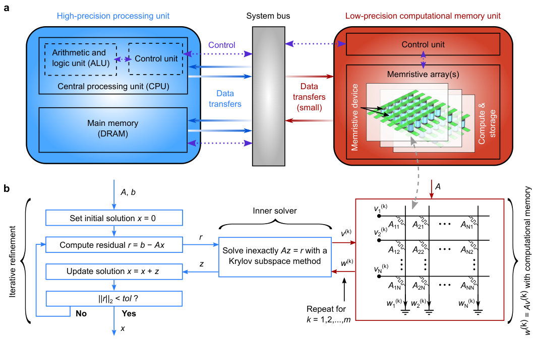 Figure 1
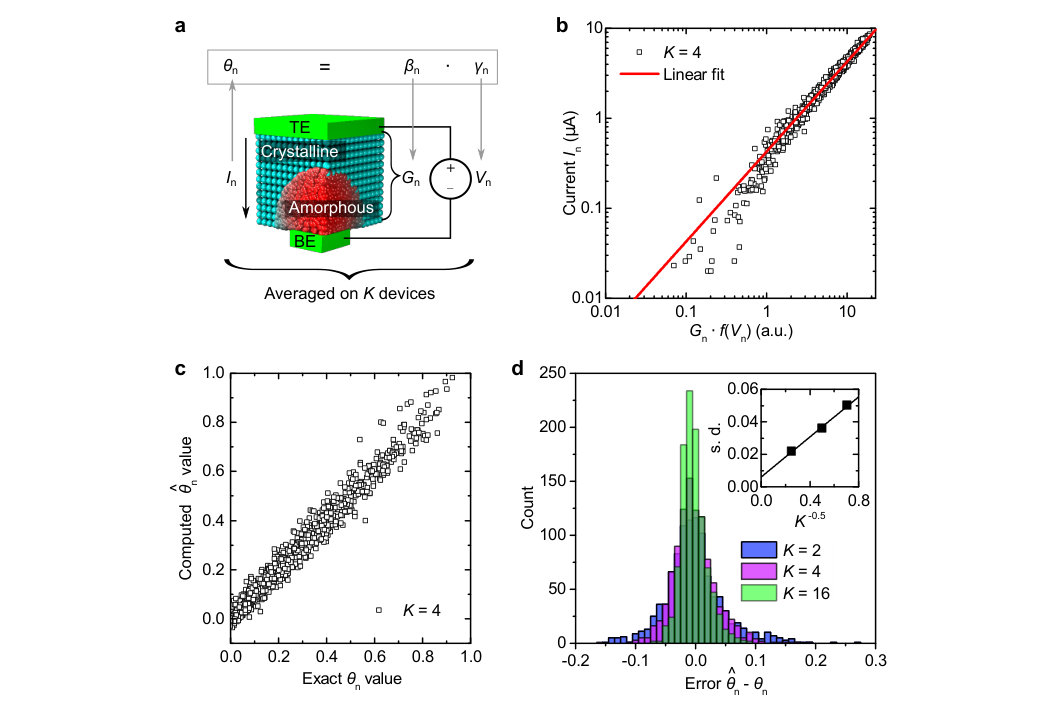 Figure 2
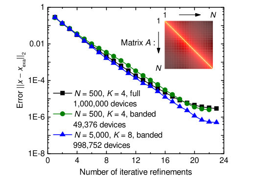 Figure 3
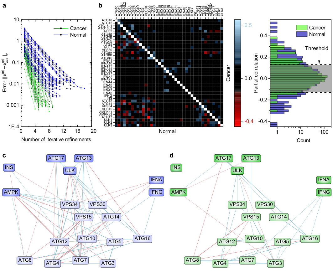 Figure 4
Peer Reviews
No public reviews on file for this paper yet. If you reviewed it on a platform where reviews are public (OpenReview, ICLR, NeurIPS, ICML), you can paste yours below so the community can read it here.
Videos
No videos yet. Explain this paper in a talk, walkthrough, or lecture? Add one.
Mixed-Precision In-Memory Computing
Manuel Le Gallo
IBM Research - Zurich, 8803 Rüschlikon, Switzerland
ETH Zurich, 8092 Zurich, Switzerland
Abu Sebastian
IBM Research - Zurich, 8803 Rüschlikon, Switzerland
Roland Mathis
IBM Research - Zurich, 8803 Rüschlikon, Switzerland
Matteo Manica
IBM Research - Zurich, 8803 Rüschlikon, Switzerland
ETH Zurich, 8092 Zurich, Switzerland
Heiner Giefers
IBM Research - Zurich, 8803 Rüschlikon, Switzerland
Tomas Tuma
IBM Research - Zurich, 8803 Rüschlikon, Switzerland
Costas Bekas
IBM Research - Zurich, 8803 Rüschlikon, Switzerland
Alessandro Curioni
IBM Research - Zurich, 8803 Rüschlikon, Switzerland
Evangelos Eleftheriou
IBM Research - Zurich, 8803 Rüschlikon, Switzerland
Abstract
As CMOS scaling reaches its technological limits, a radical departure from traditional von Neumann systems, which involve separate processing and memory units, is needed in order to significantly extend the performance of today’s computers. In-memory computing is a promising approach in which nanoscale resistive memory devices, organized in a computational memory unit, are used for both processing and memory. However, to reach the numerical accuracy typically required for data analytics and scientific computing, limitations arising from device variability and non-ideal device characteristics need to be addressed. Here we introduce the concept of mixed-precision in-memory computing, which combines a von Neumann machine with a computational memory unit. In this hybrid system, the computational memory unit performs the bulk of a computational task, while the von Neumann machine implements a backward method to iteratively improve the accuracy of the solution. The system therefore benefits from both the high precision of digital computing and the energy/areal efficiency of in-memory computing. We experimentally demonstrate the efficacy of the approach by accurately solving systems of linear equations, in particular, a system of equations using phase-change memory devices.
Nanoscale resistive memory devices, which are also referred to as memristive devices, can store information in their conductance states and can remember the history of the current that has flowed through them Strukov et al. (2008); Chua (2011); Wong and Salahuddin (2015). These devices form the basis of in-memory computing: an approach in which both information processing and storing computational data are performed on the same physical devices organized in a computational memory unit Di Ventra and Pershin (2013); Traversa and Di Ventra (2015); Sebastian et al. (2017); Le Gallo et al. (2017). With such systems, various physical mechanisms, including Ohm’s law and Kirchhoff’s circuit lawsHu et al. (2016); Li et al. (2018), chemically-driven phase transformationsXu et al. (2013), the pattern dynamics of ferroelectric domain switchingIevlev et al. (2014), and the physics of crystallizationCassinerio, Ciocchini, and Ielmini (2013); Sebastian, Le Gallo, and Krebs (2014) and meltingLoke et al. (2014) in phase-change materials, can be used to perform arithmeticWright et al. (2011); Xu et al. (2013); Hosseini et al. (2015); Hu et al. (2016) and logicalBorghetti et al. (2010); Kvatinsky et al. (2014); Cassinerio, Ciocchini, and Ielmini (2013); Loke et al. (2014) operations. Research on these devices has already led to the development of massively parallel, memory-centric hardware accelerators with applications ranging from image processing to healthcareBojnordi and Ipek (2016); Shafiee et al. (2016); Sheridan et al. (2017); Choi, Sheridan, and Lu (2015). However, building a computational memory unit that can solve practical problems in a reliable and accurate way remains challenging. Memristive devices suffer from significant inter-device variability and inhomogeneity across an arrayAmbrogio et al. (2014). Moreover, they exhibit intra-device variability and a randomness that is intrinsic to the way the devices operateFantini et al. (2013); Le Gallo et al. (2016). While this randomness can be exploited for certain types of computational tasksGaba et al. (2013); Tuma et al. (2016), the low precision associated with computational memory is prohibitive for many practical applications.
In this article, we introduce the concept of mixed-precision in-memory computing to address this issue. The concept is motivated by the observation that many computational tasks can be formulated as a sequence of two distinct parts. In the first part, an approximate solution is obtained. In the second part, the resulting error in the overall objective is calculated accurately. Then, based on this, the approximate solution is adapted (by repeating the first part). The first part typically has a high computational load, whereas the second part has a light computational load. By repeating this sequence several times, it is often possible to arrive at a solution with arbitrarily high accuracyBekas, Curioni, and Fedulova (2009). In a mixed-precision in-memory computing system, the idea is to use a low-precision computational memory unit to obtain the approximate solution of the first part and a high-precision processing unit to realize the second part (Fig. 1a). The expectation is that in this way we can benefit from an overall high areal and energy efficiency, because the bulk of the computation is still realized in a non-von Neumann manner, and still be able to achieve an arbitrarily high computational accuracy.
I Mixed-precision in-memory linear equation solver
To illustrate this concept, we present the problem of solving systems of linear equations. The problem is to find an unknown vector that satisfies the constraint
[TABLE]
Here is a non-singular matrix and is a known column vector of observations or measurements. The target of our study is the solution of dense covariance matrix problems, which are common in cognitive computing and data analytics.Bekas, Curioni, and Fedulova (2009) Such problems can be solved in the mixed-precision in-memory computing framework as shown in Fig. 1b. In a so-called iterative refinement algorithm, an initial solution is chosen as starting point and is iteratively updated with a low-precision error-correction term, . The error-correction term is computed by solving with an inexact inner solver using the residual , calculated with high precision.Klavík et al. (2014) The algorithm runs until the norm of the residual falls below a desired tolerance, .
For the inner solver, we use an iterative Krylov subspace method, such as the Conjugate Gradient method or the Generalized Minimum Residual (GMRES) method.Saad (2003) Krylov subspace methods are currently considered to be among the most important iterative techniques available for solving (1) with high dimensional matrices Saad (2003). These techniques rely on building a basis of the -th Krylov subspace . This basis is obtained by performing multiple matrix-vector multiplications with the matrix , and using to compute the next basis vector following an orthogonalization procedure. From this basis, the error-correction term, which is an approximation of , can be obtained.
In all Krylov subspace methods, the computationally most intensive operation is the matrix-vector multiplication . Hence, the key idea is to realize this operation in the computational memory unit, using a memristive crossbar array in which matrix is programmed as the conductance values of the memristive devices (Fig. 1b). This mode of computing is very efficient because the matrix-vector product is computed in situ in the memristive array, thereby eliminating any intermediate movement of data.Hu et al. (2016) Even if the computation realized this way is approximate and introduces perturbations in the inner solver, the outer iterative refinement algorithm ensures convergence to a high-accuracy solution.Klavík et al. (2014) The magnitude of the perturbations that can be tolerated is expected to decrease with increasing condition number of matrix (the condition number reflects how much the solution will change with respect to a change in ).Higham (2002)
II In-memory multiplications with PCM devices
For our experiments, we implemented the low-precision matrix-vector multiplication using a prototype chip containing one million phase-change memory (PCM) devices. PCM devices are resistive memory devices that can be programmed to achieve a desired conductance value by altering the amorphous/crystalline phase configuration within the device (Fig. 2a).Burr et al. (2016) The array consists of a matrix of 512 word lines 2048 bit lines integrated in 90-nm CMOS technology and connected in a crossbar configuration. Each crosspoint consists of a PCM device in series with an access transistor (see Methods and Supplementary Note I).
First, we investigated the scalar multiplication operation that forms the core of the matrix-vector multiplication performed with the PCM devices. Let , where and are numbers generated uniformly in . was mapped to an effective conductance value ( ratio at V) between approximately 0 and 50 S, and to a voltage between approximately 0.1 V and 0.3 V (see Supplementary Note II). Because the current is a slightly nonlinear function of the voltage in our PCM devices, the analogue multiplication was assumed to follow a “pseudo” Ohm’s law:
[TABLE]
In this equation, is an adjustable parameter and a polynomial function that approximates the current/voltage characteristics of the PCM devices (Supplementary Note II). The devices were programmed to the effective conductance using an iterative program-and-verify procedure (see Methods) and were subsequently read by applying a voltage . The experiment was repeated for different combinations of , and the results for each value of were averaged on devices (thus using devices in total). As shown in Fig. 2b, the computation of Eq. (2) is effectively realized over approximately 2 decades of current. The current, , can then be converted to an approximate value that represents the final result of the computation (Supplementary Note II), which is plotted in Fig. 2c against the exact result computed in double-precision floating point. The distributions of the error get narrower with increasing (see Fig. 2d), with the standard deviation scaling as (see inset) as dictated by the central limit theorem when averaging independent and identically distributed (iid) random variables. This indicates that the predominant part of the error comes from random perturbations in the current . Possible causes for such perturbations are inaccuracies in the iterative programming of the devices to the conductance , variability of the current/voltage characteristics across devices, inherent conductance variations and low-frequency noise arising from the amorphous phase-change material Koelmans et al. (2015).
The matrix-vector multiplication is a natural extension of the scalar multiplication in which the elements of matrix are coded into the conductance states of PCM devices. Because our experimental hardware only allows serial access to each individual crosspoint, only the element-by-element multiplications of the matrix-vector product were performed in hardware, whereas the sum was performed outside of the chip (Supplementary Note III). The accumulated effect of errors in this mode of computing is fundamentally different from that of rounding errors arising for example from fixed-point data conversions Higham (2002) (Supplementary Note IV). To prevent errors in the multiplication results due to the temporal evolution of the conductance values (drift)Sebastian et al. (2015); Gallo et al. (2016) of the PCM devices, we developed a calibration procedure which consists of periodically reading the summed conductance of a subset of the devices encoding matrix to account for a global conductance shift during an experiment (Supplementary Note V). This simple procedure is easily implemented in a crossbar array, and estimates the conductance variations directly from the devices without any assumptions on how the conductance changes.
III Accurately solving linear equations using PCM hardware
Next, we present the solution of (1) for model covariance matrices of different sizes defined as
[TABLE]
for and . Such matrices exhibit a decaying behavior that simulates decreasing correlation of features away from the main diagonal.Bekas, Curioni, and Fedulova (2009) We first programmed a full matrix (3) of size in our PCM chip with devices averaged per matrix element, using all one million PCM devices available, and executed the mixed-precision algorithm with Conjugate Gradient (CG) as inner solver for (see Methods). The experiment converged to the desired accuracy after 23 iterative refinements (see Fig. 3).
In the mixed-precision computing framework, one can work not only with an imprecise inner solver, but also with inexact input data.Klavík et al. (2014) For instance, because the elements far from the main diagonal of (3) are small, a reduced banded version of the matrix (with just entries on each side of the main diagonal) can be coded in the memristive array instead of the complete one. In this way, the inner solver works on an inexact version of matrix , which is coded in the memristive array, whereas the outer iterative refinement loop works towards finding the exact solution of (1) by using the full matrix for computing the residuals. Using this approach with matrix size and , we obtained a convergence rate almost identical to that without banding (see Fig. 3). We then tested this approach up to the maximum matrix size for which we could program the banded matrix in the PCM chip, and obtained the desired convergence for using (see Fig. 3). 23 high-precision matrix-vector multiplications were required to solve this problem with mixed-precision in-memory computing, whereas 50 matrix-vector multiplications are needed when performing a single run of the CG algorithm in high precision to obtain the same solution accuracy. Therefore, the mixed-precision in-memory computing solution indeed reduces the number of floating point operations and associated data transfers needed to solve the problem compared to a conventional von Neumann implementation in high precision.
Because of the high-precision iterative refinement, the maximum achievable accuracy of the mixed-precision in-memory computing system is limited only by the precision of the high-precision processing unit, but not by the precision of the computational memory unit. The minimum error reached experimentally for when setting is , which is limited by the machine precision of the high-precision processing unit we use (Supplementary Note VI). Several methods can be used to speed up the convergence of the mixed-precision algorithm further and allowed us to obtain convergence for even larger matrix sizes of up to (Supplementary Note VI).
In addition, we tested the mixed-precision algorithm on a practical problem for which matrix was built from real-world data. For this, we used RNA expression measurements of genes obtained from cancer patients, publicly available from The Cancer Genome Atlas (TCGA) project (see Methods). We focused our investigation on 40 genes reported in the manually curated autophagy pathway of the Kyoto Encyclopedia of Genes and Genomes (KEGG). Autophagy plays opposing roles in cancer by both acting as a tumor suppressor by degrading damaged proteins and organelles as well as enabling tumors to tolerate metabolic stress Mathew, Karantza-Wadsworth, and White (2007); Yang et al. (2011). To infer and compare the networks of gene interactions (interactomes) from normal and cancer tissues, we calculated the partial correlations between the genes by computing the inverse covariance matrix from 946 normal tissue samples and from 946 cancer tissue samples (see Methods). Given the covariance matrix of the 40 genes, can be obtained by solving for , where has all entries equal to zero except the -th one, which is 1, and is the resulting -th column of .
We programmed the covariance matrix in the PCM chip and used mixed-precision in-memory computing with GMRES as inner solver to solve the 40 linear equations (see Methods). The procedure was repeated for both cancer and normal tissues. The algorithm converged to the desired precision for all 40 linear systems solved (see Fig. 4a) and the resulting matrix was sufficiently accurate for computing the interactome (the interactomes obtained with the exact and computed are identical). The computed partial correlations of the 40 genes studied and their distributions are shown in Fig. 4b. While some of the gene interactions are preserved between the cancer and normal tissues, the cancer network exhibits a different connectivity pattern (see Fig. 4c and 4d). In the normal tissue, the upstream signals INS, AMPK, ULK, ATG13, ATG17, IFNA and IFNG (dark colored) correlate with many of the downstream targets (light colored) known to be involved in the formation of autophagosomes, the molecular agents of autophagy. The partial correlations computed on cancerous tissue yield a sparsely connected network, implying an altered regulation pattern, as is commonly observed in cancer West et al. (2012); Schramm, Kannabiran, and König (2010); Hong et al. (2013).
IV Performance assessment and current limitations
The above demonstration highlights the importance of linear analysis in problems associated with cognitive computing and data analytics. The fact that such computation can be performed partly with computational memory without sacrificing the overall computational accuracy opens up exciting new avenues towards energy-efficient large-scale data analytics, in which the massive data transfers inherent to the traditional von Neumann architecture have become the most energy-hungry part. Such solutions are much needed because analyzing the ever-growing datasets we produce will quickly increase the computational load to the exascale level if standard techniques are to be used.Bekas, Curioni, and Fedulova (2009)
The problems tackled in this work were well-conditioned and of relatively small scale because of the limited size and precision of our hardware. Scale-up strategies include building larger arrays and/or operating several of them in parallel. To address problems with a broader range of condition numbers, it will be necessary to increase the precision of the computational memory unit beyond that achieved in the present work to allow the Krylov-subspace inner solver to converge more easily Klavík et al. (2014). Possible avenues are improving the memristive device characteristics with respect to variability and conductance noise Koelmans et al. (2015), mapping a single column of the matrix to multiple physical columns of an array encoding different bits (Supplementary Note III), and using error-correction techniques within the computational memory unit Feinberg, Wang, and Ipek (2018). The efficiency and robustness of iterative Krylov-subspace solvers can also be improved by using preconditioning techniques Saad (2003). Moreover, although we restricted our experiments to diagonally-dominant covariance type matrices, it is not a limitation of the mixed-precision in-memory computing concept, which can be used to solve (1) for more general types of matrices provided that the convergence conditionsSaad (2003) of the chosen Krylov subspace solver are met. In fact, while the CG method requires that the matrix is symmetric and positive-definite, the GMRES method that we used on the RNA data can deal with a much broader family of problems, in particular non-symmetric matrices, but at a slightly higher computational complexity than CG Saad (2003).
Finally, we performed a detailed study to compare the energy efficiency of the mixed-precision in-memory computing system with that of conventional von Neumann implementations (Supplementary Note VII.A). We implemented all data conversions and data transfers between the high-precision and computational memory units as well as all additional floating-point operations needed to solve (1) with the algorithm of Fig. 1b. We then experimentally measured the runtime and power consumption of the system using both a IBM POWER8 CPU and a NVIDIA P100 GPU as high-precision processing unit. In those measurements, it was assumed that the operations in the computational memory unit consume negligible time and energy compared to the operations performed in the high-precision computing unit, thus providing an upper bound on the achievable performance of the system. Our analysis shows that mixed-precision in-memory computing can outperform both CPU-based and GPU-based implementations that use only high-precision arithmetic in terms of both time and energy to solution. For matrix (3), the maximum measured dynamic energy gains range from with the precision of the computational memory unit comparable to that of our current PCM chip, up to when assuming two orders of magnitude less noiseKoelmans et al. (2015) in the computational memory unit. Note that those numbers are strongly tied to matrix and the right-hand side used, and that in general higher energy gains are expected the more ill-conditioned the matrix is Anzt, Heuveline, and Rocker (2012). The achievable performance depends on the ratio between the number of iterations required in the high-precision-only implementation versus the number of iterative refinements performed in the mixed-precision in-memory computing algorithm, which in turn depends on both the precision of the computational memory unit and the actual problem that is solved (Supplementary Note VII.A).
Subsequently, we derived specifications which should be met by the computational memory unit in order to achieve a system performance close to the aforementioned upper bound in terms of speed. Assuming a crossbar size of cells, we expect that operating 10 crossbars in parallel at a cycle time of 1 s or less should allow the mixed-precision in-memory computing system to reach optimal performance in terms of speed (Supplementary Note VII.B). We believe that those specifications should be within the reach of existing technology because circuit simulations show that memristive crossbars can be run at a frequency of 10 MHz Hu et al. (2016) and memristive crossbars with ns latency have already been demonstrated Li et al. (2018). During the execution of the mixed-precision algorithm, only read operations are performed on the memristive array, which consume much less energy than programming ( fJ per PCM device), and hence the additional power overhead from the crossbar is expected to be minimal compared to that of the high-precision processing unit (Supplementary Note VII.B). Nonetheless, efficient designs of the crossbar peripheral circuitry and I/O converters will be of utmost importance to ensure that the computational memory unit meets those specifications.
Moreover, to assess the capability of computational memory to compete with already existing low-precision CMOS-based accelerators for performing matrix-vector multiplications, we designed a low-precision 4-bit matrix-vector multiplier on a field-programmable gate array (FPGA) with an accuracy comparable to what could be obtained with our current prototype PCM chip. Our analysis shows that even when all matrix coefficients are stored in the FPGA memory (thus neglecting any off-chip data transfers), a memristive crossbar array based on devices similar to our prototype PCM chip for performing analogue matrix-vector multiplications could already offer up to 80 times lower energy consumption than the FPGA solution (Supplementary Note VIII).
V Conclusions
In summary, we have introduced the concept of mixed-precision in-memory computing to address the inherent imprecision associated with computational memory. The hybrid system comprises a computational memory unit, which performs the bulk of a given computational task, and a high-precision processing unit which implements a backward method to iteratively improve the accuracy of the solution. In this way, it is possible to achieve an arbitrarily high solution accuracy with the bulk of the computation realized as low-precision in-memory computing. We have experimentally demonstrated this concept by solving systems of linear equations using a PCM chip to perform analogue matrix-vector multiplications, on both model covariance matrices and a practical problem in which the matrix was built from real-world RNA expression data. The next steps will be to generalize mixed-precision in-memory computing beyond the application domain of solving systems of linear equations to other computationally intensive tasks arising in automatic control, optimization problems, machine learning, deep learningNandakumar et al. (2017), and signal processing.
Methods
Experimental platform.
The experimental platform is built around a prototype PCM chip that comprises 3 million PCM devices. The PCM array is organized as a matrix of word lines (WL) and bit lines (BL). In addition to the PCM devices, the prototype chip integrates the circuitry for device addressing and for write and read operations. The PCM chip is interfaced to a hardware platform comprising two field programmable gate array (FPGA) boards and an analog-front-end (AFE) board. The AFE board provides the power supplies as well as the voltage and current reference sources for the PCM chip. The FPGA boards are used to implement overall system control and data management as well as the interface with the data processing unit. The experimental platform is operated from a host computer, and a Matlab environment is used to coordinate the experiments. The algorithms used to solve the linear equations and all data conversions are implemented in Matlab software.
The PCM devices were integrated into the chip in 90-nm CMOS technology using the key-hole process described in Ref. Breitwisch et al., 2007. The phase-change material is doped Ge2Sb2Te5. The bottom electrode has a radius of nm and a length of nm. The phase-change material is nm thick and extends to the top electrode, whose radius is nm. Two types of devices are available on-chip that differ in the size of the access transistor. The first sub-array contains 2 million devices, and each device is accessed by a 240 nm-wide transistor. The second sub-array contains 1 million devices, and two 240 nm-wide access transistors are used in parallel per PCM element. All experiments performed in this work were done on the second sub-array, which is organized as a matrix of 512 WL and 2048 BL.
A PCM device is selected by serially addressing a WL and a BL. To read a PCM device, the selected BL is biased to a constant voltage (typically mV) by a voltage regulator via a voltage generated off chip. The sensed current is integrated by a capacitor, and the resulting voltage is then digitized by the on-chip 8-bit cyclic analog-to-digital converter (ADC). The total duration of one read is s. The readout characteristic is calibrated via on-chip reference polysilicon resistors. To program a PCM device, a voltage generated off chip is converted on chip into a programming current. This current is then mirrored into the selected BL for the desired duration of the programming pulse. Each programming pulse is a box-type rectangular pulse with duration of 400 ns and an amplitude varying between 0 and 500 A. Iterative programming involving a sequence of program-and-verify steps is used to program the PCM devices to the desired conductance values.Papandreou et al. (2011) After each programming pulse, a verify step is performed, and the value of the device conductance programmed in the preceding iteration is read at a voltage of 0.2 V. The programming current applied to the PCM device in the subsequent iteration is adapted according to the sign of the value of the error between the target level and the read value of the device conductance. The programming sequence ends when the error between the target conductance and the programmed conductance of the device is smaller than a margin of 1.74 S or when the maximum number of iterations (20) has been reached. The total duration of one program-and-verify step is approx. s.
More details about the hardware platform and chip characterization results can be found in Supplementary Note I.
Solving the linear system for model covariance matrices.
We solved the linear system with mixed-precision in-memory computing for the covariance matrices defined by Eq. (3). The entries of were generated uniformly in . We used the following Conjugate Gradient (CG) method as the inner Krylov-subspace solver:
The final solution is given by . denotes the matrix which is coded in the PCM chip. When the full matrix is coded in the PCM chip, . When a reduced banded version of is coded in the PCM chip, we have
[TABLE]
All nonzero elements of were coded in the PCM chip using devices averaged per element according to the procedure described in Supplementary Note III. The matrix-vector multiplication was performed with the chip as described in Supplementary Note III. The number of CG iterations was set to for and to for . The tolerance of the iterative refinement algorithm was set to . The drift calibration procedure described in Supplementary Note V was performed at every first iteration of Algorithm 1 on devices to prevent errors in the multiplication results due to conductance drift of the phase-change devices.
Estimation of gene interactions from RNA measurements.
We used RNA-Seq (Illumina HiSeq 2000 RNA Sequencing Version 2) Level 3 data from TCGA (http://cancergenome.nih.gov/) project, normalized with RSEMLi and Dewey (2011). The 40 genes studied were selected from the autophagy pathway (hsa04140) curated by KEGG (http://www.genome.jp/). We considered tissue samples across different cancer types. The number of normal samples (946) was smaller than the number of cancer samples (11935). To compare networks estimated with the same sample size, we subsampled 946 RNA-Seq cancer profiles to match the size of the normal samples. To ensure that no bias was introduced by subsampling, we performed a Kolmogorov–Smirnov test on the subsampled distributions, which showed no evidence of difference (, with Bonferroni correction). The sample covariance between gene and gene was computed as
[TABLE]
where indicates the expression value of gene in sample and is the mean expression of gene across all samples.
The inverse covariance matrix was computed from covariance matrix by solving for with mixed-precision in-memory computing. All entries are equal to zero except the -th one, which is 1, and is the resulting -th column of . We apply a diagonal preconditioner on the linear system, thus solving the problem . Then, we define matrix as
[TABLE]
Note that all diagonal elements of are set to 0. All nonzero elements of were coded in the PCM chip using 4 devices averaged per element according to the procedure described in Supplementary Note III. We used the following Generalized Minimum Residual (GMRES) method as the inner Krylov-subspace solver:
The final solution is given by . The matrix-vector multiplication was performed with the chip as described in Supplementary Note III. Line 4 of Algorithm 2 adds the remaining term to , where is the identity matrix (concretely, we approximate by ). This avoids coding the diagonal elements of , which are all 1s, in the memristive array to prevent unnecessary large perturbations in which would come from inexact computing of . The number of GMRES iterations was set to . The tolerance of the iterative refinement algorithm was set to . The drift calibration procedure described in Supplementary Note V was performed at every first iteration of Algorithm 2 to prevent errors in the multiplication results due to conductance drift of the phase-change devices.
The partial correlation between gene and gene was computed from the inverse covariance as
[TABLE]
For the interactome visualization, we considered interactions only for which the magnitude of the partial correlations was larger than a threshold , corresponding to 90th percentile of the normals. In the graphs, genes were grouped following the KEGG Orthology () System. We defined a set of interactions between groups:
[TABLE]
where and contain gene indexes as they appear in the partial correlations matrix and correspond to the groups defined in KEGG (e.g. AMPK or ULK). The strength of the correlation between groups was then defined by averaging the partial correlations:
[TABLE]
Finally, the graphs were built using the partial correlations values and the strength of the correlations between groups as defined above. This allowed us to connect interacting genes and groups with a variable intensity in a more compact representation.
Data availability.
The data that support the plots within this paper and other findings of this study are available from the corresponding author upon reasonable request.
References
- Strukov et al. (2008) D. B. Strukov, G. S. Snider, D. R. Stewart, and R. S. Williams, “The missing memristor found,” Nature 453, 80–83 (2008).
- Chua (2011) L. Chua, “Resistance switching memories are memristors,” Applied Physics A 102, 765–783 (2011).
- Wong and Salahuddin (2015) H.-S. P. Wong and S. Salahuddin, “Memory leads the way to better computing,” Nature Nanotechnology 10, 191–194 (2015).
- Di Ventra and Pershin (2013) M. Di Ventra and Y. V. Pershin, “The parallel approach,” Nature Physics 9, 200–202 (2013).
- Traversa and Di Ventra (2015) F. L. Traversa and M. Di Ventra, “Universal memcomputing machines,” IEEE Transactions on Neural Networks and Learning Systems 26, 2702–2715 (2015).
- Sebastian et al. (2017) A. Sebastian, T. Tuma, N. Papandreou, M. Le Gallo, L. Kull, T. Parnell, and E. Eleftheriou, “Temporal correlation detection using computational phase-change memory,” Nature Communications 8, 1115 (2017).
- Le Gallo et al. (2017) M. Le Gallo, A. Sebastian, G. Cherubini, H. Giefers, and E. Eleftheriou, “Compressed sensing recovery using computational memory,” in Proceedings of the IEEE International Electron Devices Meeting (IEDM) (2017) pp. 28.3.1–28.3.4.
- Hu et al. (2016) M. Hu, J. P. Strachan, Z. Li, E. M. Grafals, N. Davila, C. Graves, S. Lam, N. Ge, J. J. Yang, and R. S. Williams, “Dot-product engine for neuromorphic computing: Programming 1T1M crossbar to accelerate matrix-vector multiplication,” in Proceedings of the 53rd Annual Design Automation Conference (DAC) (2016) pp. 19:1–19:6.
- Li et al. (2018) C. Li, M. Hu, Y. Li, H. Jiang, N. Ge, E. Montgomery, J. Zhang, W. Song, N. Dávila, C. E. Graves, et al., “Analogue signal and image processing with large memristor crossbars,” Nature Electronics 1, 52 (2018).
- Xu et al. (2013) H. Xu, Y. Xia, K. Yin, J. Lu, Q. Yin, J. Yin, L. Sun, and Z. Liu, “The chemically driven phase transformation in a memristive abacus capable of calculating decimal fractions,” Scientific Reports 3, 1230 (2013).
- Ievlev et al. (2014) A. Ievlev, S. Jesse, A. Morozovska, E. Strelcov, E. Eliseev, Y. Pershin, A. Kumar, V. Y. Shur, and S. Kalinin, “Intermittency, quasiperiodicity and chaos in probe-induced ferroelectric domain switching,” Nature Physics 10, 59–66 (2014).
- Cassinerio, Ciocchini, and Ielmini (2013) M. Cassinerio, N. Ciocchini, and D. Ielmini, “Logic computation in phase change materials by threshold and memory switching,” Advanced Materials 25, 5975–5980 (2013).
- Sebastian, Le Gallo, and Krebs (2014) A. Sebastian, M. Le Gallo, and D. Krebs, “Crystal growth within a phase change memory cell,” Nature Communications 5, 4314 (2014).
- Loke et al. (2014) D. Loke, J. M. Skelton, W.-J. Wang, T.-H. Lee, R. Zhao, T.-C. Chong, and S. R. Elliott, “Ultrafast phase-change logic device driven by melting processes,” Proceedings of the National Academy of Sciences 111, 13272–13277 (2014).
- Wright et al. (2011) C. D. Wright, Y. Liu, K. I. Kohary, M. M. Aziz, and R. J. Hicken, “Arithmetic and biologically-inspired computing using phase-change materials,” Advanced Materials 23, 3408–3413 (2011).
- Hosseini et al. (2015) P. Hosseini, A. Sebastian, N. Papandreou, C. D. Wright, and H. Bhaskaran, “Accumulation-based computing using phase-change memories with FET access devices,” IEEE Electron Device Letters 36, 975–977 (2015).
- Borghetti et al. (2010) J. Borghetti, G. S. Snider, P. J. Kuekes, J. J. Yang, D. R. Stewart, and R. S. Williams, “‘Memristive’ switches enable ‘stateful’ logic operations via material implication,” Nature 464, 873–876 (2010).
- Kvatinsky et al. (2014) S. Kvatinsky, D. Belousov, S. Liman, G. Satat, N. Wald, E. G. Friedman, A. Kolodny, and U. C. Weiser, “MAGIC: Memristor-aided logic,” IEEE Transactions on Circuits and Systems II: Express Briefs 61, 895–899 (2014).
- Bojnordi and Ipek (2016) M. N. Bojnordi and E. Ipek, “Memristive Boltzmann machine: A hardware accelerator for combinatorial optimization and deep learning,” in Proceedings of the IEEE International Symposium on High Performance Computer Architecture (HPCA) (2016) pp. 1–13.
- Shafiee et al. (2016) A. Shafiee, A. Nag, N. Muralimanohar, R. Balasubramonian, J. P. Strachan, M. Hu, R. S. Williams, and V. Srikumar, “ISAAC: A convolutional neural network accelerator with in-situ analog arithmetic in crossbars,” in Proceedings of the 43rd International Symposium on Computer Architecture (2016) pp. 14–26.
- Sheridan et al. (2017) P. M. Sheridan, F. Cai, C. Du, W. Ma, Z. Zhang, and W. D. Lu, “Sparse coding with memristor networks.” Nature Nanotechnology 12, 784–789 (2017).
- Choi, Sheridan, and Lu (2015) S. Choi, P. Sheridan, and W. D. Lu, “Data clustering using memristor networks,” Scientific Reports 5, 10492 (2015).
- Ambrogio et al. (2014) S. Ambrogio, S. Balatti, A. Cubeta, A. Calderoni, N. Ramaswamy, and D. Ielmini, “Statistical fluctuations in HfOx resistive-switching memory: Part I-set/reset variability,” IEEE Transactions on Electron Devices 61, 2912–2919 (2014).
- Fantini et al. (2013) A. Fantini, L. Goux, R. Degraeve, D. Wouters, N. Raghavan, G. Kar, A. Belmonte, Y.-Y. Chen, B. Govoreanu, and M. Jurczak, “Intrinsic switching variability in HfO2 RRAM,” in 2013 5th IEEE International Memory Workshop (IEEE, 2013) pp. 30–33.
- Le Gallo et al. (2016) M. Le Gallo, T. Tuma, F. Zipoli, A. Sebastian, and E. Eleftheriou, “Inherent stochasticity in phase-change memory devices,” in Proc. of the European Solid-State Device Research Conference (ESSDERC) (IEEE, 2016) pp. 373–376.
- Gaba et al. (2013) S. Gaba, P. Sheridan, J. Zhou, S. Choi, and W. Lu, “Stochastic memristive devices for computing and neuromorphic applications,” Nanoscale 5, 5872–5878 (2013).
- Tuma et al. (2016) T. Tuma, A. Pantazi, M. Le Gallo, A. Sebastian, and E. Eleftheriou, “Stochastic phase-change neurons,” Nature Nanotechnology 11, 693 –699 (2016).
- Bekas, Curioni, and Fedulova (2009) C. Bekas, A. Curioni, and I. Fedulova, “Low cost high performance uncertainty quantification,” in Proceedings of the 2nd Workshop on High Performance Computational Finance (ACM, 2009) pp. 8:1–8:8.
- Klavík et al. (2014) P. Klavík, A. C. I. Malossi, C. Bekas, and A. Curioni, “Changing computing paradigms towards power efficiency,” Philosophical Transactions of the Royal Society of London A: Mathematical, Physical and Engineering Sciences 372, 20130278 (2014).
- Saad (2003) Y. Saad, Iterative methods for sparse linear systems (Siam, 2003).
- Higham (2002) N. J. Higham, Accuracy and stability of numerical algorithms (Siam, 2002).
- Burr et al. (2016) G. W. Burr, M. J. Brightsky, A. Sebastian, H.-Y. Cheng, J.-Y. Wu, S. Kim, N. E. Sosa, N. Papandreou, H.-L. Lung, H. Pozidis, et al., “Recent progress in phase-change memory technology,” IEEE Journal on Emerging and Selected Topics in Circuits and Systems 6, 146–162 (2016).
- Koelmans et al. (2015) W. W. Koelmans, A. Sebastian, V. P. Jonnalagadda, D. Krebs, L. Dellmann, and E. Eleftheriou, “Projected phase-change memory devices,” Nature communications 6, 8181 (2015).
- Sebastian et al. (2015) A. Sebastian, D. Krebs, M. Le Gallo, H. Pozidis, and E. Eleftheriou, “A collective relaxation model for resistance drift in phase change memory cells,” in International Reliability Physics Symposium (IRPS) (2015) pp. MY.5.1–MY.5.6.
- Gallo et al. (2016) M. L. Gallo, A. Sebastian, D. Krebs, M. Stanisavljevic, and E. Eleftheriou, “The complete time/temperature dependence of I-V drift in PCM devices,” in International Reliability Physics Symposium (IRPS) (2016) pp. MY–1–1–MY–1–6.
- Mathew, Karantza-Wadsworth, and White (2007) R. Mathew, V. Karantza-Wadsworth, and E. White, “Role of autophagy in cancer,” Nature Reviews Cancer 7, 961–967 (2007).
- Yang et al. (2011) Z. J. Yang, C. E. Chee, S. Huang, and F. A. Sinicrope, “The role of autophagy in cancer: therapeutic implications,” Molecular Cancer Therapeutics 10, 1533–1541 (2011).
- West et al. (2012) J. West, G. Bianconi, S. Severini, and A. E. Teschendorff, “Differential network entropy reveals cancer system hallmarks,” Scientific Reports 2, 802 (2012).
- Schramm, Kannabiran, and König (2010) G. Schramm, N. Kannabiran, and R. König, “Regulation patterns in signaling networks of cancer,” BMC Systems Biology 4, 1 (2010).
- Hong et al. (2013) S. Hong, X. Chen, L. Jin, and M. Xiong, “Canonical correlation analysis for RNA-seq co-expression networks,” Nucleic Acids Research 41, e95–e95 (2013).
- Feinberg, Wang, and Ipek (2018) B. Feinberg, S. Wang, and E. Ipek, “Making memristive neural network accelerators reliable,” in Proceedings of the IEEE International Symposium on High Performance Computer Architecture (HPCA) (2018).
- Anzt, Heuveline, and Rocker (2012) H. Anzt, V. Heuveline, and B. Rocker, “Mixed precision iterative refinement methods for linear systems: Convergence analysis based on krylov subspace methods,” in Applied Parallel and Scientific Computing (Springer, 2012) pp. 237–247.
- Nandakumar et al. (2017) S. R. Nandakumar, M. Le Gallo, I. Boybat, B. Rajendran, A. Sebastian, and E. Eleftheriou, “Mixed-precision training of deep neural networks using computational memory,” arXiv preprint arXiv:1712.01192 (2017).
- Breitwisch et al. (2007) M. Breitwisch, T. Nirschl, C. Chen, Y. Zhu, M. Lee, M. Lamorey, G. Burr, E. Joseph, A. Schrott, J. Philipp, et al., “Novel lithography-independent pore phase change memory,” in Proc. IEEE Symposium on VLSI Technology (2007) pp. 100–101.
- Papandreou et al. (2011) N. Papandreou, H. Pozidis, A. Pantazi, A. Sebastian, M. Breitwisch, C. Lam, and E. Eleftheriou, “Programming algorithms for multilevel phase-change memory,” in Proceedings of the International Symposium on Circuits and Systems (ISCAS) (2011) pp. 329–332.
- Li and Dewey (2011) B. Li and C. N. Dewey, “RSEM: accurate transcript quantification from RNA-Seq data with or without a reference genome,” BMC Bioinformatics 12, 1 (2011).
Acknowledgments
We thank C. Malossi, M. Rodriguez, C. Hagleitner, L. Kull and T. Toifl for discussions; N. Papandreou, A. Athmanathan and U. Egger for experimental help; T. Delbruck for reviewing the manuscript; and C. Bolliger for help with the preparation of the manuscript. A. S. would like to acknowledge funding from the European Research Council (ERC) under the European Union’s Horizon 2020 research and innovation programme (grant agreement No. 682675).
Author contributions
M.L., A.S., T.T., C.B., A.C. and E.E. conceived the concept of mixed-precision in-memory computing. M.L., A.S. and C.B. designed the research. M.L. implemented the mixed-precision in-memory computing system and performed all experiments. M.L., R.M. and M.M. performed the research on the RNA expression data. H.G. performed the evaluation of the runtime and energy consumption. All authors contributed to the analysis and interpretation of the results. M.L. and A.S. co-wrote the manuscript based on the input from all authors.
Competing interests
The authors declare no competing financial interests.
The reference list from the paper itself. Each links out to its DOI / PubMed record.
- 1Strukov et al. (2008) D. B. Strukov, G. S. Snider, D. R. Stewart, and R. S. Williams, “The missing memristor found,” Nature 453 , 80–83 (2008).
- 2Chua (2011) L. Chua, “Resistance switching memories are memristors,” Applied Physics A 102 , 765–783 (2011).
- 3Wong and Salahuddin (2015) H.-S. P. Wong and S. Salahuddin, “Memory leads the way to better computing,” Nature Nanotechnology 10 , 191–194 (2015).
- 4Di Ventra and Pershin (2013) M. Di Ventra and Y. V. Pershin, “The parallel approach,” Nature Physics 9 , 200–202 (2013).
- 5Traversa and Di Ventra (2015) F. L. Traversa and M. Di Ventra, “Universal memcomputing machines,” IEEE Transactions on Neural Networks and Learning Systems 26 , 2702–2715 (2015).
- 6Sebastian et al. (2017) A. Sebastian, T. Tuma, N. Papandreou, M. Le Gallo, L. Kull, T. Parnell, and E. Eleftheriou, “Temporal correlation detection using computational phase-change memory,” Nature Communications 8 , 1115 (2017).
- 7Le Gallo et al. (2017) M. Le Gallo, A. Sebastian, G. Cherubini, H. Giefers, and E. Eleftheriou, “Compressed sensing recovery using computational memory,” in Proceedings of the IEEE International Electron Devices Meeting (IEDM) (2017) pp. 28.3.1–28.3.4.
- 8Hu et al. (2016) M. Hu, J. P. Strachan, Z. Li, E. M. Grafals, N. Davila, C. Graves, S. Lam, N. Ge, J. J. Yang, and R. S. Williams, “Dot-product engine for neuromorphic computing: Programming 1T 1M crossbar to accelerate matrix-vector multiplication,” in Proceedings of the 53rd Annual Design Automation Conference (DAC) (2016) pp. 19:1–19:6.