Composite fermion basis for two-component Bose gases
Ola Liab{\o}tr{\o}, Marius Ladeg{\aa}rd Meyer

TL;DR
This paper develops a mathematically rigorous basis for composite fermion states in two-component Bose gases, enabling better analysis of their structure and overlaps with exact solutions in quantum Hall systems.
Contribution
It introduces multiple methods to construct a linearly independent basis for simple CF states, addressing a key mathematical challenge in the field.
Findings
Constructed linearly independent basis for CF states
Analyzed the structure of lowest-lying states
Studied overlap scaling with exact wave functions
Abstract
Despite its success, the composite fermion (CF) construction possesses some mathematical features that have, until recently, not been fully understood. In particular, it is known to produce wave functions that are not necessarily orthogonal, or even linearly independent, after projection to the lowest Landau level. While this is usually not a problem in practice in the quantum Hall regime, we have previously shown that it presents a technical challenge for rotating Bose gases with low angular momentum. These are systems where the CF approach yields surprisingly good approximations to the exact eigenstates of weak short-range interactions, and so solving the problem of linearly dependent wave functions is of interest. It can also be useful for studying higher bands of fermionic quantum Hall states. Here we present several ways of constructing a basis for the space of so-called "simple"…
Click any figure to enlarge with its caption.
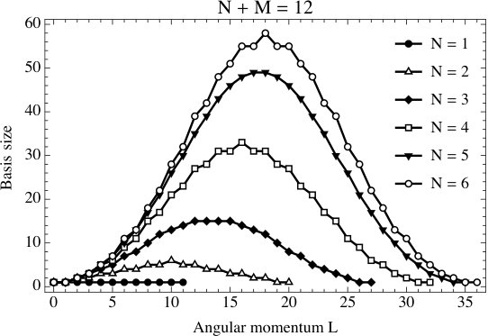 Figure 1
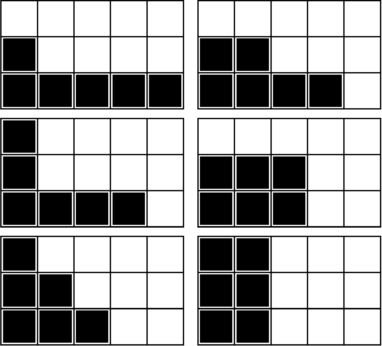 Figure 2
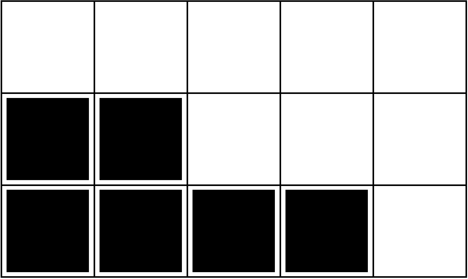 Figure 3
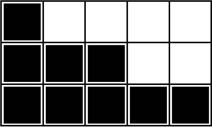 Figure 4
 Figure 5
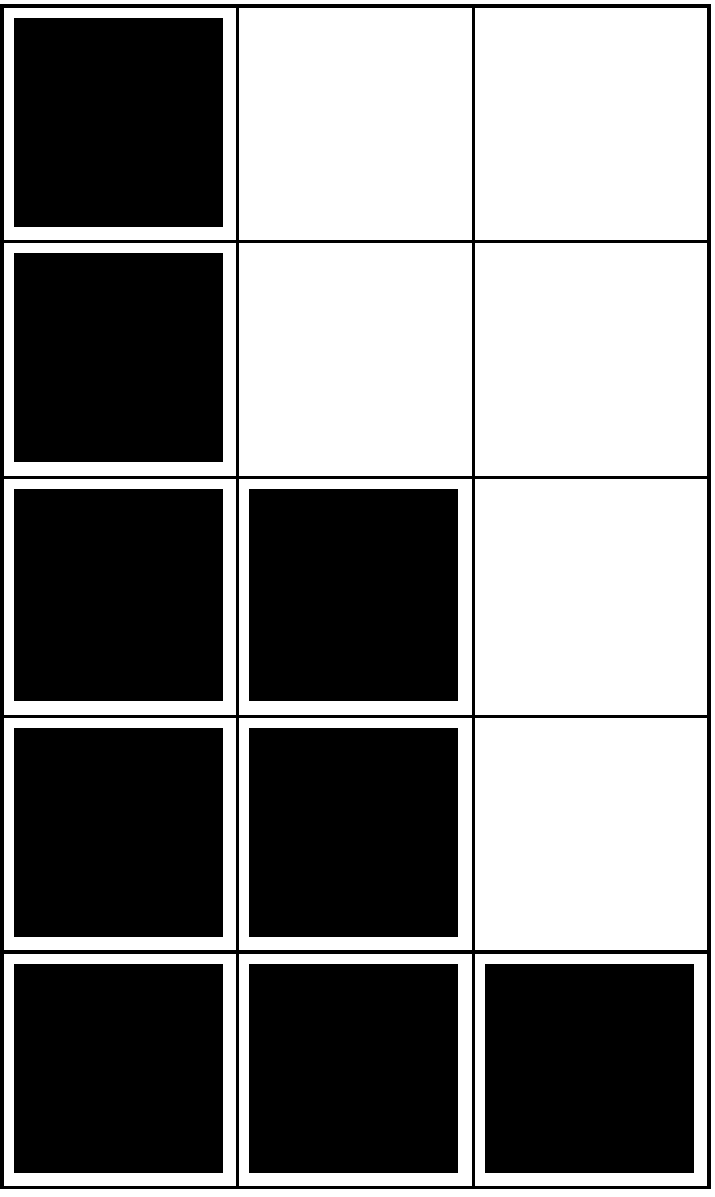 Figure 6
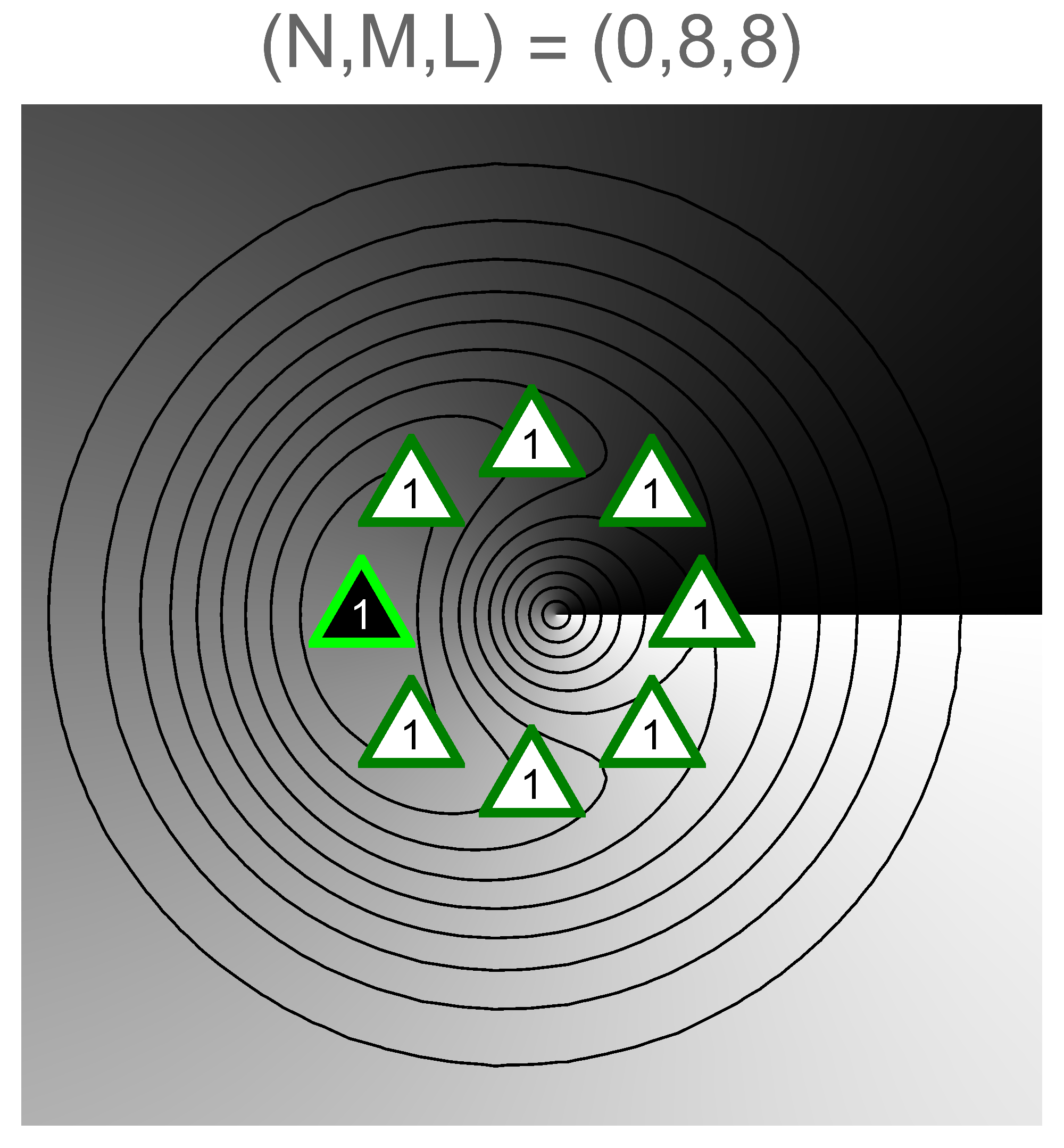 Figure 7
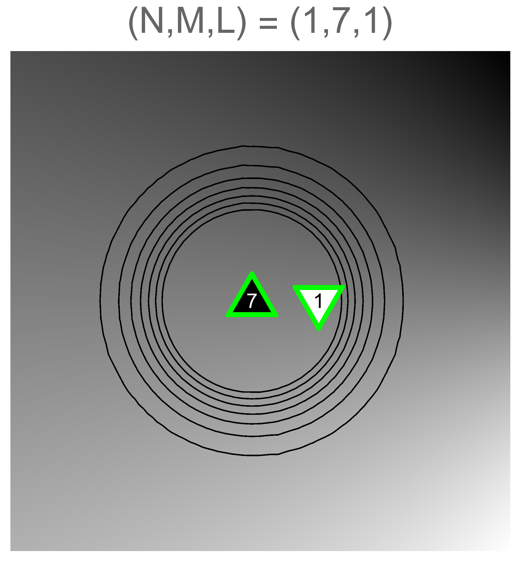 Figure 8
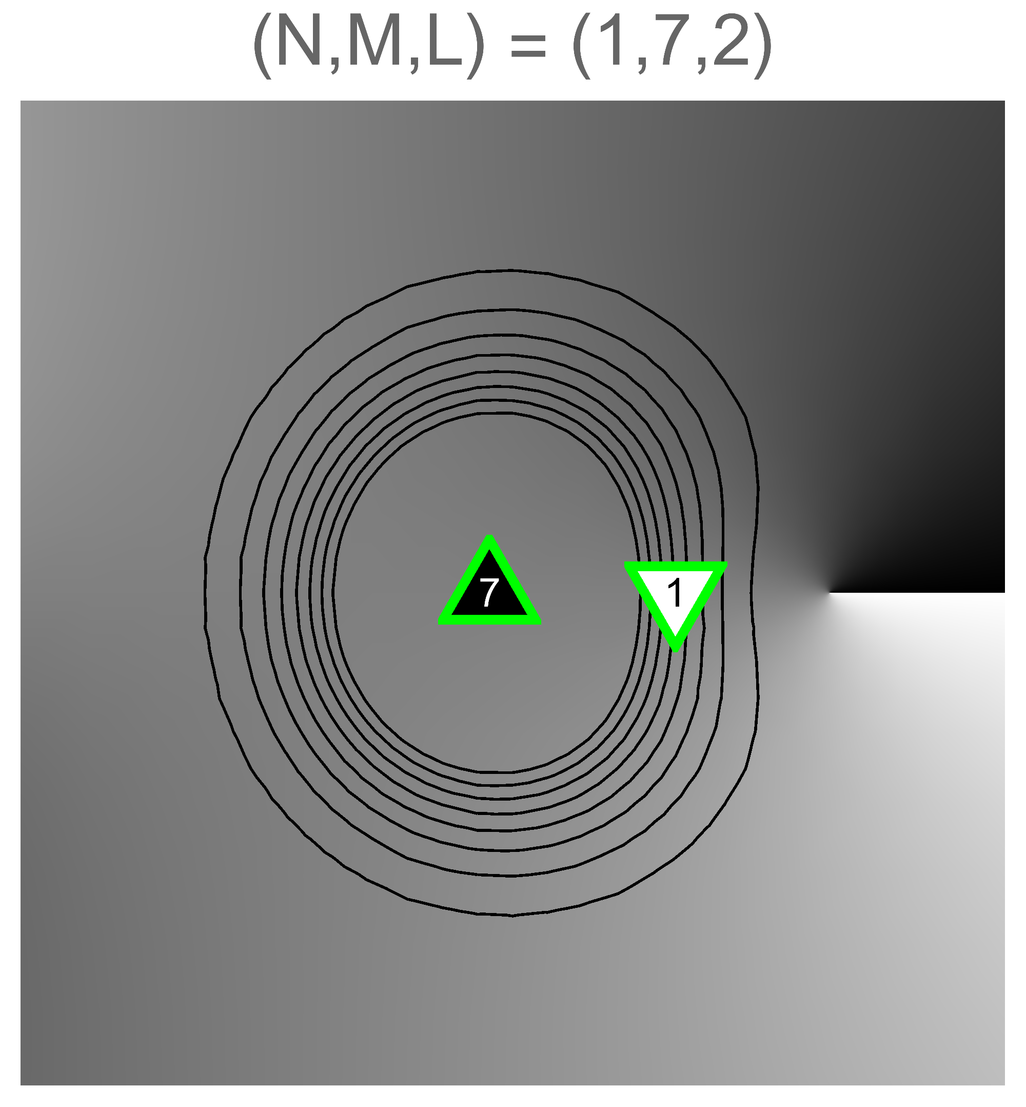 Figure 9
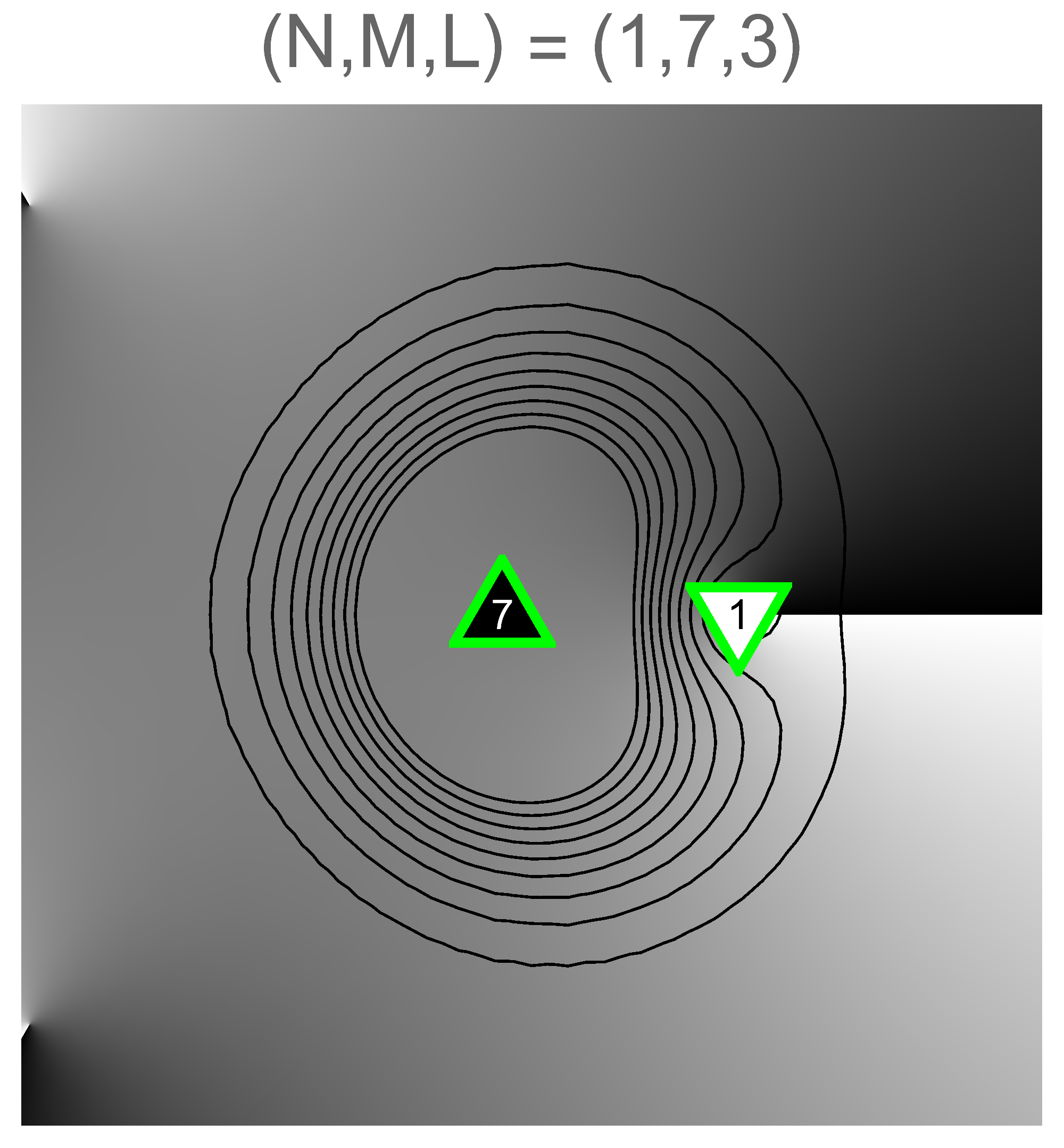 Figure 10
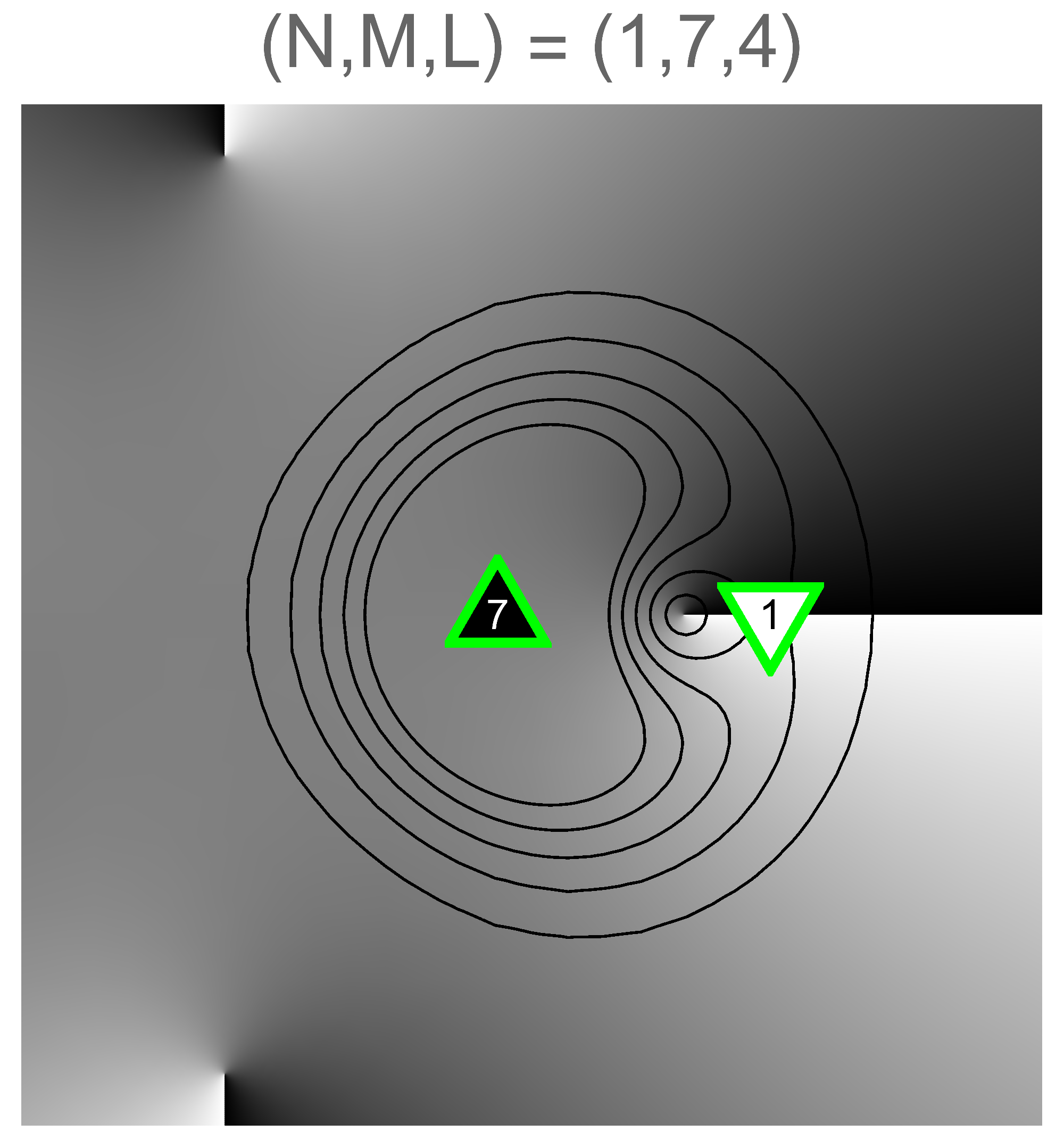 Figure 11
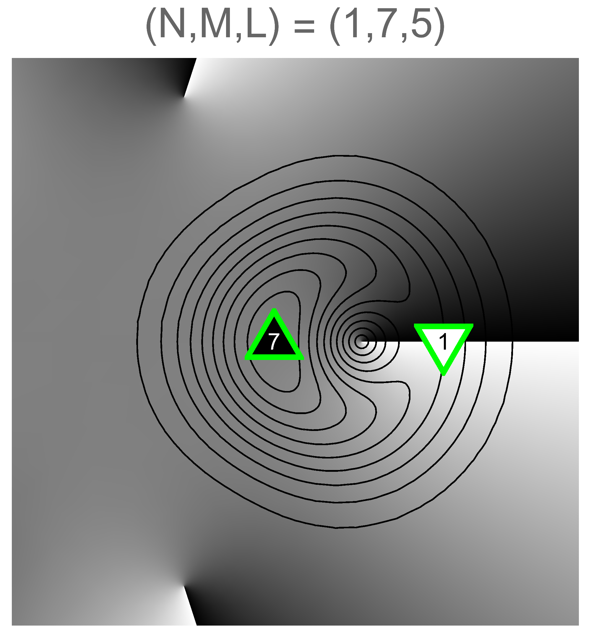 Figure 12
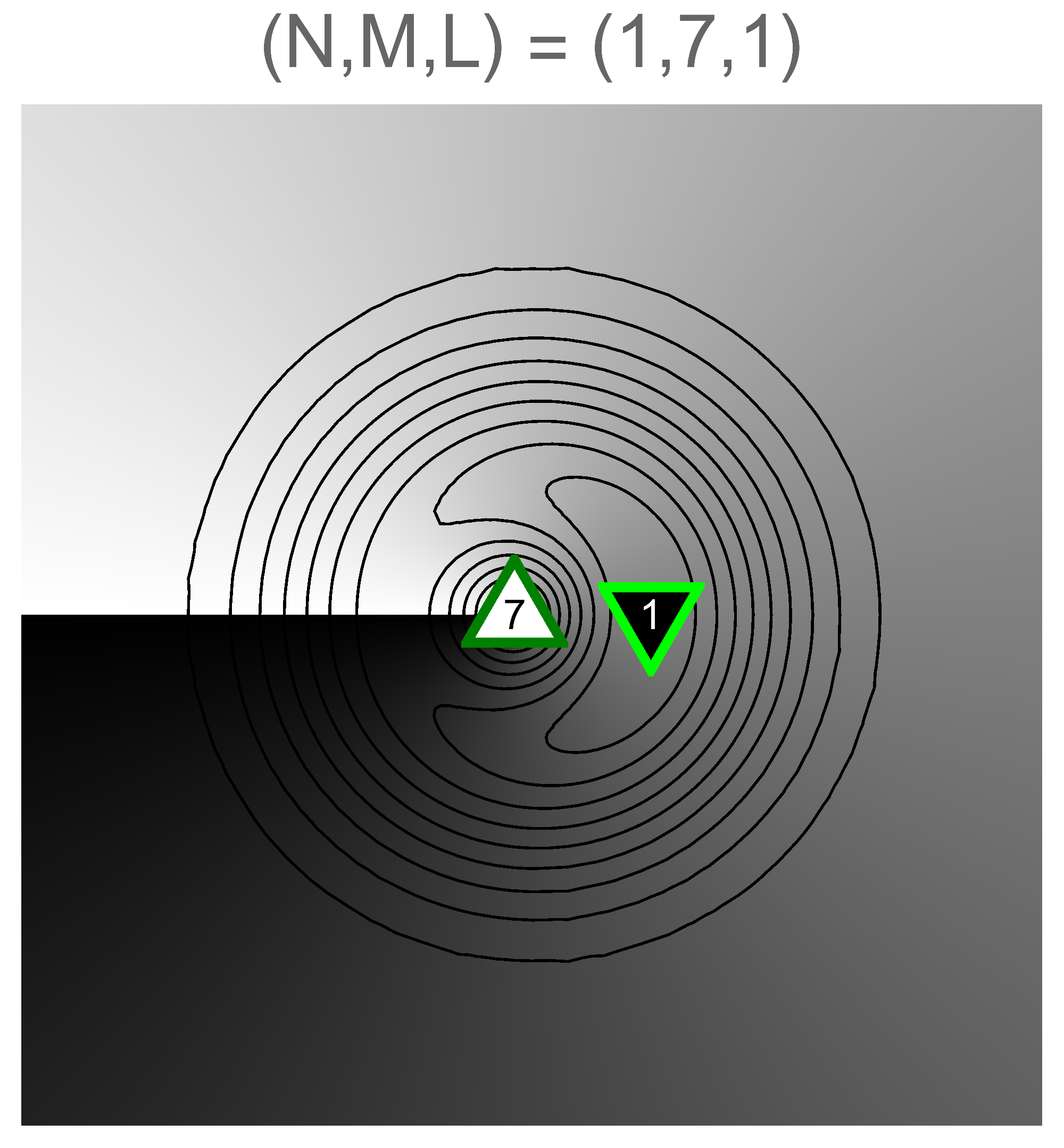 Figure 13
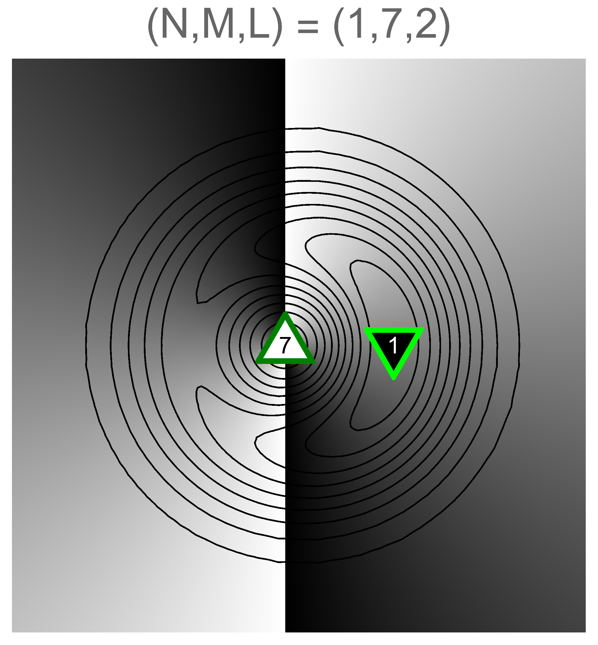 Figure 14
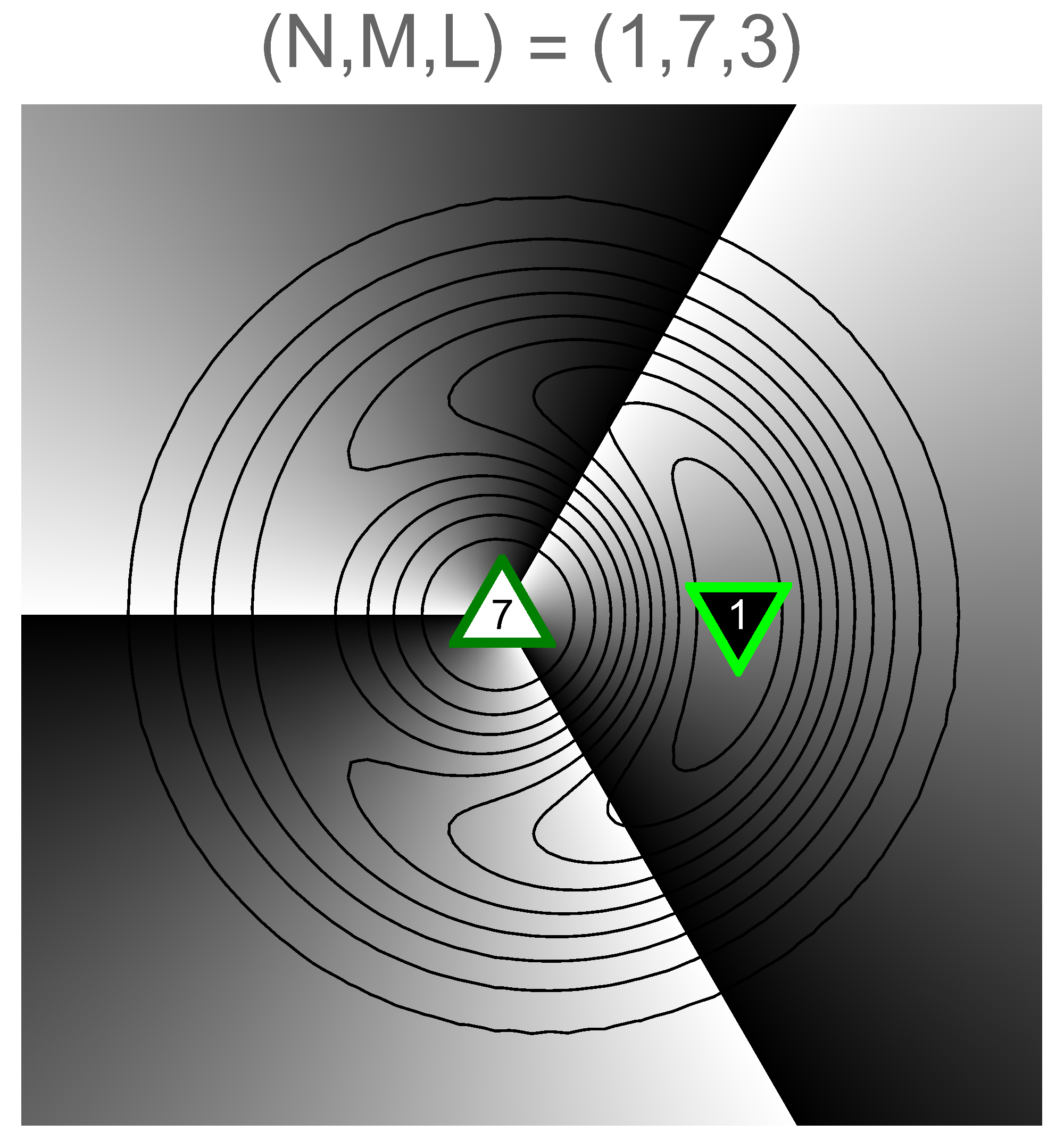 Figure 15
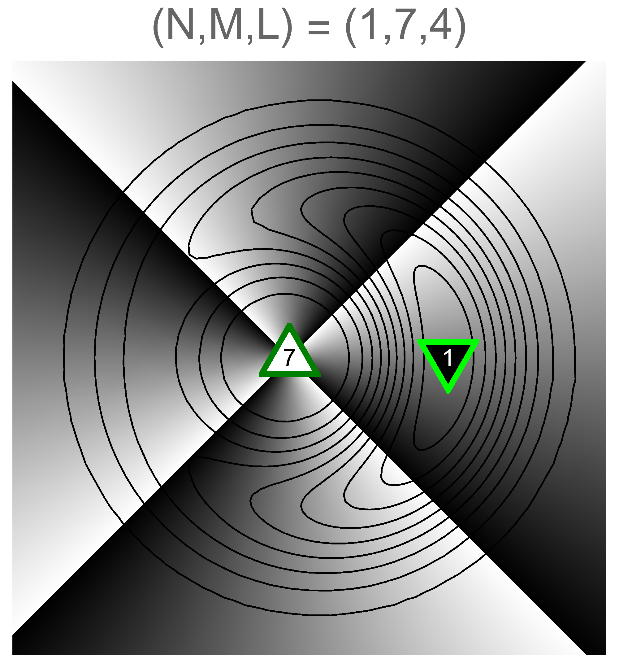 Figure 16
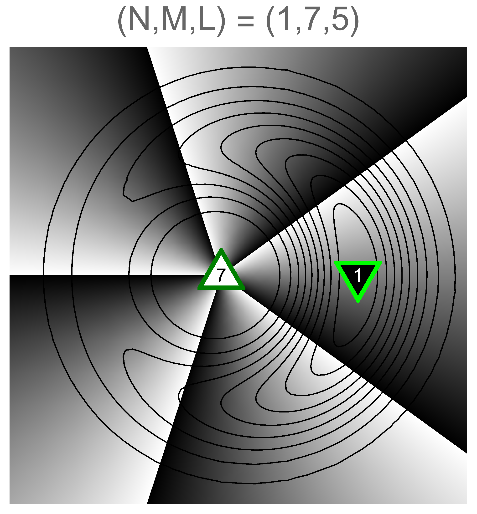 Figure 17
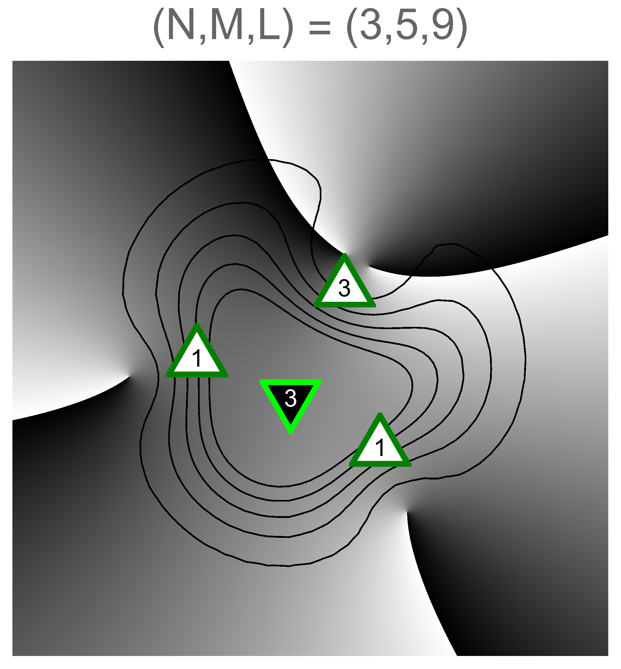 Figure 18
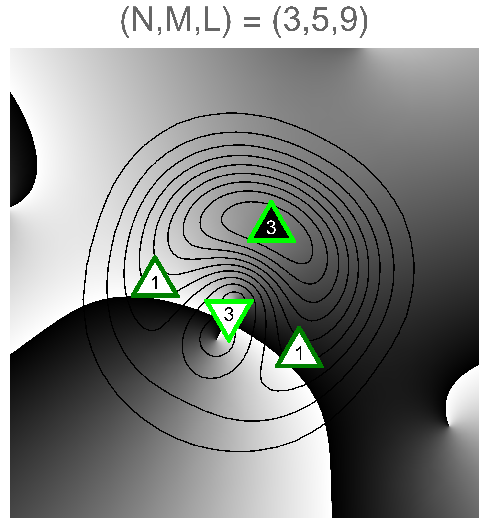 Figure 19
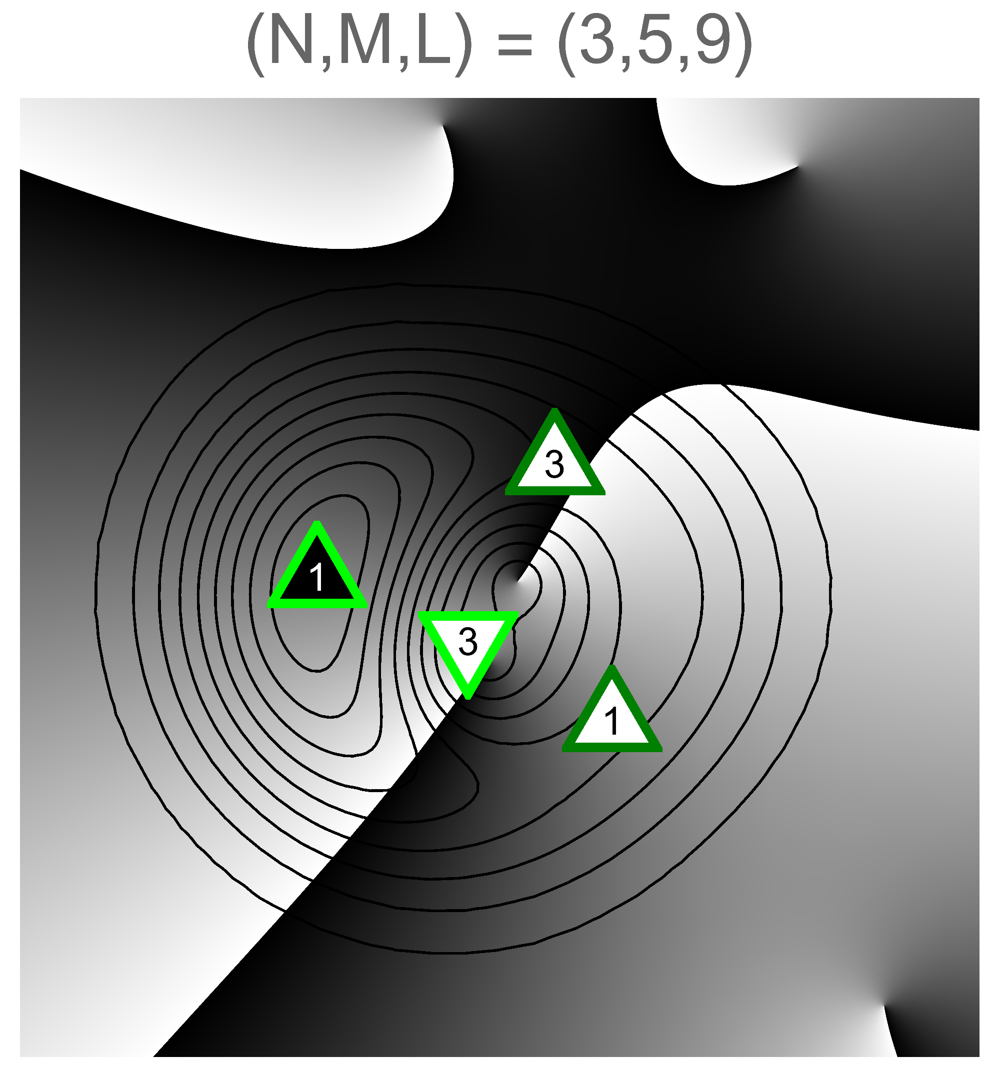 Figure 20
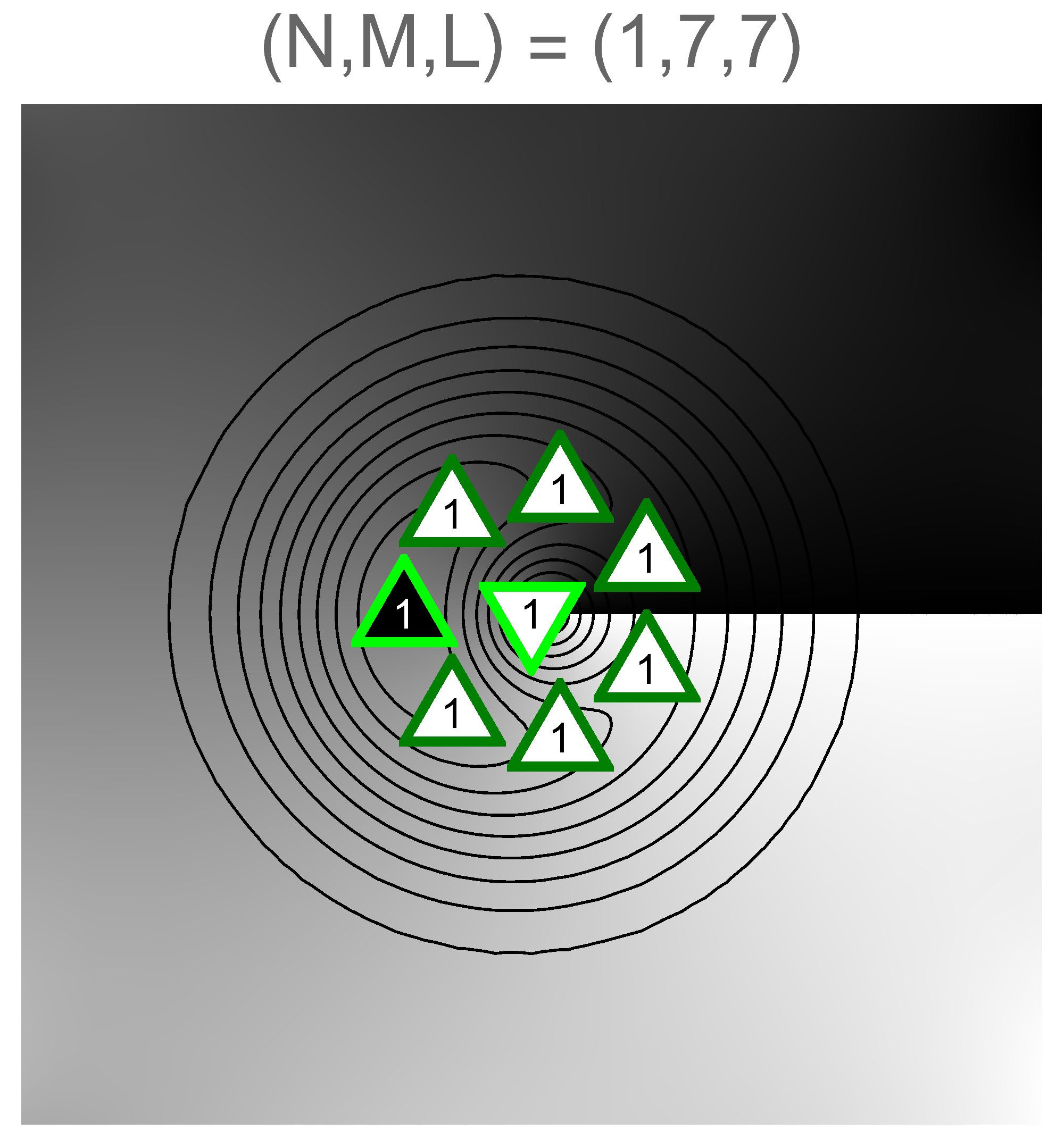 Figure 21
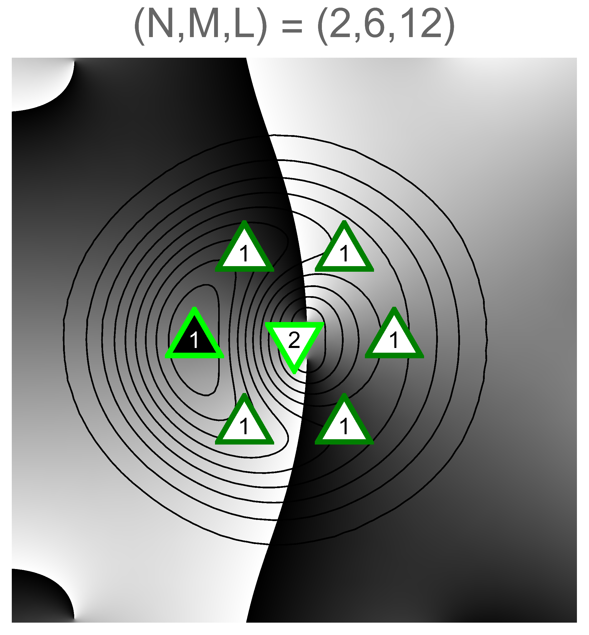 Figure 22
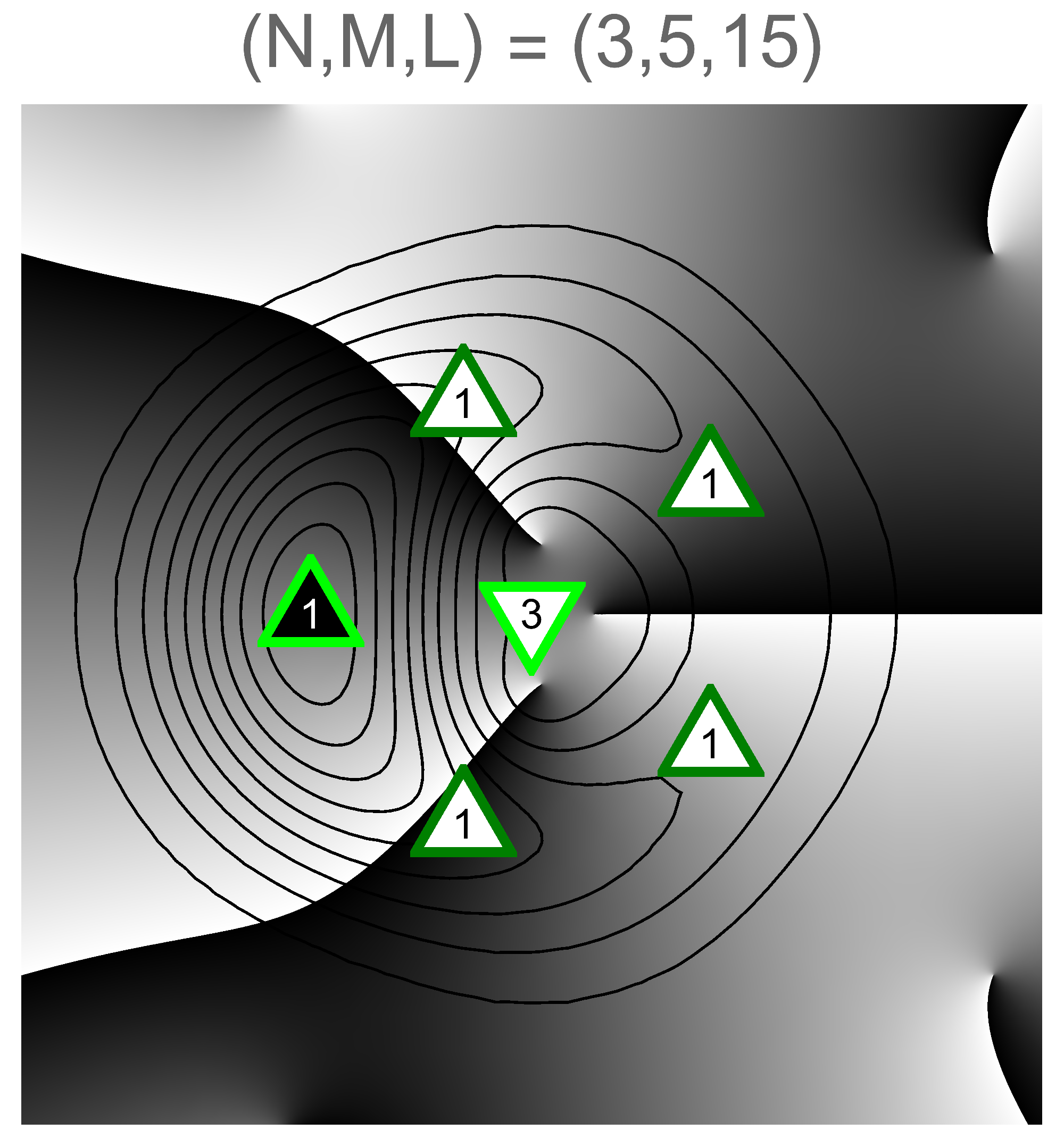 Figure 23
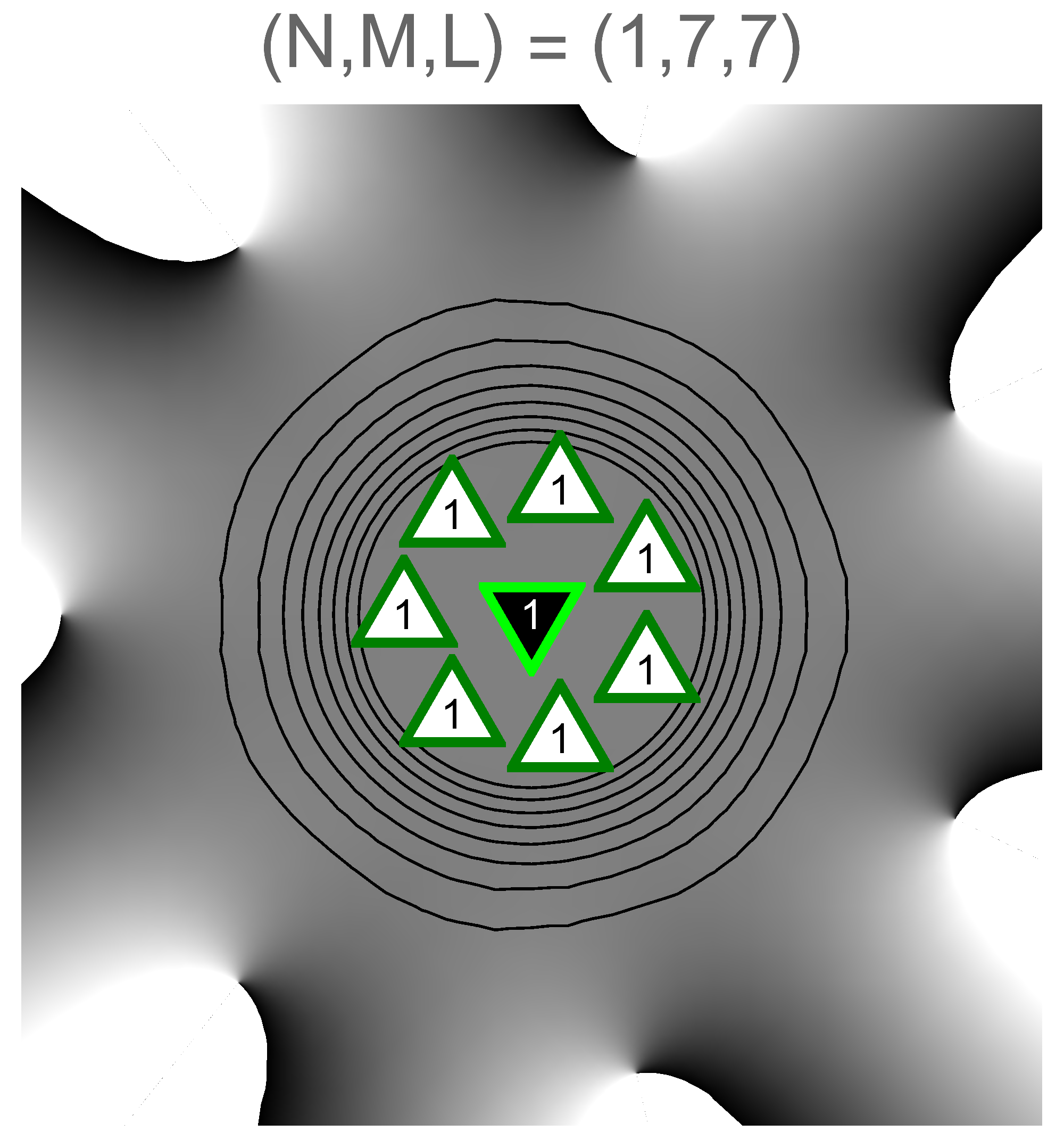 Figure 24
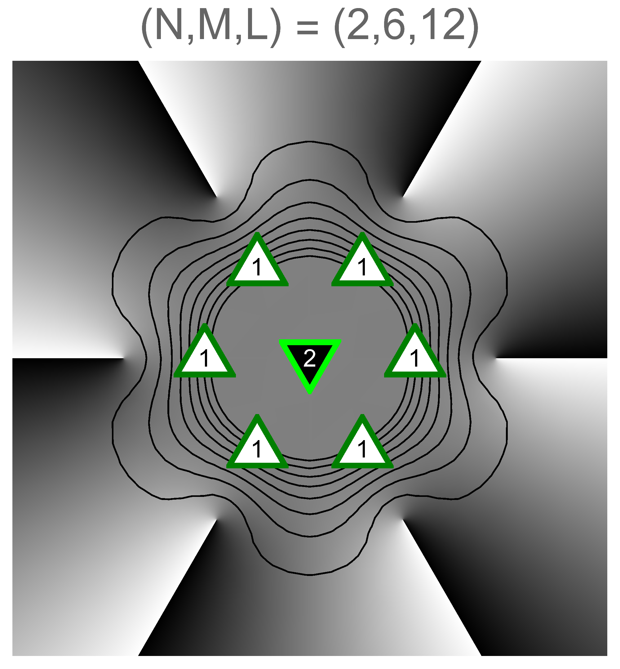 Figure 25
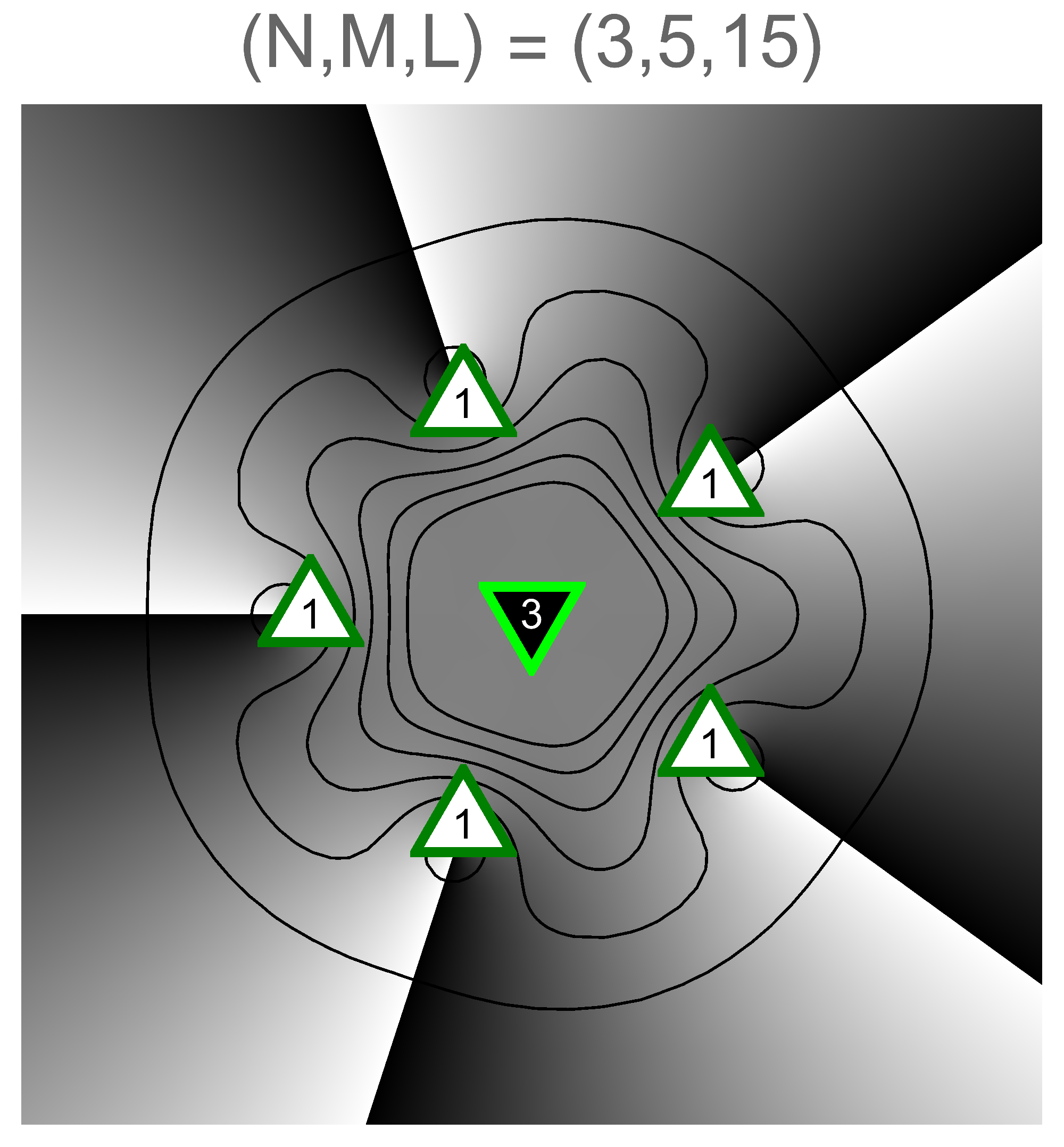 Figure 26
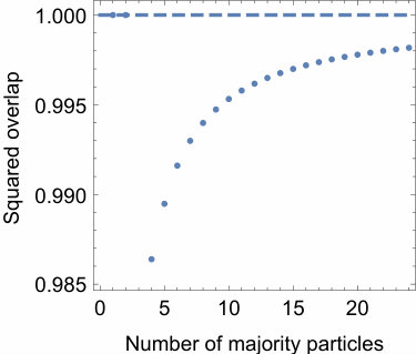 Figure 27
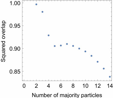 Figure 28
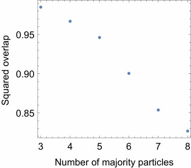 Figure 29
Peer Reviews
No public reviews on file for this paper yet. If you reviewed it on a platform where reviews are public (OpenReview, ICLR, NeurIPS, ICML), you can paste yours below so the community can read it here.
Videos
No videos yet. Explain this paper in a talk, walkthrough, or lecture? Add one.
Composite fermion basis for two-component Bose gases
O. Liabøtrø
M. L. Meyer
Department of Physics, University of Oslo, P.O. Box 1048 Blindern, 0316 Oslo, Norway
Abstract
Despite its success, the composite fermion (CF) construction possesses some mathematical features that have, until recently, not been fully understood. In particular, it is known to produce wave functions that are not necessarily orthogonal, or even linearly independent, after projection to the lowest Landau level. While this is usually not a problem in practice in the quantum Hall regime, we have previously shown that it presents a technical challenge for rotating Bose gases with low angular momentum. These are systems where the CF approach yields surprisingly good approximations to the exact eigenstates of weak short-range interactions, and so solving the problem of linearly dependent wave functions is of interest. It can also be useful for studying higher bands of fermionic quantum Hall states. Here we present several ways of constructing a basis for the space of so-called “simple” CF states for two-component rotating Bose gases in the lowest Landau level, and prove that they all give sets of linearly independent wave functions that span the space. Using this basis, we study the structure of the lowest-lying state using so-called restricted wave functions. We also examine the scaling of the overlap between the exact and CF wave functions at the maximal possible angular momentum for simple states.
pacs:
I Introduction
Almost 20 years ago, the connection between the physics of charged particles moving in two dimensions in a strong magnetic field, and dilute cold atoms rotating rapidly in a harmonic trap, was noticed wilkin-gunn-smith98 . Since then, a large body of theoretical and experimental work has accumulated that explore the various aspects of rapidly rotating atomic gases and the associated quantum phenomena; for reviews, see e.g. viefers-review ; cooper-review ; fetter-review . In particular, one expects strongly correlated phases similar to those found in the quantum Hall effect when the atoms experience strong synthetic magnetic fields. The effect of a synthetic magnetic field can be generated by simply rotating the cloud, or by more advanced techniques cornell04 ; roncaglia11 ; gemelke10 ; lin09 ; dalibardreview .
For electron systems, one prominent way of theoretically studying the quantum Hall effect involves constructing (classes of) explicit trial wave functions that approximate the true low-energy eigenstates of the interacting system. At least in the case of Coulomb interaction, the true many-body eigenstates are extremely complicated. Still, many successful trial wave functions exist, most famously the Laughlin wave functions laughlin83 , the family of composite fermion (CF) states jain89 , and trial wave functions addressing non-Abelian quantum Hall states moore91 ; read99 ; ardonne-schoutens99 . The success of these trial wave functions in explaining various phenomena is linked to the way they capture the important topological properties of the phases they describe.
Many of the methods mentioned above have been modified to be applicable to weakly interacting cold atom systems cooper-wilkin99 ; viefers00 . The hope is to be able to experimentally study strongly correlated states in a cold atom setting, where parameters like density, disorder and scattering lengths may be tuned much more finely than in the semiconductor systems traditionally used in quantum Hall experiments bloch08 . More recently, an additional degree of freedom is often taken into consideration in models and experiments, called pseudospin hall98 ; kasamatsu03 . Typically this means multicomponent mixtures where the different components are different internal states of the atoms. Varying inter- and intraspecies interactions independently allows for novel behaviours kasamatsu-tsubota-ueda05 . This pseudospin degree of freedom has been incorporated in the composite fermion scheme used for cold atom systems, and has been used in the quantum Hall regime of high angular momenta jain13 ; grass14 . On the other hand, near the lower end of the angular momentum scale, where the CF description is not a priori expected to work, it has been shown that it actually works surprisingly well, both in scalar and two-component cases korslund06 ; meyer14 .
A property of the CF method of constructing wave functions is that one typically needs to do a projection into the lowest Landau level (LLL) in order to either compare different CF wave functions, or to compare a CF to an eigenstate found by numerical diagonalization of the interacting Hamiltonian jainbook . This projection leads to non-orthogonal, and often also linearly dependent, CF wave functions. This has been known in the context of electrons in the quantum Hall regime dev-jain92 ; wu95 ; balram13 , but the issue is much more prominent for bosons with low angular momentum: we have previously observed meyer-lia16 one or two orders of magnitude difference between the number of seemingly distinct CF candidates and the actual number of linearly independent wave functions. In some extreme cases the number of seemingly distinct CF candidates one can write down is even larger than the dimension of the relevant sector of Hilbert space, meaning they cannot possibly be independent. Until very recently, little was understood about the mechanisms responsible for these linear dependencies after projection. In a previous paper meyer-lia16 , we discussed three types of relations between certain types of low-lying CF candidates, but were only able to give examples demonstrating how these relations seem to explain all the linear dependencies.
In this paper, we present sets of CF candidates for two-component systems that we rigorously prove are basis sets for the subspace that minimizes the CF cyclotron energy for low angular momenta. We use these states to study the real-space distribution of particles and vortices of the lowest-lying wave functions when we vary the angular momentum, and also give additional attention to certain special cases, comparing to known behaviour from scalar gases.
II Two-component rotating Bose gases
We first summarize the model for two-species Bose gases in the lowest Landau level, including their description in terms of composite fermions. A more detailed introduction can be found in meyer14 . The two species of bosons experience a two-dimensional harmonic trap potential of strength , and are rotating about the minimum of the potential at frequency . The Hamiltonian is:
[TABLE]
Here denotes the number of particles of the minority species, and denotes the number of particles of the majority species, all with the same mass . is the angular momentum of particle . The strength of the contact interaction depends only on the species of particles . In the species-independent case constant, the system posesses a pseudospin-1/2 symmetry, which we will assume here. For sufficiently dilute gases, i.e. in the weak interaction limit, this reduces to the well known lowest Landau level problem viefers-review ; cooper-review in the effective magnetic field ,
[TABLE]
In the ideal limit the Landau levels become flat, meaning that the many-body eigenstates are solely determined by the interaction. Here are the dimensionless complex positions of the particles in units of the “magnetic” length . We name the coordinates of the two components , and , . Working in symmetric gauge, the single particle eigenstates in the lowest Landau level with angular momentum are
[TABLE]
The Gaussian factors are ubiquitous, so we suppress them for simplicity from now on. Since the Hamiltonian commutes with the total angular momentum , we may work with many-body wave functions that are eigenstates of . These are homogeneous polynomials of degree , symmetric in the coordinates of each species separately. As is common viefers-review ; meyer14 we will focus on translationally invariant states, i.e. polynomials invariant under a constant shift of all coordinates,
[TABLE]
As mentioned in the introduction, one may adapt the CF approach to produce wave functions for 2D bosons, both in the scalar and multi-component cases. A CF trial wave function for the bosonic two-species system is of the form jainbook
[TABLE]
where is an odd number, . , are Slater determinants for each species of CFs, treated as non-interacting to lowest order. They consist of CF orbitals
[TABLE]
where is the associated Laguerre polynomial, and is a normalization factor. The interpretation of these orbitals is that they are composite fermions occupying Landau-like levels, labeled by (often called -levels) in a reduced effective magnetic field. is a Jastrow factor involving both species,
[TABLE]
has units of angular momentum per pair of particles, in total . We will be considering low total angular momentum, hence we will choose the smallest possibility . denotes projection to the lowest Landau level. We use the projection of Girvin and Jach girvin-jach84 (called Method I in jainbook ), which amounts to first moving the conjugate variables to the left of the , and then replacing by .
In this paper, we focus on low angular momenta, specifically . We consider the set of translationally invariant CF wave functions that minimize the total CF cyclotron energy in this range. The sum runs over the CF orbitals occupied in a pair of Slater determinants. Since , we see that must be negative. We have previously shown that this set is spanned by CF candidates where only the orbitals are occupied, and that linear combinations of candidates in this set give good overlaps with the very lowest-lying states in the exact yrast spectrum meyer14 . After projection to the LLL, the orbitals become . This simple form of the Slater determinants has led these CF wave functions to be called simple states. Since the differential operators commute, we may perform the projection to the LLL on the Slater determinants individually, as long as we keep them to the left of the Jastrow factor. This is understood in the following sections.
III Composite fermion basis
We now present some sets of states that we prove to be bases for the space of simple states with particles and angular momentum . First, we need some definitions. The simple states are on the form (5), where the Slater determinants after projection are
[TABLE]
and
[TABLE]
with . In the following, we will focus on , but we will never use that , so replacing is always possible.
We define
[TABLE]
This is the set of partitions of into an box. We order the partitions lexicographically. The partitions can be visualized using Young diagrams. Such a diagram is obtained by coloring cells of an box compactly from the lower left. The number of colored cells in the lowest row is , the next row corresponds to , and so on. As an example, we show all the Young diagrams corresponding to the set in FIG. 1.
There is a one to one correspondence between and given by
[TABLE]
We define the following differentiation operators:
[TABLE]
and
[TABLE]
We have that
[TABLE]
and
[TABLE]
The maximal state occurs when the Slater determinants contain minimal differentiation operators, i.e.
[TABLE]
where . We will continue to use the vectors and as they are useful not only for but also for general . We can now state our main theorem:
Theorem 1**.**
The sets
[TABLE]
are bases for the set of simple CF states with particles and angular momentum . The sets and are also bases.
In fact, for even. Otherwise, the sets contain times the vectors of the other. This can be seen as a consequence of reflection symmetry, as introduced in meyer-lia16 .
Proof.
We first show that spans ; we already know from Eq. (14) that spans . We then show that spans the set of simple CF states, and finally that is a linearly independent set. This must also hold for since . We refer to lemmas that we prove in the appendix.
Lemma 1 states that spans :
[TABLE]
for coefficients , where . The lemma also shows that we can write a general simple CF state as
[TABLE]
Lemma 2 states that we can write
[TABLE]
with coefficients . We can therefore write
[TABLE]
Next, we can apply generalized translation invariance (Lemma 3),
[TABLE]
to replace the operators with , giving
[TABLE]
where is if there is an odd number of that are non-zero, and otherwise.
We can see from eqs. (14, 15) that this gives terms that are all on the form for varying . We have now expressed a general simple state as a linear combination of elements of , and the same can be done for . All that remains is to show that is a linearly independent set, and this result is Lemma 4. ∎
To summarize, we have now shown that either of the sets (Eq. (17) ) are basis sets for the simple CF wave functions at angular momentum . In other words, when constructing basis sets for simple states, we can always fix () to () and then vary the () determinant. The number of ways to do that, i.e. the size of the basis, is simply . We plot this as function of for in FIG. 2. The symmetry of each curve about its midpoint that was originally observed in meyer-lia16 is now easily understood because the number of ways to color cells in a Young diagram leaves cells uncolored, meaning that the diagrams are 1-1 with the diagrams. We have illustrated this in FIG. 3.
IV Structure of the lowest-lying wave functions
Using the simple CF basis sets presented in the previous section, we can now diagonalize the interaction Hamiltonian in the simple CF subspace, to produce approximations to the lowest-lying wave functions of the two-component rotating gas. Because the size of the simple CF basis is so much smaller than the size of the Hilbert space, this is often a huge computational simplification. We now take advantage of this to study some aspects of these low-lying states.
In order to increase our physical understanding of the structure of these states, one option is to study density and pair correlation functions. Another approach that is particularly suitable to visualizing vortex structure is to compute the so-called restricted wave function (RWF) rwf-1 ; rwf-2 . To find the RWF of a given many-body wave function , one first calculates a set of particle coordinates that maximises . The restricted wave function is defined as
[TABLE]
We see that this function varies as one of the particles is allowed to move from its maximizing position. The amplitude of gives the relative amplitude of the many-body wave function compared to the maximum, and the argument gives the change in phase. The vortices can be identified from plots of where the nodes of the amplitude meet lines where the phase jumps.
An example of an RWF plot is shown in FIG. 4. The wave function in this example is the exact ground state for a single-species gas with 8 particles at . For a single component, the cases are known as single vortex states korslund06 ; vortex-review . The triangular plot markers show the optimal positions . The number on each plot marker specifies how many particles share that position. The plot marker with black filling corresponds to the particle whose position is varied in the plot. The contour lines show lines of constant amplitude of and the color shows the phase change, where black corresponds to and white to . In this case, the configuration of highest is a ring of particles, with a vortex clearly visible close to the center of the ring.
In our two-component case, we can define an RWF for each species, and for minority and majority species respectively. The difference is simply the species of the particle whose position we vary. We will use triangles pointing down as plot markers for the minority component particles, and triangles pointing up for majority particles (like and , respectively).
In FIG. 5 we see that there is a substantial difference between the RWF plots and . In the top row we see a vortex approaching the cloud from the side where the lone minority particle is located, starting far outside the cloud and coming closer and closer to the center as increases. On the other hand, the lone minority particle sees a vortex coinciding with the lump of majority particles already at , a so-called coreless vortex kasamatsu-tsubota-ueda05 ; christensson08 . This is consistent with findings using full diagonalization bargi07 . The multiplicity of this vortex increases with , and the vortex and majority particles move together, away from the lone minority particle. This displays an example of how the “perspectives” of the two species can be very different for a given state . A similar pattern is also observed for for .
For , a variety of configurations are realized as those maximizing . The common features are that, as increases and the particles spread out more, particles of the same species still tend to stay close to or on top of some of the other ones, rather than all of them spreading out. The vortices are exclusively located near the particles of the opposite species: no same-species nodes are observed for the we consider. Finally, the mean number of phase jump lines per particle of the opposite species increases with . A more or less typical situation is shown in FIG. 6. The majority species has split into three groups, but three of them are still close together. The minority particles are all in the same position. In both (b) and (c), there are two nodes close to the lump of three minority particles. Since the only difference between (b) and (c) is which majority particle coordinate we choose to vary, this demonstrates that the vortex configuration that is seen is not sensitive to that choice, which is what we would expect of a physical vortex state.
Finally we discuss the maximally rotating simple states, namely the states in Eq. (16). For a given this is the only possible simple state at , i.e. no CF diagonalization is necessary. The restricted wave functions of some states are shown in FIG. 7. Again we see a very clear distinction between minority and majority species particles. The majority particles are positioned on the vertices of a regular -gon, with all the minority particles in the center. In (a) - (c) we see what looks like a single, double and triple vortex structure, respectively, but filled by the minority component. The qualitative behaviour of the amplitude contours is largely the same in the three plots. In particular, 7(a) looks remarkably similar to FIG. 4 except for the minority particle in the middle. We will come back to this point in SEC. V.
It can be noted that, while the single vortex for a scalar gas appears at , the general multiply quantized vortex of winding appears at ; for 20 particles, the double and triple vortices appear at 1.8 and 2.85 respectively vortex-review . The results presented here seem to indicate that the vortex of winding appears at , but that the vortex is a coreless vortex in the majority component. On the other hand, (d) - (f) show how evolves from a more or less Gaussian distribution in (d) to a situation where one node radially approaches each majority particle from outside the cloud.
V Overlaps
When working with trial wave functions like CF wave functions, especially in a context for which CF was not originally intended, like the slowly rotating Bose systems we are discussing, one should carefully compare the results obtained with ones obtained by other means. In the lowest Landau level, we are fortunate because the Hilbert space of each sector is finite. Given enough computer resources, one can therefore in principle compute the exact spectrum (at least to machine precision) for a given , and compare the CF results to this. In practice, desktop computers can handle two-component systems with up to a total of around 15-20 particles for the considered in this paper. This method has been used to verify the applicability of the CF construction to scalar cooper-wilkin99 ; korslund06 and two-component systems both below and in the quantum Hall regime grass14 ; jain13 ; meyer14 .
In particular, korslund06 ; viefers10 showed that the overlap between the exact and CF state for the scalar case (the single vortex) increases to unity in the limit. As mentioned in the previous section, this is the state plotted in FIG. 4 for . It strikingly resembles the restricted wave function plot of the state with a single minority particle, FIG. 7. This resemblance, and the fact that the state is unique for given , led us to compute the overlap between the exact lowest-lying state and the CF state as function of for given .
In FIG. 8, the squared overlaps between the maximally rotating simple CF wave functions at and the exact lowest-lying states are plottet as functions of for in (a) - (c) respectively. In (a), we see exactly the same convergence to unity as was reported in korslund06 ; viefers10 for one component. The CF candidate in the one-component case is not simple (simple states don’t exist in the scalar case), but it is unique and minimizes the CF cyclotron energy. The exact ground state of the single vortex, on the other hand, is known, and its polynomial part is simply proportional to
[TABLE]
where are the particle coordinates relative to the center of mass, and is the elementary symmetric polynomial of degree . In fact, for , the exact lowest-lying state is known also in the two-component case: it was given in pap-rei-kavo12 and its polynomial part is proportional to
[TABLE]
Here are the particle coordinates relative to the center of mass for all particles.
In (b) and (c) however, we clearly see that the squared overlap decreases with system size, as is usually the case with most trial wave function approaches. It should be stressed that the dimension of the relevant sector of Hilbert space grows very rapidly with system size, so given that is a unique state in this space, it is still surprising that the overlap with the true lowest-lying state is as large as it is. We should also remember that we have restricted ourselves to simple states in this analysis: the fact that the overlap decreases with system size therefore tells us that higher bands of CF cyclotron energy contribute significantly for larger systems.
VI Conclusions and outlook
The main results of this paper are the identification of basis sets of simple CF states, and the proof that these sets are in fact spanning the simple state subspace and are linearly independent. We have used these basis sets to revisit the spatial structure of particles and vortices for the rotating two-component Bose gas in the LLL at low angular momenta, and have paid special attention to the unique simple CF candidates at angular momentum . We find that for minority particle, the system mimics the CF candidate for the single vortex state of the scalar rotating gas. This includes an overlap with the exact wave function that converges to 1 in the limit. For , we observe a coreless vortex of winding in the majority species at exactly . From the plots in FIG. 8, however, we see that the exact wave function must have contributions from CF states in higher bands. To answer whether or not this makes any qualitative differences from the results presented here would require further investigation.
As presented in meyer-lia16 , there are still linear dependence relations between CF candidates in higher bands that are not understood. However, now that we have a good understanding of the relations for simple states, it might be possible to make further progress for these so-called “compact states” jainbook . They are the relevant candidates for in the system studied here, but they are also relevant for electrons in strong magnetic fields, confined to quantum dots jain-kawamura95 .
For other projection methods jainkam97a and/or geometries haldane83 , we expect some linear dependence relations similar to the ones in this paper. The reason is that, as we have seen, it is in fact the Jastrow factor that is responsible for the equations that relate different -level configuration patterns. Certainly some rules will need to be modified, but the principle of translation invariance should still hold.
Acknowledgement
We would like to thank Susanne Viefers for helpful comments on the manuscript. This work was financially supported by the Research Council of Norway.
Appendix A Mathematical results
Lemma 1**.**
There exists such that
[TABLE]
*where . .
Proof.
We use the one to one correspondence between the elements of and given by
[TABLE]
and induce an ordering on the Slater determinants such that
[TABLE]
We have that
[TABLE]
The non-zero terms are all Slater determinants. The greatest determinant with respect to the ordering occurs when orders the partition non-decreasingly. This particular determinant is and we may therefore write
[TABLE]
for some integers . It is important that
[TABLE]
It is in fact positive, since every permutation that gives this determinant leaves the elements of in increasing order. It follows that for the smallest partition, , we have
[TABLE]
and in general
[TABLE]
Eq. (33) says that the Lemma holds for and eq. (34) says that it holds for if it holds for all . It must therefore hold for all . ∎
Lemma 2**.**
For all , there exists such that
[TABLE]
where we define .
Proof.
Our proof is based on induction. We first define the subset
[TABLE]
and note that trivially, for all , there exists such that eq. (35) holds. There is only one such p and . Now, we assume as induction hypothesis that (35) holds for all when .
Let and consider the polynomial
[TABLE]
It is a product of factors. Each factor is a sum of differentiation operators with respect to different variables. The resulting terms with the highest number of non-zero exponents are those that do not multiply differentiation operators for the same variable from several different factors . This is except for the last as and any of the combinations gives the same. This restricted part of can be described by permutations as
[TABLE]
and this means that
[TABLE]
where is a polynomial of differentiation operators where each term has at most non-zero exponents. By the induction hypothesis, these can all be written on the form (35). This implies that the hypothesis is also true for all and completes the proof. ∎
As was introduced in meyer-lia16 , the simple CF states obey
Lemma 3** (Generalized translation invariance).**
[TABLE]
for all integers .
Ordinary translation invariance is captured in the case .
Proof.
The operator commutes with the Slater determinants, so it is enough to show that . This result is independent of the splitting of particles into and type. We can therefore use variables . We have that
[TABLE]
Now, for each pair , there is a unique pair such that and and for all . Since and only differ by a permutation of two elements, and the corresponding terms in eq. (41) cancel out. Since this happens for all , it follows that . ∎
Lemma 4** (Linear independence).**
[TABLE]
is a linearly independent set.
Proof.
If
[TABLE]
then we denote the projection onto by , and the set of projected states by . We will show that this set is linearly independent and therefore is as well.
The -independent terms of arise when the operators act on the lowest order variables in the Jastrow factor. We can therefore write
[TABLE]
We are interested in the particular symmetrized term that occurs when is the identity operator. We name this term , and it can be written as
[TABLE]
where is an integer that results from differentiation and possibly a permutation sign. The term has the property that the smallest exponent is as great as possible among terms in . Given that, the second smallest exponent is as great as possible and so on. We use this to define an ordering on the terms, saying that
[TABLE]
iff the ’th least exponent of is greater than the ’th least exponent of and their least exponents are pairwise equal. This is equivalent to , and if we pick another non-zero term of by choosing a that is not the identity, then we have . We index the partitions such that
[TABLE]
Now, if , then . This means that contains a polynomial term that is not contained in any for all . This means that if there exists a linear dependence relation
[TABLE]
then the leftmost non-zero coefficient of this relation must be 0, and the relation must therefore be trivial. ∎
The reference list from the paper itself. Each links out to its DOI / PubMed record.
- 1(1) N.K. Wilkin, J.M.F. Gunn, and R.A. Smith, Phys. Rev. Lett. 80 , 2265 (1998).
- 2(2) S. Viefers, J. Phys.: Cond. Mat. 20 , 123202 (2008).
- 3(3) N. Cooper, Advances in Physics 57 , 539 (2008).
- 4(4) A. L. Fetter, Rev. Mod. Phys. 81 , 647 (2009)
- 5(5) V. Schweikhard, I. Coddington, P. Engels, V. P. Mogendorff, and E. A. Cornell, Phys. Rev. Lett. 92 , 040404 (2004).
- 6(6) M. Roncaglia, M. Rizzi, and J. Dalibard, www.nature.com, Scientific Reports 1 , doi:10.1038/srep 00043 (2011).
- 7(7) N. Gemelke, E. Sarajlic, and S. Chu, ar Xiv:1007.2677.
- 8(8) Y.-J. Lin, R. L. Compton, K. Jiménez-García, J. V. Porto, and I. B. Spielman, Nature 462 , 628 (2009).