Statistical analysis of the first passage path ensemble of jump processes
Max von Kleist, Christof Sch\"utte, Wei Zhang

TL;DR
This paper develops a statistical framework for analyzing the first passage paths of jump processes, including non-ergodic and non-Markovian cases, with algorithms for practical computation and applications across various fields.
Contribution
It introduces a novel approach to decompose first passage paths into segments and provides algorithms for their statistical analysis, applicable to a broad class of jump processes.
Findings
Applicable to non-ergodic jump processes
Provides efficient algorithms for path statistics
Links first passage analysis with transition path theory
Abstract
The transition mechanism of jump processes between two different subsets in state space reveals important dynamical information of the processes and therefore has attracted considerable attention in the past years. In this paper, we study the first passage path ensemble of both discrete-time and continuous-time jump processes on a finite state space. The main approach is to divide each first passage path into nonreactive and reactive segments and to study them separately. The analysis can be applied to jump processes which are non-ergodic, as well as continuous-time jump processes where the waiting time distributions are non-exponential. In the particular case that the jump processes are both Markovian and ergodic, our analysis elucidates the relations between the study of the first passage paths and the study of the transition paths in transition path theory. We provide algorithms to…
Click any figure to enlarge with its caption.
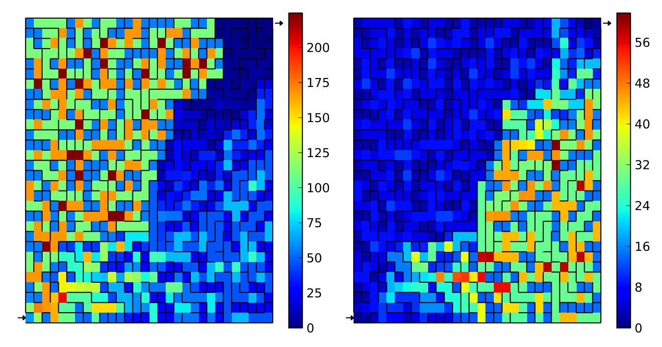 Figure 1
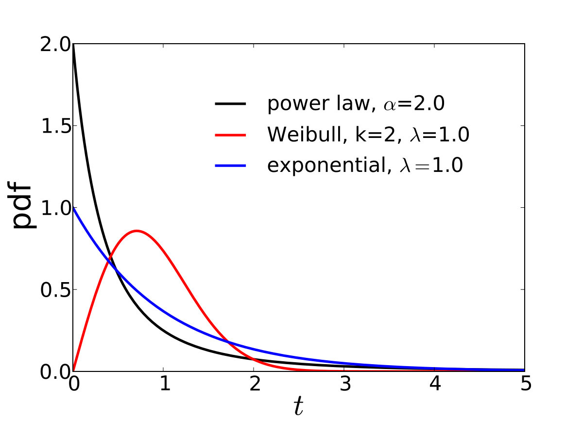 Figure 2
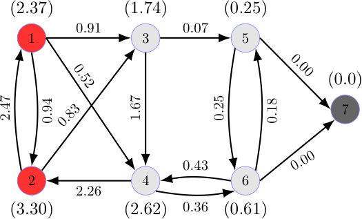 Figure 3
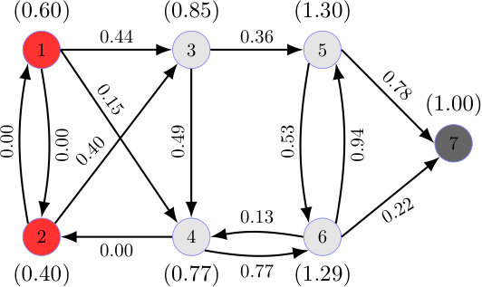 Figure 4
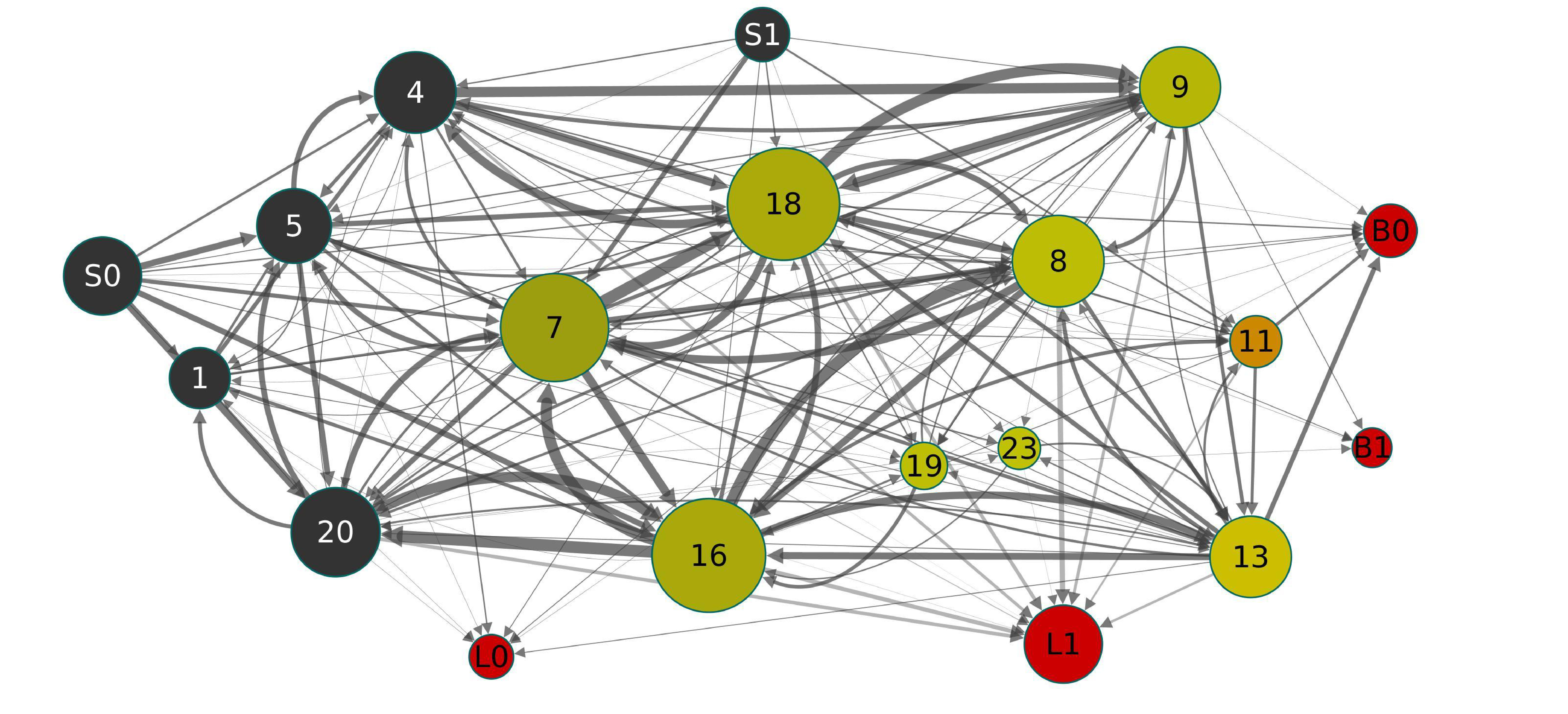 Figure 5
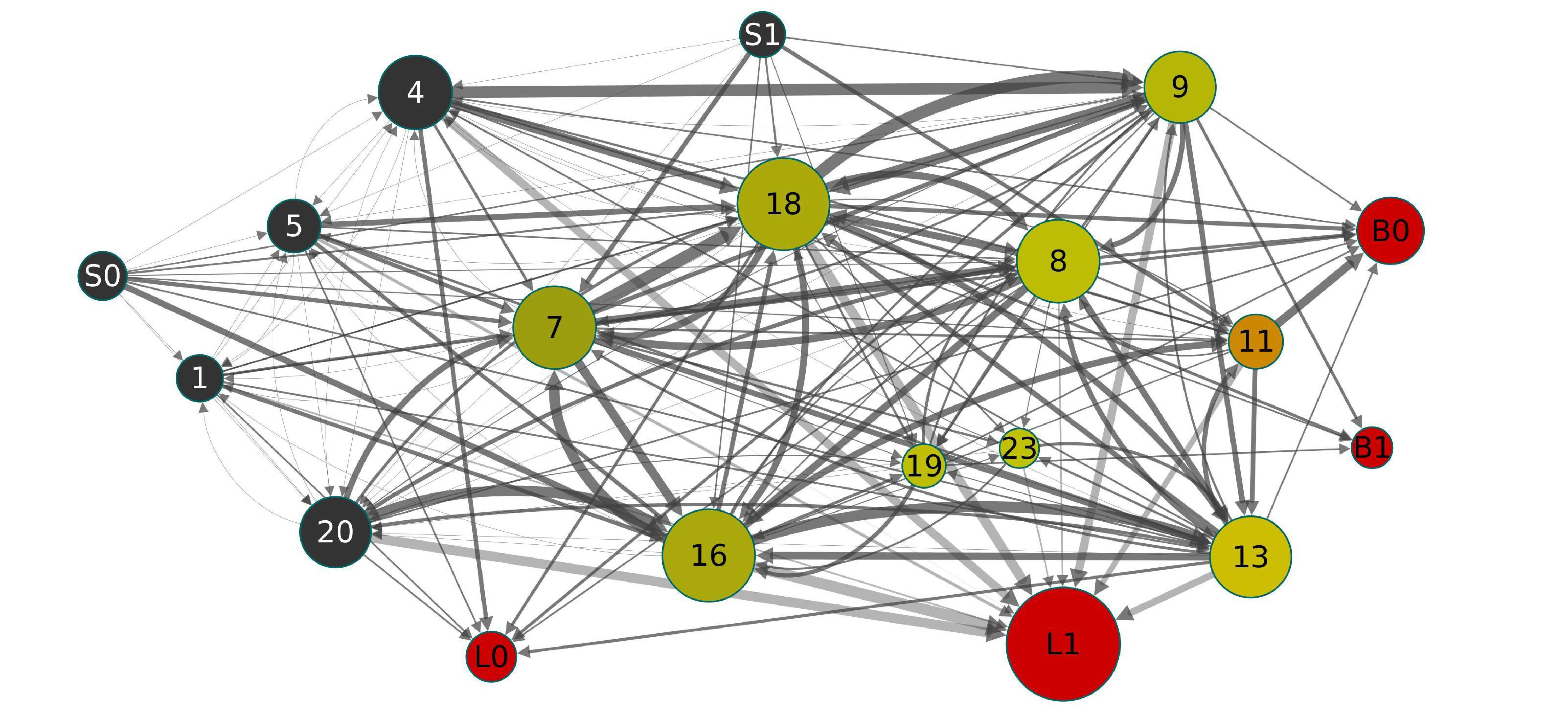 Figure 6
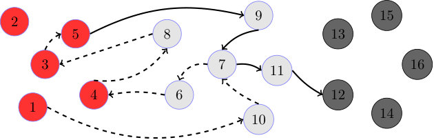 Figure 7
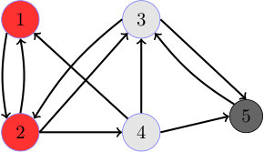 Figure 8
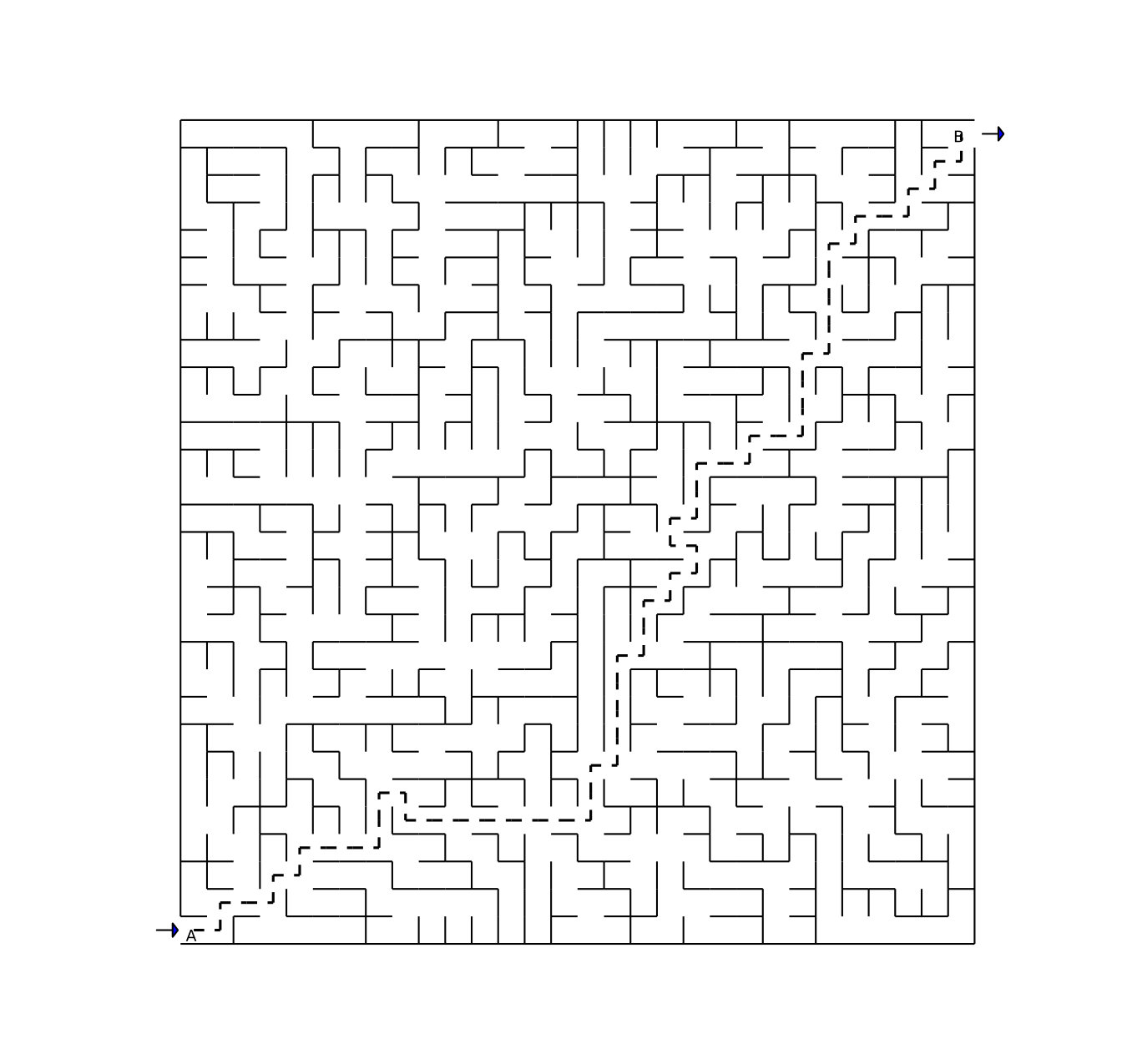 Figure 9
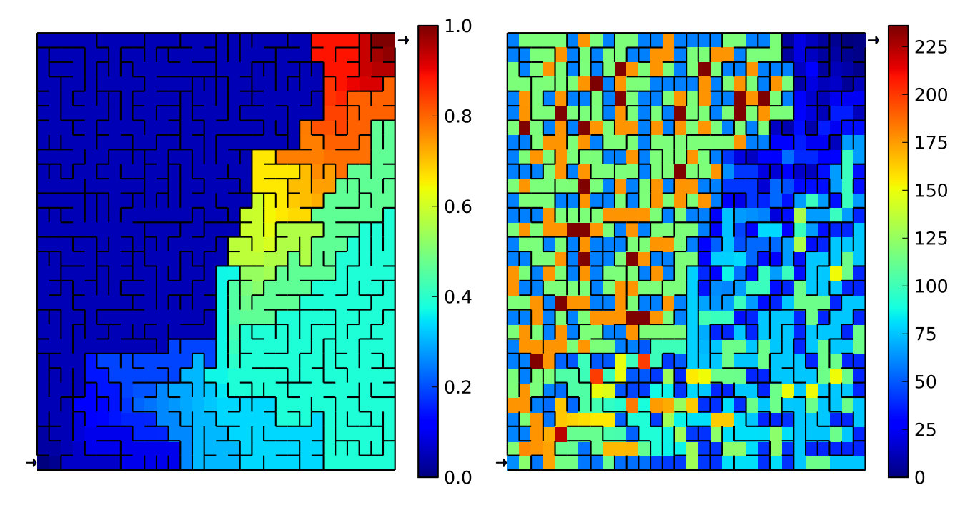 Figure 10
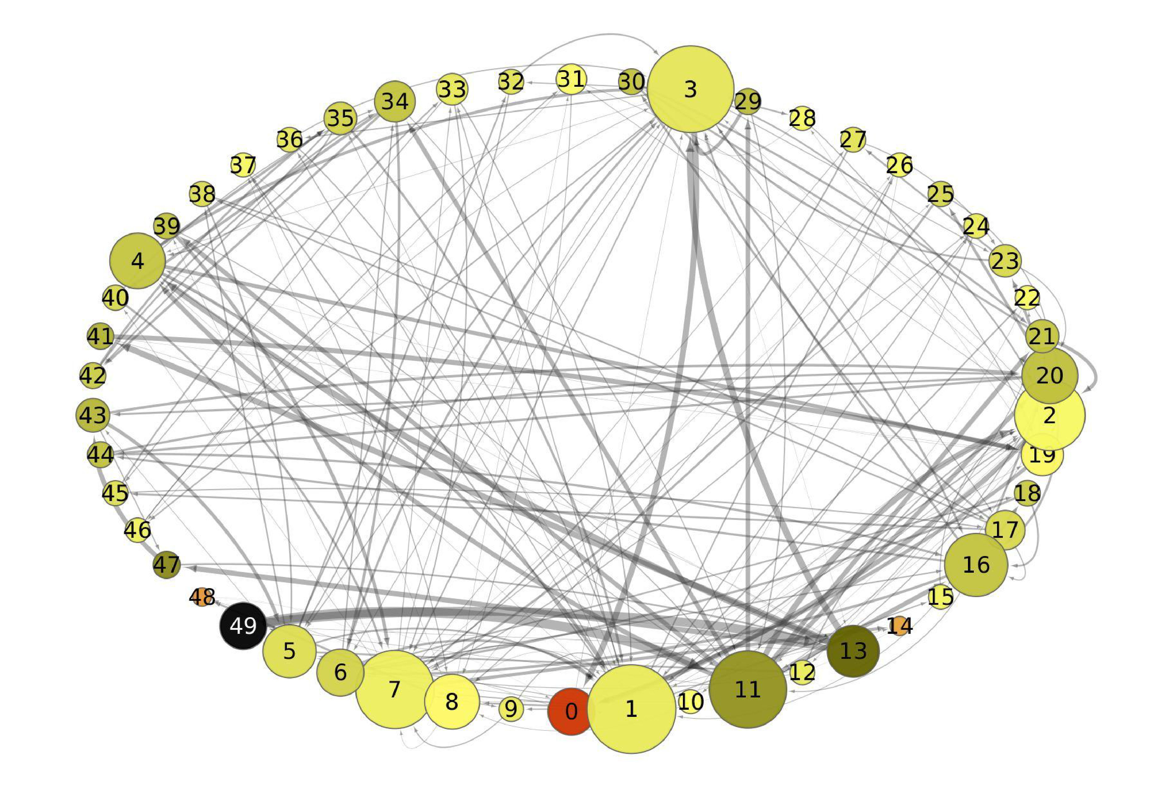 Figure 11
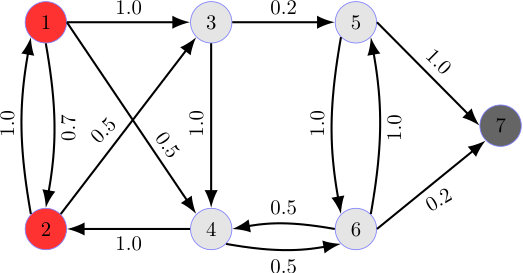 Figure 12
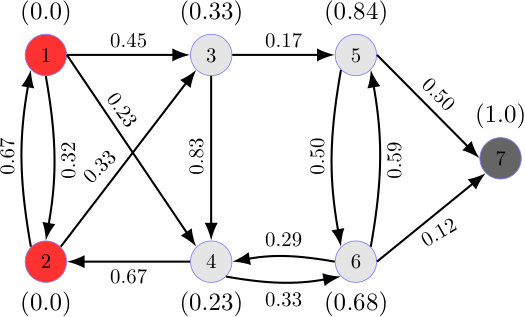 Figure 13
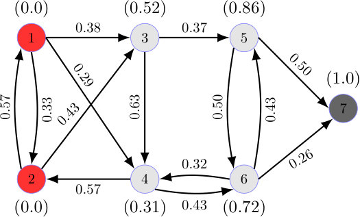 Figure 14
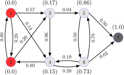 Figure 15
| set of neighbor nodes | set of sink nodes | ||
| subset of node set | subset of node set | ||
| committor function | backward committor function | ||
| invariant measure of discrete process | normalization constant | ||
| nonreactive trajectory ensemble | reactive trajectory ensemble | ||
| last hitting time of set | initial distribution on set | ||
| initial distribution of reactive trajectories | transition probability of discrete process | ||
| probability density of the waiting time along an edge | transition probability of the nonreactive trajectories | ||
| average number of times that the first passage paths visit a node | transition probability of the reactive trajectories | ||
| average number of times that nonreactive trajectories (except the last node) visit a node | average number of times that the first passage paths visit an edge | ||
| average number of times that nonreactive trajectories visit a node | average number of times that nonreactive trajectories visit an edge | ||
| average number of times that reactive trajectories visit a node | average number of times that the reactive trajectories visit an edge | ||
| probability that system stay at a node longer than certain amount of time | average total time of the first passage paths | ||
| probability density that the system jumps along an edge at a certain time | average total time of the nonreactive trajectories | ||
| average amount of time that the system stays at a node | average total time of the reactive trajectories |
| Node | Total | ||||||||
| exponential | |||||||||
| power law | |||||||||
| Weilbull | |||||||||
| Maze | |||
|---|---|---|---|
| Network | |||
| Football |
| Node | |||||||||||
|---|---|---|---|---|---|---|---|---|---|---|---|
| Degree | |||||||||||
| Node | |||||||||||
| Node | |||||||||||
| Node | |||||||||||
| Node | |||||||||||
| No. | Name | No. | Name |
|---|---|---|---|
| Neuer (GK) | Lahm (C) | ||
| Höwedes | Kroos | ||
| Hummels | Boateng | ||
| Schweinsteiger | Kramer () | ||
| Özil () | Schürrle () | ||
| Klose () | Mertesacker () | ||
| Müller | Götze () |
| Node | Node | ||||||||
|---|---|---|---|---|---|---|---|---|---|
| B | |||||||||
| B |
Peer Reviews
No public reviews on file for this paper yet. If you reviewed it on a platform where reviews are public (OpenReview, ICLR, NeurIPS, ICML), you can paste yours below so the community can read it here.
Videos
No videos yet. Explain this paper in a talk, walkthrough, or lecture? Add one.
††1 Institute of Mathematics, Freie Universität Berlin, Arnimallee 6, 14195 Berlin, Germany††2 Zuse Institute Berlin, Takustrasse 7, 14195 Berlin, Germany††Email : [email protected], [email protected], [email protected]
Statistical analysis of the first passage path ensemble of jump processes
Max von Kleist 1
Christof Schütte 1, 2
Wei Zhang 1
Abstract
The transition mechanism of jump processes between two different subsets in state space reveals important dynamical information of the processes and therefore has attracted considerable attention in the past years. In this paper, we study the first passage path ensemble of both discrete-time and continuous-time jump processes on a finite state space. The main approach is to divide each first passage path into nonreactive and reactive segments and to study them separately. The analysis can be applied to jump processes which are non-ergodic, as well as continuous-time jump processes where the waiting time distributions are non-exponential. In the particular case that the jump processes are both Markovian and ergodic, our analysis elucidates the relations between the study of the first passage paths and the study of the transition paths in transition path theory. We provide algorithms to numerically compute statistics of the first passage path ensemble. The computational complexity of these algorithms scales with the complexity of solving a linear system, for which efficient methods are available. Several examples demonstrate the wide applicability of the derived results across research areas.
keywords:
jump process, non-ergodic process, non-exponential distribution, first passage path, transition path theory
1 Introduction
(Markov) jump process has been extensively studied in the past decades and nowadays it becomes a standard mathematical model that is widely applied to problems arising from physics, chemistry, biology, etc [7, 24]. Among many important topics in the study of jump processes, the first passage paths have attracted considerable attention within different disciplines, where the main purpose is to understand the transition mechanism of the system between different subsets in state space and to e.e. access how much time the transitions typically take [21]. Examples include reaction networks in chemistry [38, 37], phenotypic switches in cell biology [39], conformational changes in molecular dynamics [17, 25], disease spreading within certain geographical areas [4, 6], as well as spread of information on social networks [16]. In these contexts, studies of the first passage paths are often very helpful to understand the underlying processes and to foster- or prevent the transition events.
A common situation that one often encounters in the study of many real-world applications is that the system exhibits metastability and transition events become very rare [27, 15, 30]. To study the transition events in these scenarios, transition path theory (TPT) has been developed both for diffusion processes on continuous state space [9, 8, 34] and for Markov jump processes on discrete state space [23, 5]. It provides a probabilistic framework to analyze the statistical properties of system’s reactive trajectories (following the terminology in [19]) and enables us to answer the questions which are important in order to understand the transition mechanism of the system. In the discrete state space setting, TPT can be applied to study Markov jump processes which are ergodic with a unique invariant measure [23, 35].
Meanwhile, inspired by the wide applications that have emerged due to the rapid development of network science, scientific interest has been extended to study processes which go beyond ergodic Markov jump processes [26, 29, 28]. One simple example when ergodicity is violated is the random walk on a directed graph which contains sink-states (states with no outward edges). Another example of a non-Markovian process is the continuous-time random walk with possibly non-exponential waiting time distributions. These kind of processes have been applied to model the burst and memory effects in real-world networks [13, 20, 10]. The above described processes are no longer ergodic Markov jump processes and therefore TPT can not be applied directly. However, interesting insights can be obtained when studying the transition mechanism from one subset to another, to determine how much time the transitions typically take and to identify key nodes or edges for the transition events. To our best knowledge, these questions have not been systematically addressed in the non-Markovian and non-ergodic setting (see related study in [20]).
In the current work we consider the first passage path ensemble of both continuous-time and discrete-time jump processes on a discrete, finite state space. While we are strongly influenced by TPT and will study similar quantities such as the probability of visiting each node and probability fluxes on each edge, we emphasize that both the subject being studied and the setting are different from the study of TPT [23, 5]. Specifically, we will study the first passage path by dividing it into nonreactive and reactive segments. While in the ergodic case the reactive segments coincide with the reactive trajectories in TPT, in this work we also study the statistics of nonreactive segments and their relations with the statistics of the entire first passage paths. Furthermore, in our study the processes are allowed to be non-ergodic, and in the continuous-time scenario the waiting time on each node can be also non-exponentially distributed. The main contributions of this paper can be summarized as follows. Firstly, statistical properties of both nonreactive and reactive path ensembles have been analyzed, which enables us to compute several important quantities associated to the reactive- and nonreactive ensembles. Their relations to the entire first passage path ensemble are obtained subsequently. Secondly, since the processes are not necessarily ergodic or in stationary anymore, our analysis (of the reactive segments) can be viewed as an extension of TPT to nonequilibrium path ensembles. When further assuming that the processes are ergodic Markov jump processes and the first passage path ensemble is in equilibrium, our analysis recovers TPT and allows to elucidate the statistical connection between transition paths in TPT and the first passage paths. Thirdly, the numerical implementation of the derived results is discussed, which is useful in many applications.
The paper is organized as follows: The first passage path ensemble of discrete-time Markov jump processes is studied in Section 2. The first passage path ensemble of continuous-time jump processes with general waiting time distributions is considered in Section 3. Connections of our analysis with TPT are discussed in Section 4 where we recover the results of TPT when the processes are ergodic and the path ensemble is in equilibrium. Algorithmic issues are discussed in Section 5 and several numerical examples are presented in Section 6 to illustrate our analysis framework. Conclusions and further discussions are present in Section 7. Finally, some supplementary analysis related to Section 2 and Section 3 is provided in Appendix A and Appendix B.
For the reader’s convenience, important notations which will be used in the current work are summarized in Table 1.
2 Analysis of the first passage path ensemble : discrete-time Markov jump processes
In this section, we study the first passage path ensemble when the system is a discrete-time Markov jump process. After introducing various useful notations in Subsection 2.1, we will analyze the statistics of the nonreactive ensemble and the reactive ensemble in Subsection 2.2 and Subsection 2.3, respectively. Their connections with the whole first passage path ensemble are discussed in Subsection 2.4.
We also emphasize that although several quantities that we will consider are strongly influenced by TPT, the main difference is that they are related to the first passage path ensemble which may be out of equilibrium and therefore do not reply on the existence of invariant measure. Connections of our analysis with TPT will be further discussed in Section 4.
2.1 Preparations
We start by introducing the processes we will consider and the notations that will be used in this paper. Let be the graph representation of a directed network , where is the set of nodes and is the set of edges. We assume that is a finite set and, without loss of generality, for some . We will write if and denote as the set consisting of all nodes which can be directly reached from node . For simplicity, we assume that there are no loop edges in , i.e. , for . Since we are also interested in the case when the network contains sinks, we allow the case when for some node and denote to be the set of sink nodes.
Suppose that two disjoint nonempty subsets are given. And let be a probability distribution on set . Consider the discrete-time Markov process defined by the jump probability for , which is the probability that the system will jump to state if its current state is . Given node , we define two stopping times related to sets
[TABLE]
and set (or ) if the process will never reach set (or ) from . Especially, we have for and for . Assume the process starts from some node and consider the path until it reaches set . Denote the path as , then we have , , where and for . Such a path is called the first passage path [6, 21]. We also define the last hitting time of set as
[TABLE]
and set , if for . In the following, we will use the notations , and for simplicity if we do not explicitly emphasize the initial state .
Given any first passage path starting from a state in set (therefore ), we can split this path into two segments using the last hitting time . The first segment , which will be termed as nonreactive trajectory or nonreactive segment, consists of the consecutive nodes visited by the process before it eventually leaves set . The second segment , which is called reactive trajectory in transition path theory [23], is the transition pathway of the process from set to set (see Figure 1(a) for illustration). We will call it either reactive trajectory or reactive segment. Equivalently, the reactive trajectory is the segment of the first passage path starting from some node in which is hit by the process for the last time. Clearly, we have and for . The ensembles of the nonreactive trajectories and reactive trajectories are denoted by
[TABLE]
respectively, where goes over all first passage paths with initial state and .
Given a node , we say that set (or ) is reachable from , if there is a path of finite length , where , such that , (or ), , , and , . Throughout the paper, we will make the following assumption.
Assumption 1**.**
. For each node , either set or set is reachable from . Furthermore, set is reachable from each node .
Under the above assumption, we can conclude by contradiction that with probability for all . Therefore, the committor function,
[TABLE]
corresponding to sets is well defined and will play an important role in the following study. It is known that it satisfies the equations [23]
[TABLE]
We also define two subsets
[TABLE]
Clearly, we have and , where the latter is implied by Assumption 1 together with the following result.
Proposition 1**.**
Let be the last hitting time defined in (2) and subsets be defined in (6). We have
, . 2. 2.
* iff and set is reachable from node .* 3. 3.
* iff and set is reachable from node .*
Proof.
We will only prove the first two conclusions since the third one can be obtained using a similar argument as the second one.
By definition of , we know that the two events and are equivalent. It follows from the definition of in (4) that . 2. 2.
Suppose . Using the definition of , we know with a positive probability, which implies that set is reachable from . Conversely, suppose and set is reachable along the path . If , then and . Applying equation (5), we obtain . As for , we can repeat the argument and obtain . However, this contradicts the fact that since . Therefore we have .
∎
From Proposition 1, we know that Assumption 1 implies and .
2.2 Nonreactive ensemble
In this subsection, we study the nonreactive ensemble defined in (3). Given a nonreactive trajectory , where and is the last hitting time defined in (2), it is clear that for (Proposition 1). Our aim is to define a Markov jump process whose path ensemble coincides with . For this purpose, we first introduce a virtual node [math] to mark the end of the path and consider the extended node set . A jump from some node to node [math] indicates that is the last node of the nonreactive trajectory. We also define the transition probability from node to as
[TABLE]
and . Using (5), we can verify that is a probability matrix on set with row sum one. Furthermore, we have
Proposition 2**.**
The ensemble can be generated by trajectories (without the end node [math]) of the Markov jump process on space with transition probability matrix in (10) and initial distribution .
Proof.
Let be one nonreactive trajectory such that . For and , using the Markov property and the definition of the committor function , we can compute
[TABLE]
For , event is equivalent to the event that the original process (on ) hits set first (before it returns to ) after it leaves set from node . The probability of the latter is equal to and therefore coincides with the probability that the process (on ) jumps from to [math]. The case for can be argued using a similar argument. ∎
Given , let be the average number of times that node is visited by the nonreactive trajectories, i.e.
[TABLE]
where is the indicator function, denotes the ensemble average of , or equivalently, the ensemble average of the first passage paths with the initial distribution . It is straightforward to verify
[TABLE]
Furthermore, we have
Proposition 3**.**
For , function defined in (11) satisfies the equation
[TABLE]
where probabilities are given in (10).
Proof.
Using Proposition 2, we can rewrite the transition probabilities using the ensemble average, i.e.
[TABLE]
where and we have set , which marks the end of the nonreactive trajectory. Therefore, using the definition of in (11) and summing up , we obtain
[TABLE]
Since , we know and therefore
[TABLE]
where we have used the definition of again and the fact that . ∎
Especially, summing up in (13) and using the fact that has row sum one, we can verify the equality
[TABLE]
It is also useful to introduce
[TABLE]
which is the probability distribution of the last hitting node on set and satisfies (see Figure 1 (b) for illustration). Furthermore, in analogy to (11), we define
[TABLE]
which coincides with on and the summation above is interpreted to be zero when . The following relations are straightforward.
Proposition 4**.**
Let and the probabilities be defined in (11) and (10), respectively. Then for ,
[TABLE]
Proof.
We only need to prove the first equality in (19). Notice that (17) can be written as
[TABLE]
where we have used the convention that . Similarly as in (14), applying Proposition 2, we have
[TABLE]
Therefore, we conclude that
[TABLE]
∎
We also introduce the nonreactive probability flux, which is defined as
[TABLE]
and equals zero for other edges in . From (11) and (14), can be written as a path ensemble average
[TABLE]
i.e. the average number of times that edge is visited by the nonreactive trajectories. Applying Proposition 3 and Proposition 4, we have
Corollary 1**.**
[TABLE]
2.3 Reactive ensemble
In this subsection, we turn to study the reactive ensemble in (3). First of all, from the definition (3), we know that the probability distribution of the initial state of the ensemble coincides with the probability distribution of the end node in the ensemble . See (17) and Proposition 4 (an alternative derivation can be found in Appendix A).
Now recall the definition of set in (6), Proposition 1, and also notice that . In analogy to the previous subsection, our aim is to construct a Markov jump process on space whose path ensemble coincides with . To do so, we define the transition probabilities
[TABLE]
where , and is the delta function centered at . We have the following result (the proof is omitted since it is similar to Proposition 2; Note that a similar result under the assumption of ergodicity has been obtained in [5]).
Proposition 5**.**
The ensemble can be generated from the trajectories of the Markov jump process on space which is defined by the transition probabilities in (26) and the initial distribution on .
For , let be the average number of times that node has been visited by reactive trajectories, i.e.
[TABLE]
where is a first passage path and denotes the corresponding ensemble average. Clearly when . Summing up in (27), we can obtain
[TABLE]
Similar to Proposition 3, we have
Proposition 6**.**
Let be the transition probability defined in (26). We have for , and
[TABLE]
Especially, .
Proof.
Since nodes of set appear in reactive trajectories only as the starting state with probability distribution , we have on . Equation (29) can be proved in an analogous way to Proposition 3, by rewriting as the ensemble average and applying Proposition 5. See (14). By the definition of the stopping time , we know for . Therefore, from (27),
[TABLE]
Summing up and using the fact that , we conclude
[TABLE]
∎
Remark 1**.**
Notice that (29) holds for node as well. For numerical computation, we can first compute for by solving the linear system (29), and then obtain the end node distribution for each from (29).
For each edge , , , we define the reactive probability flux as
[TABLE]
and set it to zero for other edges in . In analogy to (21), we have the ensemble average representation
[TABLE]
where is a first passage path and denotes the corresponding ensemble average. Applying Proposition 6, we can obtain
Corollary 2**.**
Let be the reactive probability flux defined in (30) and be given in (27). We have
[TABLE]
Proof.
It follows directly by applying (30), Proposition 6, and the fact that row sums of matrix are one. ∎
2.4 First passage path ensemble
Based on the previous analysis of the nonreactive and reactive trajectories, we study the whole first passage path ensemble in this subsection.
Given , we define as the mean first hitting time of set for the discrete-time Markov jump process starting from , i.e. . Using Markovianity, we can write it as
[TABLE]
It is also well known that satisfies the equations
[TABLE]
Accordingly, if the probability distribution of the initial state on set is , the average length of the first passage path is then given by . Also, let be the average number of times that node has been visited by the first passage path with initial distribution , i.e.
[TABLE]
In analogy to Proposition 3 and Proposition 6, we know it satisfies
[TABLE]
Furthermore, taking into account the definitions of , and in (11), (18) and (27), as well as relations (12), (28), we can verify the following relations
[TABLE]
In fact, the following explicit relations hold.
Proposition 7**.**
For any ,
[TABLE]
Proof.
Clearly if . Hence we only need to consider the case when . Using the Markov property, we can compute the probability from the first passage ensemble. Specifically, let be a first passage path. Conditioning on where , the event is actually equivalent to . Therefore,
[TABLE]
which implies \bar{\theta}(x)=\theta(x)\big{(}1-q(x)\big{)}. The expression of follows from (37). ∎
We also introduce the probability flux for edge , which is defined as
[TABLE]
[TABLE]
And the following result is straightforward.
Proposition 8**.**
For , we have , or equivalently,
[TABLE]
Proof.
(41) follows directly from the ensemble average representations of fluxes in (40), (21), (31). ∎
3 Analysis of the first passage path ensemble : continuous-time jump processes
In this section, we turn to study the first passage path ensemble of continuous-time jump processes with general waiting time distributions. After introducing the process and some notations, we will derive a discrete-time Markov jump process which encodes the dynamical information of the original continuous-time process. Applying the analysis in Section 2 to this discrete-time Markov jump process, we are able to analyze the first passage path ensemble of the continuous-time jump process.
3.1 Preparations
We consider a continuous-time jump process on network . We will follow the derivations in [13] and some extra notations are needed in order to introduce the process. A related study on the continuous-time jump processes can also be found in [20].
Following Subsection 2.1, let us first assume that node and consequently . From node , the system may jump to one of the nodes in after staying at for a certain duration of time. We assume that the jump events at each node are independent of each other, and denote the probability density of the waiting time as , conditioning on that the system jumps from to another node . As a probability density function, it satisfies . Let be the probability that the system stays at node for a time longer than before it leaves. Also denote the probability density that the system jumps from node to at time by . Since we have assumed that the jump events to different nodes are independent of each other, it is straightforward to verify that
[TABLE]
and they satisfy the equation
[TABLE]
We also know that the average time the system will stay at a node is
[TABLE]
Let be the probability that the system jumps from node to , regardless of when the jump event occurs, then we have
[TABLE]
and , for . From (42) it follows and, taking the limit in (43), we can obtain
[TABLE]
We also assume that the process will terminate once it reaches one of the sink nodes. Correspondingly, for , we set , , and therefore the equality is still satisfied. In other words, is a probability matrix and therefore defines a discrete-time Markov jump process on . As further presented in Appendix B, this discrete-time Markov jump process encodes the dynamical information of the original continuous-time process. And it will be useful in the following Subsection 3.2.
For general probability densities , numerical integrations are needed in order to compute transition probabilities from (42) and (45). In the following, we discuss three special cases [10, 32] when the analytical expressions of can be obtained (see Figure 2).
Exponential distributions. The probability densities are
[TABLE]
for some , where . It corresponds to the continuous-time Markov jump process and we can define the generator matrix of the process whose entries are
[TABLE]
for , and , , when . From (42), (45) we can obtain that, for ,
[TABLE] 2. 2.
Weibull distributions. In this case, we assume
[TABLE]
for some and , where . From (42), (45) we can obtain that, for ,
[TABLE]
where is the Gamma function. Clearly, we recover the exponential distribution when . 3. 3.
Power law distributions. In this case, we assume
[TABLE]
for some , where . From (42), (45) we can obtain that, for ,
[TABLE]
3.2 Path ensemble analysis
In this subsection, we study the path ensemble of the continuous-time jump process by applying the analysis in Section 2 to the discrete-time Markov jump process obtained in the previous Subsection 3.1. The structure of the contents is the same as in Section 2 and therefore only the necessary steps in order to adapt the analysis to the continuous setting will be summarized.
Nonreactive ensemble
For the nonreactive ensemble, denoting as the continuous-time jump process introduced in Subsection 3.1 and following Subsection 2.2, we define
[TABLE]
to be the average amount of time that the nonreactive trajectories spend at node . Notice that we denote as the time when the th jump occurs and especially is the last hitting time of set . Recall (44), we have
[TABLE]
and therefore the average total amount of time of the nonreactive trajectories is
[TABLE]
Reactive ensemble
For the reactive ensemble, similar to (57), we define
[TABLE]
which is the average amount of time that the reactive trajectories spend at node . From (44), we have
[TABLE]
and therefore the average total amount of time of the reactive trajectories is
[TABLE]
First passage path ensemble
For the first passage path ensemble, following Subsection 2.4, we define
[TABLE]
which is the average amount of time that the first passage trajectories spend at node . Similarly as above, we can obtain
[TABLE]
where are defined in (57), (60), and the average total amount of time of the first passage trajectories is
[TABLE]
4 Ergodic case : connections with TPT
In this section, we consider the special case when either the original process or, in the continuous-time case, the discrete-time Markov jump process obtained in Section 3 is both irreducible and aperiodic. In this case, statistics of the transition (reactive) segments have been studied in TPT by embedding these segments into an infinitely long stationary trajectory. Our key observation is that in fact they can be embedded into the first passage path ensemble with certain initial distribution and therefore can be studied by applying the analysis in the previous sections. This approach elucidates the relations between the study of the first passage paths and the study of the transition paths in TPT.
To proceed, we first notice that in this case Assumption 1 in Section 2 is satisfied and indeed we have in (6), . The discrete-time jump process is ergodic and we assume its unique invariant measure is such that [24, 18]. We also introduce the time reversed process defined by the transition probabilities , and the backward committor function which satisfies the equation
[TABLE]
It is known that equals to the probability that, being at , the process came from set rather than from set [23, 34].
We can further assume that there is an infinitely long trajectory of the discrete-time jump process, where , . To make a connection with the general case studied in the previous subsections, we introduce the stopping times , and
[TABLE]
where . Similarly as in (2) and (3), we define
[TABLE]
and consider the ensembles of the equilibrium nonreactive and reactive segments
[TABLE]
constructed from the infinitely long trajectory . Using the definition of , we can obtain the expressions of the various quantities related to ensembles (69) in the ergodic setting.
Proposition 9**.**
Consider the path ensembles and in (69).
For the normalization constant, we have
[TABLE] 2. 2.
The initial distribution (on set ) of the ensemble satisfies
[TABLE] 3. 3.
Let be defined in (35), we have
[TABLE] 4. 4.
Let be the initial distribution of , and , be defined in (11), (27) respectively. We have
[TABLE]
Proof.
We have
[TABLE]
And it follows from (66) that
[TABLE]
Therefore, using , , from (77) we obtain
[TABLE]
which implies (70). 2. 2.
Using Markovianity of the discrete-time jump process and the definition of , we can derive
[TABLE]
where means “equal up to a constant” and the normalization constant is given in (70). 3. 3.
Using the equation of in (66) and the formula of in (71), it is easy to verify that defined in (75) satisfies equations (36). 4. 4.
The expressions of , and follows from (75), Proposition 4 and Proposition 7.
∎
Remark 2**.**
Using the expression of in (76) and an argument similar to the proof of (70), we could obtain
[TABLE]
Finally, we consider the continuous-time jump process introduced in Section 3 and assume its associated discrete-time Markov jump process obtained in Subsection 3.1 is ergodic. In this case, we consider an infinitely long trajectory of the process as in (93) in Appendix B and let be the integer such that , where the stopping times are defined in (67). Following [23], we define the reaction rate between sets and by
[TABLE]
We have the following result.
Proposition 10**.**
Consider the continuous-time jump process introduced in Subsection 3.1. Let be defined in (44). are the transition probabilities and the committor function of the associated discrete-time Markov jump process defined in (45), (4), respectively. Suppose that this discrete-time jump process is ergodic with a unique invariant measure . We have
[TABLE]
Proof.
We consider the path in (93) in Appendix B which jumps from state to at time , . We also denote its state at time as . Using the Markov property and ergodicity of the discrete-time jump process, we have
[TABLE]
On the other hand, we have
[TABLE]
Therefore,
[TABLE]
Combining (81) and (82), we can conclude that
[TABLE]
∎
Remark 3**.**
We conclude this section with the following remarks.
From (78) in Remark 2, we know the numerator in the expression (80) equals the constant and can be replaced by the other expressions in (78). 2. 2.
The case when the continuous-time jump process itself is Markovian and ergodic has been studied in **[23]**. The invariant measure in **[23]** of the continuous-time process is related to and in the present work by
[TABLE]
Together with formulas in (52), we can verify that Proposition 9 and Proposition 10 are accordant with the results in **[23]**. Therefore, we have extended the analysis there to more general continuous-time jump processes introduced in Subsection 3.1.
5 Algorithmic issues
In this section, we briefly discuss some algorithmic issues related to applying the analysis of Section 2 and Sections 3 to applications.
5.1 Summary of the analysis procedure
Given a continuous-time or discrete-time jump process on a finite state space, the analysis of its first passage paths can be proceeded as follows.
Construction of the discrete-time network.
The analysis of the current work can be applied to both continuous-time and discrete-time jump processes. In the case of a continuous-time jump process, we have shown in Section 3 how the transition probabilities of the corresponding discrete-time Markov jump process (without time information) are related to the probability density function of the waiting times. For certain probability density , analytical formulas of , as well as other quantities in Section 3 can be obtained. For more general probability densities, however, numerical integration is needed in order to compute , using formulas (42), (45) and (44). 2. 2.
Calculation of the statistics of path ensembles. After obtaining transition probabilities , we can compute various statistical quantities of the nonreactive ensemble, reactive ensemble, as well as the entire first passage path ensemble. While the equations for each quantity have been derived in Section 2 and some quantities can be obtained in several ways, we suggest to proceed in the order which is summarized in Algorithm 1. In the ergodic case where the initial distribution is given in (71), we could either first obtain from the backward committor equation (66) and compute the other quantities using Proposition 9, or follow the procedure in [23].
Among the steps in Algorithm 1, the only possible computational difficulties are related to solving the linear systems (5) and (36). Using numerical packages such as PETSc [3], however, these linear systems can be easily solved for (sparse) networks with several thousand nodes and therefore the algorithm could be used in a wide range of applications.
Post-processing. The various statistics obtained above allow us to better understand the mechanism of the system’s transitions from one set to another. However, how to interpret and represent these information is a nontrivial question and indeed depends on the problem at hand. In some cases, the key interest is to find certain important pathways which the system is likely to take [9, 34, 23]. Algorithms for computing dominant pathways in the network setting have been studied in [23, 17, 36]. In general, however, the first passage paths of the system may be typically very long and diffusive. In this case, presenting the statistics by identifying a single representative pathway may be incomplete or even misleading (see examples in Section 6). In the current work, instead of discussing in detail specific methods to further exploit the statistics, we simply point out that one can rank the importance of nodes and edges based on these statistics. Specifically, taking the reactive trajectories as an example,
- (a)
By ranking nodes according to committor function , we can figure out how “close” each node is to the initial set and to the terminal set . (Here the closeness is measured by the committor probability). 2. (b)
By ranking nodes according to function , we know which nodes are more frequently visited by the reactive trajectories. 3. (c)
By ranking edges according to flux , we know which edges are more frequently visited by the reactive trajectories.
In the case of the continuous-time process, ranking can be also based on so that we could identify nodes on which the process will spend more time. Certainly, similar rankings allow us to identify nodes and edges which are important for the nonreactive trajectories, as well as for the entire first passage paths.
5.2 Data-based approach
In various real-world applications, we may face the situation that the system’s information is not available, i.e. or are unknown, and only the trajectories of the system can be observed. In this case, one usually takes a data-based approach and constructs a Markov jump process from the available data. Specifically, suppose that we have obtained trajectories of the system. For the th trajectory, , it starts from at time and jumps to state at time , , before it reaches set at time for the first time. That is, for and . Also define to be the last time when the th trajectory visits set . It satisfies , and for . Then a natural way to estimate the function and transition probabilities is given by
[TABLE]
where , provided that the denominator is nonzero. Similarly, for the initial distribution , we can estimate
[TABLE]
where . Detailed studies related to the reconstruction of the Markov jump processes from data can be found in [22, 27] and references therein.
After estimating and from (84), we can follow Algorithm 1 and the discussions in Subsection 5.1 to perform the analysis. In fact, direct calculation shows that function and flux in (35) and (40) are simply given by
[TABLE]
In other words, instead of solving the linear system (36), the ensemble average and of the constructed Markov jump process can be obtained by “counting” the trajectory data. However, we emphasize that this is not true in general for other quantities of ensemble averages. For instance, generally, the committor function and quantity , which satisfy equations (5) and (13) respectively, are different from
[TABLE]
which are computed by “counting” the trajectory data. As a simple counterexample, consider graph with four nodes . We define sets and suppose that only trajectories , are observed (time information is ignored for simplicity). Then clearly , , and it follows from (87) that , . On the other hand, from (84), we have , and it follows that as a consequence of Proposition 1. Similarly, we can also show that .
In summary, after obtaining transition probabilities from (84), one still needs to apply Algorithm 1 to obtain various statistical quantities. In the first step of Algorithm 1, although function can be calculated from (86), it is necessary to compute the committor function by solving the linear system (5).
6 Numerical examples
In this section, we study several examples in order to demonstrate the analysis in the previous sections.
6.1 Example : continuous-time jump processes on a simple graph
As the first example, we consider continuous-time jump processes on a graph which consists of nodes. As shown in Figure 3 (a), we choose sets , , and study jump processes starting from set until they reach set . We assume the initial distribution is uniform on , i.e. . Three different cases are considered, i.e. when the waiting time at each node satisfies (i) an exponential distribution, (ii) a power law distribution and (iii) a Weibull distribution, respectively (see Subsection 3.1).
In both cases of the exponential and Weibull distribution, we take the same rate constants in (47) and (53), which are shown in Figure 3 (a) for each edge , where is used for each edge in the Weibull distribution. In the case of the power law distribution, we choose in (55) to be equal to for each edge , such that the mean of the waiting time along each edge is the same as in the case of the exponential distribution.
In each case, starting from the continuous-time jump processes, we first construct the corresponding discrete-time jump processes using relations (42), (45) in Section 3. The transition probabilities for each edge as well as the committor function for each node are shown in Figure 3 (b)-(d). Clearly, different assumptions on the waiting time distributions of the continuous-time jump processes result in discrete-time Markov jump processes with different transition probabilities. In fact, from the formulas of transitions probabilities in (52), (54), we can conclude that, comparing to the exponential distribution case, the difference between jump probabilities along edge and edge where will be larger when the waiting times follow Weibull distribution with . Furthermore, it can be observed that comparing to the exponential distributions, the probabilities to jump from “left to right” (e.g. along edges , and ) are larger in the case of power law distributions, and are smaller in the case of Weibull distributions ().
The ensembles of the nonreactive segments, the reactive segments, as well as the whole first passage paths are studied following the analysis in Section 2 and Section 3. The ensemble averages , , , , and for each node in different cases are shown in Table 2. Also see Figure 4 where these quantities are displayed in the case of the exponential distribution. We refer to equations (18), (27), (35), (57), (60), (63) as well as Table 1 for definitions of these quantities. In each case, from the values of the quantity we can observe that the system will typically visit nodes and return to set a few times before it eventually arrives at set . As shown in the columns with label “Total” in Table 2, we also see that while in each case the reactive trajectories contain a similar number of jumps on average (–, last column rows , , ), there are fewer jumps within the nonreactive trajectories in the case of power law distribution (), but on the other hand there are more jumps in the nonreactive trajectories in the case of the Weibull distribution (). The same is also true for the first passage paths as well as when we take time information into account. These results are accordant with our previous observations based on Figure 3 (b)-(d) that transitions of the system from set to are more difficult when the jump time follows the Weibull distribution.
6.2 Example : discrete-time random walk in a maze
In this subsection, we consider a (discrete-time) random walk in a maze. This example has been considered to illustrate TPT in [9]. However, since the theory there requires ergodicity of the process, an implicit assumption one need to make is that the walker keeps moving in the maze even after arriving at the exit cell. In this work, we investigate the same example (except we don’t have to make the aforementioned assumption) and apply the analysis in Section 2 to study its path ensembles.
The maze is constructed on a grid and the structure is shown in Figure 5. We assume that the walker enters the maze from the cell at the bottom left corner. At each unit of time, the walker moves to a new cell which is chosen randomly with equal probability from all neighboring cells that are directly reachable from the current one (no wall in between). The walker keeps moving until it finally arrives at the upper right corner where it can leave the maze.
To apply the analysis in Section 2, we construct an undirected graph whose nodes consist of the cells of the maze and two nodes are connected by an edge if and only if the corresponding cells in the maze are adjacent and there is no wall in between. Sets , consist of a single node corresponding to the cell at the bottom left and the upper right corner (see Figure 5), respectively. Since the process itself is a discrete-time Markov jump process, its transition probabilities can be directly computed from the connectivity structure of the maze. Committor function and function related to the first passage paths are shown in Figure 6. From the committor function , we can observe that there are long vertical walls which roughly separate the maze into left and right parts. In the left part (dark blue cells in the left panel of Figure 6), the walker is likely to return to first before it goes to . On the other hand, from the plot of the function in the right panel of Figure 6, we can realize that, unlike the simple pathway shown in Figure 5, the first passage paths from to taken by the walker are very diffusive on average, since many cells have been repeatedly visited within a single first passage path. The diffusiveness of the paths can also be observed from the very long average path lengths in Table 3.
In order to further investigate the nonreactive and reactive segments of the first passage paths, functions , are computed and are shown in Figure 7. We can see that both of these two segments are diffusive on average, since many cells are repeatedly visited. Comparing these two segments, however, it is observed that a large number of the visits at cells in the left part of the maze actually belong to the nonreactive segments and do not contribute to the reactive pathways. Comparing the two panels in Figure 7, we can also conclude that the nonreactive segments are typically more diffusive than the reactive segments. Roughly speaking, this phenomena occurs similarly when studying the transitions of a metastable diffusion process between two local minima of a potential, where the system spends longer time in the basin of attraction than in the transition region.
6.3 Example : discrete-time random walk on a scale-free network
In this example, we consider a network with a power law degree distribution. The network is generated using Python package NetworkX [11], which implemented the algorithm of Holme and Kim [14] to generate growing graphs with power law degree distribution. In order to have a better illustration, we choose a relatively small network with nodes. During the growth of the network, two random edges are added for each new node and the probability of adding a triangle after adding a random edge is [11]. The structure of the network is shown in Figure 8.
To continue, we take the discrete-time random walk on this network as an example and study its first passage paths starting from node to node [math], i.e. . Various statistics are computed following Algorithm 1, as well as the methods presented in Section 5. In Table 4, nodes are ranked according to different statistics and part of them are listed. It can be observed that, except for the source node , the committor values of all other nodes are larger than , reflecting the fact that these nodes are more tightly connected to node [math] compared to node , which is the last node added during the growth of the network. We can also conclude that nodes with large values tend to have large values of (or ) and as well. Furthermore, a positive correlation can be observed between the magnitudes of these statistics and the degrees of nodes, which probably could be explained by the undirected (symmetrical) movement of the random walker. In Figure 8, information related to the reactive trajectories are shown. Specifically, nodes with larger values are indicated by brighter colors, and nodes with larger values are displayed in larger sizes. Also, edges with larger reactive fluxes are plotted using thicker lines. From Figure 8, we could identify nodes and edges that are more frequently visited by reactive trajectories. The average path lengths of the nonreactive trajectories, the reactive trajectories, as well as the whole first passage paths are shown in Table 3. Different from the previous maze example, the lengths of the reactive trajectories are longer than those of the nonreactive trajectories on average, which is due to the fact that the attraction of the source set is not strong.
Summarizing the above results, we can conclude that, due to the global connectivity of the network, the path ensembles are widespread in path space and it is difficult to identify certain dominant transition pathways for this system. But still, we have obtained insights about the transitions of the random walk both quantitatively and graphically.
6.4 Example : football match
In the last example, we apply the analysis in Section 2 to study the football match between Germany and Argentina in the world cup final [1]. The main aim is to quantify the performance of the players according to the ball passes during the match. For simplicity, we only focus on the German national team and model the ball passes between players as a discrete-time Markov jump process.
We take the data-based approach as discussed in Section 5. First, all passes between players of the Germany national team during the entire game ( minutes plus minutes extra time) were recorded [2]. These passes constitute trajectories, each of which describes consecutive ball passes among German players when the team possessed the ball. Since each trajectory may start or finish in different ways, besides the starters and substitutes who participated in the game (see Table 5), additional nodes are introduced in the state set as outlined below. Specifically, a trajectory starts from node if the goalkeeper starts with a kick, and it starts from either node S[math] or node S when the Germany team got the possession from the opponent (or via a throw-in), depending on whether it occurred in the defensive Half or attacking Half. Similarly, for the end state, node L[math] and L indicate that the German team lost possession of the ball in the defensive Half and attacking Half, respectively. Furthermore, both nodes B[math] and B mark that the attack finished in the opponent’s penalty area, while the latter indicates a shot on goal was made.
We estimate the transition probabilities and the initial distribution of the graph using formulas (84), (85) in Section 5. Besides the three initial nodes S[math], S and (Neuer), we also select nodes , and into the set , since they correspond to the three full-back players (Höwedes, Hummels, Boateng) who stayed in the defensive Half most of the time during the match. Therefore, we have sets and the initial distribution for nodes S[math], S, , , , 20$$\} in set is . Set is chosen to contain all end nodes of the trajectories, i.e. . This choice of set allows us to utilize all the trajectories and the results can provide us an overall insights of this specific match, i.e. not only shots on goal but also attacks which were not successful.
After these preparations, we apply Algorithm 1 to compute the various statistics defined in Section 2 and results are shown in Figure 9 and Figure 10. As already mentioned in Section 5, function , flux and the average total length of the first passage paths computed from Algorithm 1 are identical to those computed from estimators in (86). In Figure 9, nodes and edges are displayed in different sizes and thickness according to the values of function and flux . It could be observed that the four players Schweinsteiger, Kroos, Lahm, Özil had much possession of the ball and contributed more ball passes compared to the other players. In Figure 10, on the other hand, the sizes of nodes and the thickness of edges are determined according to their values of function and , respectively, which are related to the reactive trajectory ensemble. We see that passes among the goalkeeper and the full-back players (Neuer, Höwedes, Hummels, Boateng) are filtered out. Furthermore, upon closer examination of the edges, we can observe that the role of the attackers (e.g. Özil, Müller) become more prominent. Quantitative results are presented in Table 6.
7 Conclusions
In the present work, we have developed a theory for the statistics of the first passage path ensemble of jump processes on a finite state space. The main approach is to divide a first passage path into nonreactive and reactive segments so that the behaviors of the processes within each segment can be studied separately. Furthermore, relations between the statistics of these two segments and the statistics of the entire first passage paths are obtained.
Our analysis can be applied to jump processes which are non-ergodic, as well as continuous-time jump processes where the waiting time distributions are non-exponential. More generally, second-order or higher order Markov chains have been studied where the dynamics depend not only on system’s current state but also on the states which have been visited in the previous steps [28, 29, 31]. These types of jump processes can be converted to Markov jump processes by extending the state space and therefore it is possible to apply the analysis in the current work to study these higher order Markov chains (although the size of the extended state space may become quite large and brings computational difficulties).
We expect that the study of both the nonreactive and reactive segments can help to understand the transition behavior of processes from one subset to another. Especially, analysis of the reactive segments in this work is closely related to TPT, which was developed for both diffusion processes and jump processes under the assumption of ergodicity. Some illustrative examples are studied numerically in order to demonstrate the applicability of the theory. More generally, the study of the transition events, or the first passage phenomena [21], plays an important role in order to understand many real-world systems and applications, e.g. in molecular dynamics or in epidemiology. Applying the analysis of the current paper to study phenomena in the aforementioned subject areas will be considered in future work.
Acknowledgement
This research has been funded by Deutsche Forschungsgemeinschaft (DFG) through grant CRC 1114, by the Einstein Foundation Berlin through project CH4 of Einstein Center for Mathematics (ECMath) and though the BMBF, grant number 031A307.
Appendix A An alternative expression of
Here we provide an alternative way of studying the probability distribution defined in (17) in Section 2. Consider the first passage paths starting from , and for each , let be the probability that is the last hitting node in , i.e. . The equation of can be obtained by considering the next state which the system will jump to from . In the case , we obtain the relation
[TABLE]
Notice that for , we have and (88) still holds.
In the case , after jumping to another state , there are two possibilities depending on whether the system will return to set again before it reaches set . Notice that such events are characterized exactly by and its complement. Using the committor function in (4), (5), we obtain
[TABLE]
For each , we can solve from (88)-(89). Since the initial distribution is in the first passage path ensemble, we obtain
[TABLE]
Appendix B Path probabilities for a continuous-time jump process
In the following, starting from a continuous-time jump process, we study the probability associated to its jump trajectories and further clarify the connection between the continuous-time and discrete-time (Markov) jump process defined by transition probabilities in Subsection 3.1.
Following the setup in Subsection 3.1, let and denote the probabilities that the system stays at node at time and the system jumps to node (from another node) at time , respectively. They are related by
[TABLE]
and we have at time . Considering the node from which the system jumps to , we can obtain the equation
[TABLE]
Expressions of have been obtained in [13] by applying Laplace transformation in (91) and (92).
A trajectory of the continuous-time jump process can be represented as a path with time-stamps
[TABLE]
where and are the jump time, , . It corresponds to the event that the process starts from state at time and later on jumps consecutively from node to at time , . The probability density that this specific path occurs is
[TABLE]
Now we consider the path when the sequence of nodes is fixed and the jump times are allowed to vary. For , we denote the probability density that the system arrives at node at time along the sequence of nodes by . Also, let be the probability that the system arrives at state along the path and remains there until time . Notice that we have omitted the dependence on this specific node sequence in the notations of and for simplicity. Setting for , then clearly we have and
[TABLE]
for , and also . From (95), it is direct to verify that
[TABLE]
and therefore we can obtain
[TABLE]
where , , , denote the Laplace transformations of functions , and , respectively. As a result, we obtain the expressions
[TABLE]
where . When the probability densities of the waiting times are exponential distributions, (98) can be further simplified and the expression of has been obtained in [33]. Also see [12] for a sampling algorithm based on these quantities.
From (95) and (45), we can also compute the probability that the system arrives at along the specific path (regardless of the jump times) and obtain
[TABLE]
The right hand side of the expression above indicates that we can focus on the discrete-time Markov jump process on defined by the transition probability matrix , whose entries are , if we are interested in the jump paths irrespective of the time information.
The reference list from the paper itself. Each links out to its DOI / PubMed record.
- 1[1] 2014 FIFA World Cup Final . http://www.fifa.com/worldcup/matches/round=255959/match=300186501/ , 2014.
- 2[2] Youtube videos of 2014 FIFA World Cup Final . https://www.youtube.com/watch?v=r TARH 0RW Dy 8 and https://www.youtube.com/watch?v=U 1O 4wvzn Kr 0 , 2014.
- 3[3] S. Balay, S. Abhyankar, M. F. Adams, J. Brown, P. Brune, K. Buschelman, L. Dalcin, V. Eijkhout, W. D. Gropp, D. Kaushik, M. G. Knepley, L. C. Mc Innes, K. Rupp, B. F. Smith, S. Zampini, H. Zhang, and H. Zhang , PET Sc Web page . http://www.mcs.anl.gov/petsc , 2016.
- 4[4] D. Balcan, V. Colizza, B. Gonçalves, H. Hu, J. J Ramasco, and A. Vespignani , Multiscale mobility networks and the spatial spreading of infectious diseases , Proc. Natl. Acad. Sci. U.S.A., 106 (2009), pp. 21484–21489.
- 5[5] M. Cameron and E. Vanden-Eijnden , Flows in complex networks: Theory, algorithms, and application to Lennard–Jones cluster rearrangement , J. Stat. Phys., 156 (2014), pp. 427–454.
- 6[6] S. Condamin, O. Bénichou, V. Tejedor, R. Voituriez, and J. Klafter , First-passage times in complex scale-invariant media , Nature, 450 (2007), pp. 77–80.
- 7[7] R. Durrett , Probability: Theory and Examples , Cambridge Series in Statistical and Probabilistic Mathematics, Cambridge University Press, 2010.
- 8[8] W. E and E. Vanden-Eijnden , Towards a theory of transition paths , J. Stat. Phys., 123 (2006), pp. 503–523.