Light scattering in the medium with fluctuating gyrotropy: application to spin noise spectroscopy
G.G. Kozlov, I.I. Ryzhov, V.S. Zapasskii

TL;DR
This paper provides a rigorous theoretical description of spin noise signals in media with fluctuating gyrotropy, exploring both single-beam and two-beam configurations to enhance signal detection and study spin correlations.
Contribution
It introduces a detailed model of spin noise signal formation, including the impact of two-beam setups and wave vector overlap on signal strength and information content.
Findings
Signal arises only from scattered fields with wave vectors matching the probe
Two-beam configuration enhances signal by increasing field overlap in momentum space
Fourier transform of gyrotropy relief relates to auxiliary beam contribution
Abstract
The spin noise signal in the Faraday-rotation-based detection technique can be considered equally correctly either as a manifestation of the spin-flip Raman effect or as a result of light scattering in the medium with fluctuating gyrotropy. In this paper, we present rigorous description of the signal formation process upon heterodyning of the field scattered due to fluctuating gyrotropy. Along with conventional single-beam experimental arrangement, we consider here a more complicated, but more informative, two-beam configuration that implies the use of an auxiliary light beam passing through the same scattering volume and delivering additional scattered field to the detector. We show that the signal in the spin noise spectroscopy arising due to heterodyning of the scattered field is formed only by the scattered field components whose wave vectors coincide with those of the probe beam.…
Click any figure to enlarge with its caption.
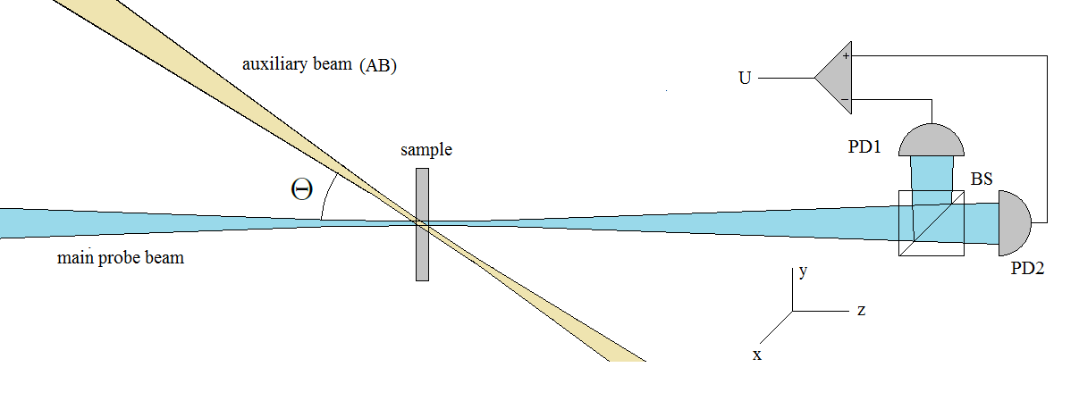 Figure 1
Peer Reviews
No public reviews on file for this paper yet. If you reviewed it on a platform where reviews are public (OpenReview, ICLR, NeurIPS, ICML), you can paste yours below so the community can read it here.
Videos
No videos yet. Explain this paper in a talk, walkthrough, or lecture? Add one.
Light scattering in the medium with fluctuating gyrotropy: application to spin noise spectroscopy
G. G. Kozlov, I. I. Ryzhov, V. S. Zapasskii
Abstract
The spin noise signal in the Faraday-rotation-based detection technique can be considered equally correctly either as a manifestation of the spin-flip Raman effect or as a result of light scattering in the medium with fluctuating gyrotropy. In this paper, we present rigorous description of the signal formation process upon heterodyning of the field scattered due to fluctuating gyrotropy. Along with conventional single-beam experimental arrangement, we consider here a more complicated, but more informative, two-beam configuration that implies the use of an auxiliary light beam passing through the same scattering volume and delivering additional scattered field to the detector. We show that the signal in the spin noise spectroscopy arising due to heterodyning of the scattered field is formed only by the scattered field components whose wave vectors coincide with those of the probe beam. Therefore, in principle, the detected signal in spin noise spectroscopy can be increased by increasing overlap of the two fields in the momentum space. We also show that, in the two-beam geometry, contribution of the auxiliary (tilted) beam to the detected signal is represented by Fourier transform of the gyrotropy relief at the difference of two wave vectors. This effect can be used to study spin correlations by means of noise spectroscopy.
Introduction
The spin noise spectroscopy (SNS), first realized in [1], has turned nowadays into a powerful method of studying magnetic resonance and spin dynamics in atomic and semiconductor systems (see, e.g., [2, 3, 4] . The most fascinating results of application of the SNS with the greatest progress in sensitivity of the measurements were achieved in physics of semiconductor structures, where the novel technique has allowed one not only to considerably move ahead in the magnetic resonance spectroscopy, but also to discover fundamentally new opportunities of research. Specifically, it has been established that optical spectroscopy of spin noise (that implies measuring wavelength dependence of the spin noise power) makes it possible to decipher inner structure of optical transitions [5]. Correlation nature of the SNS allowed one to realize, on its basis, a sort of pump-probe spectroscopy [6]. Effective dependence of the spin-noise signal on the light-power density (on the beam cross section) was used to demonstrate the SNS-based 3D tomography [8, 9]. Due to high sensitivity of the SNS, it appeared possible to detect magnetic resonance of quasi-free carriers in a single quantum well 20 nm thick [10], to observe the spin-noise spectrum of a single hole spin in a quantum dot [11], and to realize magnetometry of local magnetic fields (including field of polarized nuclei) in a semiconductor [12, 13]. Due to these remarkable capabilities of the new technique, it acquired a great popularity during the last decade.
At the same time, fundamental mechanism underlying the effect of magnetic resonance in the Faraday rotation noise spectrum remains so far, to a considerable extent, unexplored. Theoretically, it has been shown in 1983 [14] that this effect is closely related to the spin-flip Raman scattering, and the detected signal of magnetic resonance is the result of heterodyning of the scattered light (with shifted frequency), with the local oscillator provided by the probe laser beam. In this case, the standard experimental geometry we use in the conventional SNS may appear to be far from optimal. Indeed, we usually collect, on the photodetector, only the scattered light lying within the solid angle of the probe beam, whereas indicatrix of the Raman-scattered light may be fairly isotropic. It means that, in the standard experimental geometry, most part of the scattered light is lost. Therefore, it looks like the detected signal, in the SNS, can be considerably increased by collecting more efficiently the scattered light. Still, even if this simple picture is correct, it is not easy to correctly design the experimental setup to take advantage of the additional scattered field in full measure. First experiments carried out in this direction [15] and our preliminary analysis of the problem have shown that favourable solution of this experimental task can be achieved only with allowance for all the factors affecting the heterodyning process (wave fronts of the reference and scattered waves, shape of the beam, volume of the scattering medium, shape and dimensions of the photosensitive surface, correlation properties of the gyrotropy, etc. ). Actually, this problem, which we consider to be fundamental for the SNS method, is rather complicated and needs to be analyzed carefully and rigorously, with the results of the treatment applicable to real experimental conditions. In our opinion, computational details of such a treatment and prticularities of used apprpximations are also highly important.
In this paper, we present such a treatment for a focused Gaussian probe beam propagating through the medium with fluctuating gyrotropy and analyze in detail mechanism of the intensity-noise signal formation due to heterodyning of the scattered field on the detector. We also propose a two-beam experimental arrangement, with the auxiliary light beam tilted with respect to the probe, that makes it possible to get information about the spatiotemporal correlation function of gyrotropy of the studied system (remind that in conventional SNS only spatially averaged temporal correlation function is revealed).
The paper is organized as follows. In Section 1, for completeness of the narrative, we present a brief explanation of what is the Gaussian beam and introduce a model of the polarimetric detector used in our further analysis. We show here that the detected signal in SNS is contributed only by the scattered field that, in the momentu, space, coincides with that of the probe. In Section 2, we present basics of the single-scattering theory, apply it to the medium with gyrotropy randomly modulated in space, and calculate the observed polarimetric signal. In Sections 3 and 4, we calculate the noise signal observed in the two-beam configuration, when the auxiliary beam propagating though the medium at some angle to the main probe beam does not hit the detector and contributes to the signal only by its scattered field. We show that the spin-noise signal, under these conditions, is proportional to the Fourier component of the spatial correlation function of gyrotropy at spatial frequency equal to difference between the two wave vectors. In Section 5, we present calculations for the model of independent paramagnetic particles (spins) and show that the signal produced by the auxiliary tilted beam is of the same order of magnitude as the one produced by the main probe and, hence, can be easily detected using the same experimental setup.
1 Detecting polarimetric signal in a confined laser beam
In the simplest version of the light-scattering problem, the probe beam can be taken in the form of a plane wave. However, in the SNS experiments under consideration, when two light beams are supposed to be used, with their spatial localization being of crucial importance, this approximation proves to be inappropriate. So, we will treat Gaussian beams whose electric fields are defined by the expression
[TABLE]
where , ( is the optical frequency and is the speed of light), – beam intensity, and
[TABLE]
Field (1) satisfies Maxwell’s equations and represents the beam propagating in the plane at the angle with respect to axis ( is assumed to be snall) and polarized mostly in -direction. The parameter defines the -level half width of the beam waist by relationship . should be greater than the wavelength . In our estimations, we accept m and m.
In the SNS experiments, we detect small fluctuations of the optical field polarization, and, therefore, to calculate correctly the SNS signal, we have to specify the model of polarimetric detector. We suppose the detector to be comprised of two photodiodes PD1 and PD2 (Fig.1) arranged in two arms of the polarization beamsplitter (BS). The output signal is obtained by subtracting photocurrents of the two photodiodes and (to within some unimportant factors) are given by the expression
[TABLE]
where are the and components of the complex input optical field , are the dimensions of sensitive areas of the photodiodes along the and directions. We ascribe physical sense to real part of the complex optical field and, as seen from Eq. (2), the output signal represents the difference between intensities of the input optical field in the and polarizations integrated over sensitive areas of the photodiodes and averaged over the optical period .
In our case, the input optical field can be presented as a sum of the probe field (Re ) and the field (Re ) arising due to scattering of the probe beam by the sample with spatially fluctuating gyrotropy. Then, the first-order (with respect to ) contribution to the polarimetric signal can be written as
[TABLE]
This formula shows that the observed signal can be thought of as a result of heterodyning (mixing) of the unperturbed probe field with the field of scattering . Equation (3) also shows that , for sufficiently large dimensions of the detector (), polarimetric signal represents projection of the scattered field (in the momentum space) onto the field of the probe beam. This means, in turn, that this signal is controlled by the fraction of the scattered field whose distribution in space, to a certain extent, reproduces the field of the probe beam. Specifically, when the probe field represents a plane wave with the wave vector , and the scattered field can be presented by a superposition of the plane waves , the signal appears to be proportional to the component of the scattered field at the spatial frequency : .
Let us now calculate the scattered field .
2 Polarimetric signal in the medium with fluctuating gyrotropy
In this section, we consider scattering of a monochromatic light beam by the medium with randomly inhomogeneous (spatially fluctuating) gyrotropy. In this case, polarization of the medium can be expressed through the electric field by the expression
[TABLE]
where is the spatially dependent gyration vector. At this stage of our treatment, we assume the gyration vector to be time-independent. Then, Maxwell’s equations for the electromagnetic field in the medium can be reduced to the form:
[TABLE]
We will search for solution of this equation in the form of series in powers of . The zero order term represents the probe beam field which we consider to be known. The first order term corresponds to the single-scattering approximation which is sufficient for our consideration. This term satisfies the equation
[TABLE]
Solution of this equation can be expressed in terms of Green’s function of the Helmholtz equation :
[TABLE]
Let the sample (we call “sample” the region where is nonzero) be placed in the vicinity of the origin of our coordinate system . Let the photosensitive surface of the polarimetric detector be parallel to the plane and the detector itself be set at , with being large compared with the sample dimensions. Then, as seen from Eq. (7), the scattered field can be presented as a sum of two contributions:
[TABLE]
[TABLE]
[TABLE]
We will concentrate on calculating the part of the scattered field because, in what follows, we will need this field at small scattering angles and, in this case, as it can be directly checked, only is of importance.
We take the probe beam in the form of Eq. (1) at , with the angle specifying beam polarization in the plane. Then, the probe field acquires the form
[TABLE]
We need this field in two substantially separated spatial regions: firstly, in Eq.(3) at large values of and, secondly, in Eq.(8) at relatively small values of within the sample. Calculation for shows that the field entering Eq.(3) has the form
[TABLE]
While deriving these expressions, we assumed that ( is the Rayleigh length). To calculate the scattered field by Eq. (8), one needs the field (9) at . In this limit, Eq. (9) can be simplified:
[TABLE]
Using this relationship, one can calculate the scattered field (8) and obtain, for real parts of and entering Eq. (3), the following expressions:
[TABLE]
Using Eq. (3) and explicit expressions (10) and (12) for the probe and scattered fields, we can calculate the polarimetric signal. While averaging the product over the optical period, we come to the integral
[TABLE]
[TABLE]
The same is obtained for . Now, Eq. (3) gives
[TABLE]
[TABLE]
with and . The external integration over runs over the detector sensitive area, and, therefore, . We assume that dimensions of the detector exceed the size of the probe beam spot at the detector (see Eq. (10)). Then, and can be estimated as . The internal integration runs over the irradiated volume of the sample. For this reason and is of the order of the sample length . Taking into account that , we obtain the following expansion for the factor :
[TABLE]
Note that the term vanishes. Further estimates show that the term can be omitted because in our case and, finally, we have
[TABLE]
Using this formula, we can evaluate the product of the cosine functions in (13) as
[TABLE]
As was mentioned above, the detector dimensions are assumed to be greater than the size of the probe beam spot: . This allows one to extend integration over the detector surface in (13) to infinity: and to calculate all integrals using the formula
[TABLE]
For example, the integral with cosine function in Eq.(16) (we denote it ) can be calculated as follows:
[TABLE]
[TABLE]
[TABLE]
[TABLE]
Substituting (18) into (13), we obtain the following expression for the polarimetric signal:
[TABLE]
Remind that this formula is valid if the sample length is smaller than the Rayleigh length, (see definition of the Rayleigh length after Eq. (10)) and the probe beam spot is smaller than the detector photosensitive area, . It is seen from Eq. (19) that the polarimetric signal is, in fact, proportional to -component of the gyration averaged over irradiated volume of the sample, as is usually implied intuitively.
Equation (19) allows one to obtain the expression for the magnetization noise power spectrum observed in the SNS. In this case, is proportional to instantaneous spontaneous magnetization of the sample randomly fluctuating both in space, and in time. If characteristic frequencies of this field are much lower than the optical frequency , one can use Eq. (19) for calculating the random polarimetric signal by substituting . The noise power spectrum is defined as Fourier transform of correlation function of the polarimetric signal. Using Eq. (19), the noise power spectrum can be expressed in terms of the spatiotemporal correlation function of the gyrotropy :
[TABLE]
[TABLE]
To calculate the correlation function entering Eq. (20), one should specify a particular model of the gyratropic medium. The example of such a model (the model of independent paramagnetic atoms with fluctuating magnetization) will be described in Section 5. In the next section, we will calculate the plarimetric signal produced by an auxiliary tilted beam that produces a scattered field but does not irradiate the detector (see Fig. 1).
3 Detecting scattered field of a tilted beam
Let the sample be illuminated by an auxiliary light beam (AB) propagating at the angle with respect to the main probe beam (Fig. (1)). Note that AB does not hit the detector, but the scattered field of this beam may provide additional contribution to the detected polarimetric signal, and our goal now is to calculate value of this contribution.
The calculation can be performed in the same way as in the previous section with the following changes. The scattered field is calculated using Eq. (8) with the field replaced by , where represents the field of the auxiliary (tilted) beam. The field can be obtained by rotating by the angle around the axis parallel to the direction of polarization of the probe beam 111Thus, polarizations of the tilted and the probe beams are the same:
[TABLE]
Here, the matrix is defined as
[TABLE]
[TABLE]
Therefore, the field is defined by the expression
[TABLE]
where
[TABLE]
with . We denote by intensity of the AB and take into account its possible spatial shift . Substituting (23) into Eq. (8) instead of , one can obtain the following expression for the scattered field produced by AB:
[TABLE]
where , and , with the functions , , defined by Eq. (24) with substitution . This formula has the same sense as Eq. (12); for clarity we supply components of the scattered field by superscript . Taking into account this replacements, one can get the relationship for polarimetric signal produced by the AB (instead of Eq. (13))
[TABLE]
[TABLE]
Calculation of intergrals can be made as in the previous section, and the final result for the polarimetric signal produced by the AB is:
[TABLE]
where
[TABLE]
One can see that is proportional to overlap of the two beams and vanishes at large shifts . The trigonometric factor , in fact, singles out harmonic of the gyrotropy with the spatial frequency equal to difference between the wave vectors of the two beams. Total signal in the presence of two beams is the sum of (19) and (27): . Remind that the angle should not be too large; otherwise, one should take into account the component in Eq. (8).
4 Noise signal in the two-beam configuration
The noise signal produced by the two beams in the configuration of Fig. 1 is calculated as Fourier transform of correlation function of the total polarimetric signal . It consists of 3 terms:
[TABLE]
Using Eqs. (19) and (27), one can write the expressions for each of them. The first term has been already calculated and is given by Eq. (20). For the correlator entering the last term, we have
[TABLE]
[TABLE]
where and are defined by Eq. (28)
[TABLE]
are similar functions of .
Finally, the cross correlator can be written as
[TABLE]
[TABLE]
Consider now physical sense of different factors entering Eqs.(20), (30), and (32).
**Exponential factor ** reduces the region of integration down to the region of overlapping of the two beams. If is not too large and , this region is close to “the beam volume within the sample”. In this case, the exponential factor can be calculated at . Note that it is rather difficult to satisfy the condition in a real experiment. For this reason, the overlapping factor may considerably reduce contribution of the AB to the polarimetric signal.
**Trigonometric factor ** at small angles is controlled by the difference between wave vectors of the two beams because the cosine argument can be evaluated as .
**Correlation function ** is determined by particular model of the gyrotropic medium. For homogeneous media, it depends on the difference of the spatial arguments. For the model of independent spins, described below
Thus, the integrals entering Eqs.(20), (30), and (32) can be calculated for any particular model of the gyrotropic medium. In the next section, we will present calculations for the model of independent paramagnetic particles (spins). Still, the following general remark should be made. Let the beam waist and the sample length be much greater than the gyrotropy correlation radius and spatial period related to the difference of wave vectors of the two beams: . Then, one can substitute variables in the integrals entering Eqs.(20), (30), and (32) in the following way: and take advantage of the fact that the correlator depends on difference of its arguments:
[TABLE]
Then, the integral over in Eq. (20) can be estimated as the average of over irradiated volume of the sample . The integration over gives this volume itself, and we obtain
[TABLE]
[TABLE]
Here, we denote the cross section area of the beam by and take into account that and that irradiated volume of the sample is , where is the sample length. We come to the known result that the noise power signal is proportional to the sample length and inversely proportional to the beam cross section [1, 16, 17].
The correlation function Eq.(30) can be estimated in a similar way. If is not too large, then the arguments of the cosine functions can be evaluated as and . Therefore, one can represent the product of the cosine functions in Eq.(30) as
[TABLE]
[TABLE]
Note that the difference between the wave vector of the two beams for small has only and components: . Therefore, this relationship after substitution of variables takes the form
[TABLE]
Remind that our treatment is valid when is large enough (). In this case, the integral , and we come to conclusion that the correlation function Eq. (30) can be estimated as follows
[TABLE]
[TABLE]
Thus, contribution of the auxiliary tilted beam (AB) to the noise signal is proportional to Fourier transform of the correlation function of gyrotropy at spatial frequency equal to difference of the wave vectors of the two beams ().
Therefore, by measuring dependence of the noise signal, in the two-beam configuration, on the angle between the beams (in fact, on ) and using the inverse Fourier transform, one can restore spatial dependence of the gyrotropy correlation function . Recall that in the conventional spin noise spectroscopy, only temporal dependence of this correlation function averaged over the irradiated volume of the sample is revealed.
Similarly, it can be shown that, under these conditions, contribution of the cross correlator Eq. (32) is relatively small.
5 The model of independent spins
In this model, the random field of gyrotropy has the form
[TABLE]
thus corresponding to paramagnetic particles (spins) randomly distributed over the volume of the medium with some average density , where is the total volume of the system. We assume that is proportional to -component of magnetization of the -th particle. The polarimetric signal can be calculated using Eq.(19):
[TABLE]
Let us calculate polarimetric signal for the sample in which all magnetizations are constant and the same: const. This corresponds to a paramagnet in a high magnetic field at low temperature. In this case, Eq. (37) gives
[TABLE]
We will see below that the quantity provides us a convenient scale. Let us now consider the gyrotropic medium with the quantities changing randomly in a stationary way with the correlation function (should be distinguished from the spatiotemporal correlation function of Eq. (33)) and calculate, for this model, the noise power spectrum using Eq. (20). We have
[TABLE]
and, consequently,
[TABLE]
If we accept for beam area the expression , then . Taking into account Eq. (38), we obtain the expression for noise power spectrum
[TABLE]
Note that is the number of spins in the irradiated volume of the sample.
In the simplest case, each paramagnetic particle of the gyrotropic medium can be associated with the effective spin 1/2. Then, the total magnetization can be expressed as: (here, is the effective -factor and is the Bohr magneton). In the presence of the transverse magnetic field , the correlator can be calculated using the following chain of relationships:
[TABLE]
Here, is the density matrix of the two-level system representing our effective spin 1/2. If the temperature is high enough (), the density matrix can be taken constant, ( is the unit matrix), and we obtain
[TABLE]
[TABLE]
We introduce phenomenologically the transverse relaxation time . So, for the noise power spectrum we have
[TABLE]
The root-mean-square value of the polarimetric noise is given by the relationship
[TABLE]
In a similar way, one can calculate the power spectrum of the polarimetric noise in the presence of the auxiliary beam AB. Using Eq. (38) for the correlation function and Eqs. (20), (30), and (32), we obtain:
[TABLE]
If m, , and m, the exponential factors can be omitted, and simplified expressions for the correlation function and the noise power spectrum acquire the form
[TABLE]
[TABLE]
It is seen from Eq. (48) that if , then switching the axiliary beam on leads to 50 increase of the noise power and, therefore, can be easily observed. Note once again that we assumed complete overlapping of the two beams. Therefore, the contribution of the auxiliary beam to the noise power spectrum in real experiments, when this is not the case, may be somewhat smaller.
The above treatment was performed for the case of absence of any spatial correlation in the field of gyrotropy. The rfesult of this assumption is the absence of any dependence of the noise signal on the angle (at small ). In the presence of spatial correlation of the gyrotropy, the noise signal will decrease with (with increasing ). Specifically, if the noise signal decreases, say, by a factor of 2 at an angle of , then the correlation radius of the gyration field can be estimated as .
Conclusion
The main goal of the paper was to understand deeper the role and properties of the scattered field underlying signal formation in the Faraday-rotation-based spin noise spectroscopy. The sample with fluctuating spins is considered as an optical medium with its gyrotropy fluctuating both in time and in space. The noise signal arising due to heterodyning of the light scattering by the inhomogeneous medium is calculated for a focused Gaussian beam in the single-scattering approximation. We show that, in real experiments, only a small fraction of the scattered field contributes to the detected signal, namely, onle components of the scattered field that overlap with those of the probe beam in the momentum space. Therefore, a more efficient use of the scattered field, in spin noise spectroscopy, can be achieved by increasing this overlap in proper optical arrangements. Our calculations confirm the common assumption that the noise signal, in the conventional geometry of spin noise spectroscopy, is proportional to the sample’s gyrotropy spatially averaged over the irradiated volume. We also consider a two-beam experimental arrangement in which properties of the scattered light field are revealed in a much more pronounced way. We show that the signal produced by the auxiliary light beam tilted with respect to the probe is proportional to Fourier transform of the gyrotropy at spatial frequency equal to difference of the wave vectors of two beams. Accordingly, in the presence of spatial correlation of the gyrotropy field, Fourier components at higher spatial frequencies will appear to be suppressed, and contribution of the auxiliary beam into the noise signal at larger angles between the beams will decrease. This effect can be used to investigate spatial correlation of spins in spin noise spectroscopy. The results of rigorous solution of the problem are presented here for the case of spatially uncorrelated gyrotropy with, correspondingly, ”white” spatial spectrum of the gyrotropy fluctuations. The results of this study are important from the viewpoint of fundamental physics of signal formation in the spin noise spectroscopy and , at the same time, may be useful for increasing sensitivity of the spin-noise technique.
The reference list from the paper itself. Each links out to its DOI / PubMed record.
- 1[1] E.B.Aleksandrov and V.S.Zapasskii, “Magnetic resonance in the Faraday rotation noise spectrum”, JETP, 54, 64 (1981)
- 2[2] V. S. Zapasskii, Adv. Opt. Photon., 5, 131 (2013)
- 3[3] G.M.Müller, M.Oestreich, M.Römer, and J.Hübner, “Semiconductor spin noise spectroscopy: Fundamentals, accomplishments, and challenges” Physics E, 43, 569 (2010)
- 4[4] N A Sinitsyn 1 and Yu V Pershin, Rep. Prog. Phys. 79 106501 (2016)
- 5[5] V. S. Zapasskii, A. Greilich, S. A. Crooker, Yan Li, G. G. Kozlov, D. R. Yakovlev, D. Reuter, A. D. Wieck, and M. Bayer, “Optical spectroscopy of spin noise,” Phys. Rev. Lett., vol. 110, 176601 (2013)
- 6[6] Luyi Yang, P. Glasenapp, A.Greilich, D. Reuter, A.D. Wieck, D.R.Yakovlev, M. Bayer and S.A.Crooker ”Two color spin noise spectroscopy and fluctuation correlations reveal homogeneous linewidth wthin quantum-dot ensembles” Nat. Commun. 5 4949 (2014)
- 7[7] M. Oestreich, M. Röemer, R. G. Haug, and D. Hagele, Phys. Rev. Lett., 95, 216603 (2005)
- 8[8] M. Römer, J. Hübner, and M. Oestreich, “Spatially resolved doping concentration measurement in semiconductors via spin noise spectroscopy,” Appl. Phys. Lett. 94, 112105 (2009).