The pseudoscalar meson electromagnetic form factor at high $Q^2$ from full lattice QCD
J. Koponen, A. C. Zimermmane-Santos, C. T. H. Davies, G. P. Lepage, A., T. Lytle

TL;DR
This study uses full lattice QCD to accurately determine the electromagnetic form factor of a light pseudoscalar meson up to high momentum transfer, providing insights into the transition from non-perturbative to perturbative QCD regimes.
Contribution
First lattice QCD calculation of the pseudoscalar meson form factor up to 6 GeV^2 including sea quarks, controlling discretisation and sea quark effects.
Findings
Q^2F(Q^2) becomes flat between 2 and 6 GeV^2
Values exceed perturbative QCD expectations at high Q^2
Results applicable to pion form factor studies
Abstract
We give an accurate determination of the vector (electromagnetic) form factor, , for a light pseudoscalar meson up to squared momentum transfer values of 6 for the first time from full lattice QCD, including , , and quarks in the sea at multiple values of the lattice spacing. Our results show good control of lattice discretisation and sea quark mass effects. We study a pseudoscalar meson made of valence quarks but the qualitative picture obtained applies also to the meson, relevant to upcoming experiments at Jefferson Lab. We find that becomes flat in the region between of 2 and 6 , with a value well above that of the asymptotic perturbative QCD expectation, but well below that of the vector-meson dominance pole form appropriate to low values. Our calculations show that we can…
Click any figure to enlarge with its caption.
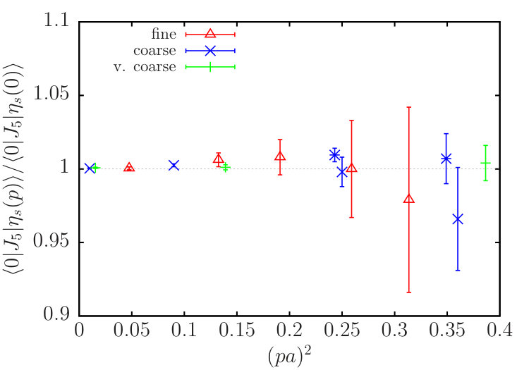 Figure 1
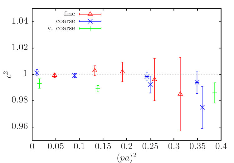 Figure 2
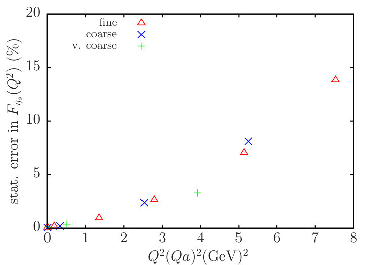 Figure 3
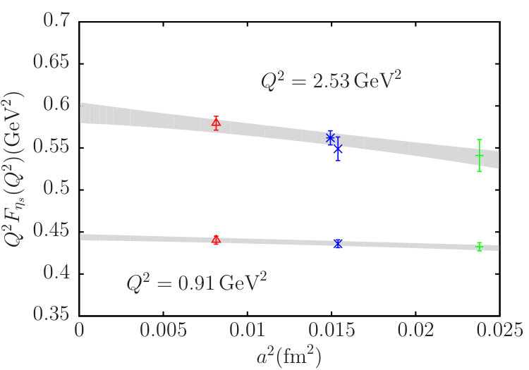 Figure 4
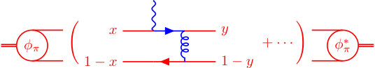 Figure 5
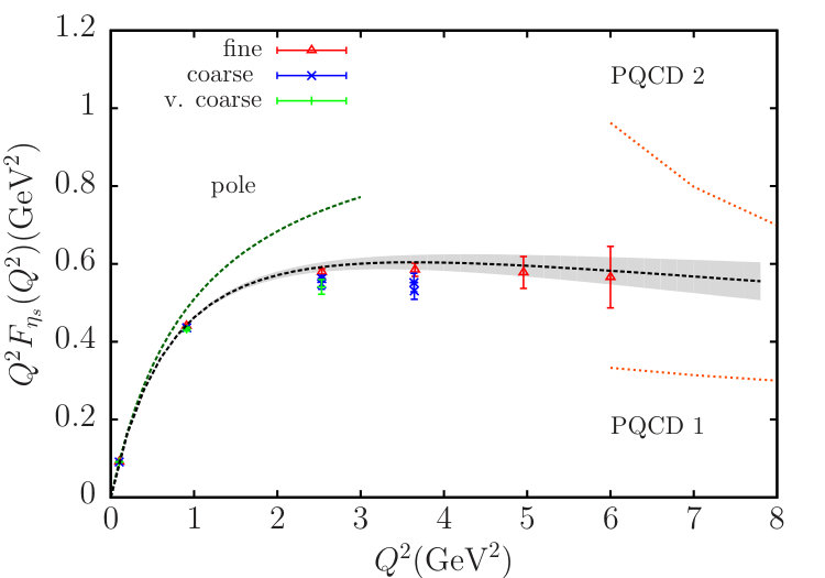 Figure 6
| Set | ||||||||||
|---|---|---|---|---|---|---|---|---|---|---|
| 1 | 5.8 | 1.1119(10) | 0.0130 | 0.0650 | 0.838 | 0.0705 | 0.54028(15) | 0.1243,0.3730,0.6217 | 1020 | |
| 2 | 6.0 | 1.3826(11) | 0.0102 | 0.0509 | 0.635 | 0.0541 | 0.43135(9) | 0.1,0.3,0.5,0.6( 4 dirns) | 1053 | |
| 3 | 6.0 | 1.4029(9) | 0.00507 | 0.0507 | 0.628 | 0.0533 | 0.42636(6) | 0.493,0.591 | 1000 | |
| 4 | 6.3 | 1.9006(20) | 0.0074 | 0.037 | 0.44 | 0.0376 | 0.31389(7) | 0.0728,0.218,0.364,0.437,0.509,0.56 | 1008 |
| Set | ||||||||||||
|---|---|---|---|---|---|---|---|---|---|---|---|---|
| 1 | 0.1012 | 0.9003(9) | 0.9109 | 0.4747(18) | 2.531 | 0.2138(70) | ||||||
| 2 | 0.1012 | 0.9009(5) | 0.9111 | 0.4786(10) | 2.531 | 0.2170(51) | 3.644 | 0.1456(59) | ||||
| 3 | 2.533 | 0.2219(23) | 3.640 | 0.1517(65) | ||||||||
| 4 | 0.1014 | 0.9014(6) | 0.9091 | 0.4843(9) | 2.535 | 0.2286(22) | 3.653 | 0.1602(42) | 4.956 | 0.1167(82) | 5.999 | 0.094(13) |
| Set | |
|---|---|
| 1 | 1.3892(15) |
| 2 | 1.3218(7) |
| 3 | 1.3179(7) |
| 4 | 1.2516(9) |
Peer Reviews
No public reviews on file for this paper yet. If you reviewed it on a platform where reviews are public (OpenReview, ICLR, NeurIPS, ICML), you can paste yours below so the community can read it here.
Videos
No videos yet. Explain this paper in a talk, walkthrough, or lecture? Add one.
HPQCD collaboration
The pseudoscalar meson electromagnetic form factor at high from full lattice QCD
J. Koponen
SUPA, School of Physics and Astronomy, University of Glasgow, Glasgow, G12 8QQ, UK
INFN, Sezione di Tor Vergata, Dipartimento di Fisica, Università di Roma Tor Vergata, Via della Ricerca Scientifica 1, I-00133 Roma, Italy
A. C. Zimermmane-Santos
SUPA, School of Physics and Astronomy, University of Glasgow, Glasgow, G12 8QQ, UK
São Carlos Institute of Physics, University of São Paulo, PO Box 369, 13560-970, São Carlos, SP, Brazil
C. T. H. Davies
SUPA, School of Physics and Astronomy, University of Glasgow, Glasgow, G12 8QQ, UK
G. P. Lepage
Laboratory for Elementary-Particle Physics, Cornell University, Ithaca, New York 14853, USA
A. T. Lytle
SUPA, School of Physics and Astronomy, University of Glasgow, Glasgow, G12 8QQ, UK http://www.physics.gla.ac.uk/HPQCD
Abstract
We give an accurate determination of the vector (electromagnetic) form factor, , for a light pseudoscalar meson up to squared momentum transfer values of 6 for the first time from full lattice QCD, including , , and quarks in the sea at multiple values of the lattice spacing. Our results show good control of lattice discretisation and sea quark mass effects. We study a pseudoscalar meson made of valence quarks but the qualitative picture obtained applies also to the meson, relevant to upcoming experiments at Jefferson Lab. We find that becomes flat in the region between of 2 and 6 , with a value well above that of the asymptotic perturbative QCD expectation, but well below that of the vector-meson dominance pole form appropriate to low values. Our calculations show that we can reach higher values in future to shed further light on where the perturbative QCD result emerges.
I Introduction
Hitting one constituent of a bound state with a photon initiates a complicated process if the bound state is not to fall apart. The momentum gained must be redistributed between all the constituents so that the whole convoy can slew round into the new direction. A price is paid in terms of a reduced interaction strength between the photon and the bound state and this is known as the electromagnetic form factor - a function of the square of the (space-like) 4-momentum, , transferred from initial to final state. When the bound state is a hadron, and held together by the strong interaction, the determination of the form factor becomes a case study for our understanding of Quantum Chromodynamics (QCD) as a function of . Both experimental measurement Huber et al. (http://www.jlab.org/exp_prog/proposals/06/PR12-06-101.pdf) and theoretical calculation are important. As we show here, lattice QCD, now including a realistic QCD vacuum Davies et al. (2004), can provide key theoretical results.
The meson is one of the simplest hadrons, with a valence quark and antiquark chosen from . At small values of squared momentum transfer, up to 0.25 , its electromagnetic form factor, , has been measured directly by scattering from atomic electrons Amendolia et al. (1986). The form factor can be fitted to a simple pole form in this region and the pole mass (close to that of the vector, Frazer and Fulco (1959)) can be related to the r.m.s. electric charge radius. Lattice QCD calculations of the form factor at small values of Brommel et al. (2007); Boyle et al. (2008); Frezzotti et al. (2009); Aoki et al. (2009); Nguyen et al. (2011); Brandt et al. (2013); Aoki et al. (2016); Koponen et al. (2016) give a theoretical determination that agrees well with experiment.
At the other extreme of the range, very large values, a perturbative QCD treatment of the electromagnetic form factor becomes possible because the process in which the hard photon scatters from the quark or antiquark factorises from the distribution amplitudes which describe the quark-antiquark configuration in the meson Lepage and Brodsky (1979, 1980). The hard scattering amplitude is inversely proportional to and can be treated perturbatively in QCD because a high photon must be accompanied by a high momentum gluon exchange between the meson constituents (see Figure 1). The asymptotic perturbative QCD prediction, as , is very simple because the distribution amplitude can be normalised using the pion decay constant ( = 130.4 MeV) Farrar and Jackson (1979); Efremov and Radyushkin (1980); Lepage and Brodsky (1979). This gives
[TABLE]
but this is not expected to be valid until values of tens of are reached Lepage and Brodsky (1980). Meanwhile, the approximately constant value of from Eq. (1) is numerically very different from the results and trend seen at small . This means that there is a large gap to be filled in our understanding, extending to relatively high values Department of Energy Nuclear Science Advisory Committee (http://science.energy.gov/np/nsac).
For of a few an indirect experimental method must be used to determine with scattering of electrons from the pion cloud around a proton Brauel et al. (1977, 1979); Ackermann et al. (1978). The most recent results from Jefferson Lab Volmer et al. (2001); Tadevosyan et al. (2007); Horn et al. (2006); Blok et al. (2008); Huber et al. (2008) have reached but extension to is foreseen Huber et al. (http://www.jlab.org/exp_prog/proposals/06/PR12-06-101.pdf), starting in 2018, as a key experiment (E12-06-101) for the 12 GeV upgrade.
This is also a region in which lattice QCD can be used to calculate the meson electromagnetic form factor directly, as we demonstrate here. The method is straightforward, and the same for all values. To reach higher values the participating meson 3-momentum and therefore energy must be increased. Both statistical errors and systematic errors from discretisation effects will then increase, so it is important to have a high statistics calculation in a quark formalism with small discretisation errors. Previous lattice QCD calculations (see Brandt (2013) for a review) that include , and quarks in the sea Bonnet et al. (2005); Lin and Cohen (2011); Chambers et al. (2017) have concentrated on having many values for different heavy pion masses at one value of the lattice spacing. This has enabled studies of pion mass dependence but precluded taking a continuum limit. See also Brommel et al. (2007) for a more extensive calculation but including only and quarks in the sea.
Here we are able to reach values of of 6 with an accuracy of 10% by performing a high statistics calculation at a number of well-separated values. Instead of studying mesons we work consistently with a ‘pseudopion’, a pseudoscalar meson made of valence quarks (denoted ), accurately tuned Chakraborty et al. (2015) on full QCD (with , , and quarks in the sea) ensembles of gluon field configurations at three values of the lattice spacing and two values of the sea quark masses. We work with quarks because it is numerically much faster to accumulate high statistics for a precise result, little dependence on the sea mass is expected and finite-volume effects are negligible Dowdall et al. (2013). We use the Breit frame where the initial and final mesons have opposite spatial momenta, and is maximized for a given . By working at values of the lattice spacing that range over a factor of 1.7 we are able to show that discretisation errors are small for our formalism, even at relatively large , and to extrapolate to the zero lattice spacing continuum limit.
Our mesons are qualitatively very similar to mesons for the purposes of this study, because the quark is light compared to QCD scales. Both the small- pole form and very high perturbative QCD results for the form factor can be readily determined and thus our lattice QCD results provide a clear comparison to these two pictures in the region of . In future we can extend this work to even higher and also calculate other form factors, inaccessible to experiment, which can be compared to perturbative QCD to understand the range in which it becomes valid. Most importantly, our results show the way to accurate predictions for from lattice QCD for the upcoming Jefferson Lab experiments Huber et al. (http://www.jlab.org/exp_prog/proposals/06/PR12-06-101.pdf).
II Lattice QCD Calculation
The electromagnetic, or vector, form factor for a pseudoscalar meson, , is determined from
[TABLE]
where is a vector current coupling to the photon. Here we use the temporal component of and so that the right-hand side of eq. (2) becomes with .
The matrix element is determined in lattice QCD by combining information from meson ‘2-point’ and ‘3-point’ functions DeGrand and DeTar (2006). 2-point functions tie together quark and antiquark propagators for a correlation function that creates a hadron at time 0 and destroys it at time . 3-point functions combine 3 propagators so that a meson is created at time 0, its quark (or antiquark) carrying momentum interacts with a photon at time and is scattered into , with the meson being destroyed at time 111 Charge-conjugation symmetry means that quark-line disconnected diagrams vanish in this case Draper et al. (1989).. We fit the -, - and -dependence of the 2- and 3-point results (averaged over the gluon field configurations in an ensemble and including all results above a of 3) simultaneously to a multi-exponential form in Euclidean time that includes the set of possible mesons made from this valence quark and antiquark Koponen et al. (2016). This enables us to isolate the matrix element for the ground-state, lightest, meson and relate it to the required form factor, whilst making sure that systematic effects from the presence of higher mass states in the correlator are taken into account. We can normalise the form factor by the electric charge conservation requirement that .
We use the Highly Improved Staggered Quark (HISQ) formalism designed Follana et al. (2007), and shown Follana et al. (2008); Davies et al. (2010); Donald et al. (2012); Dowdall et al. (2013), to have very small discretisation errors from the lattice spacing. We work on gluon field configurations generated by the MILC collaboration Bazavov et al. (2010, 2013) that include HISQ , , and quarks in the sea and also have a highly-improved gluon action Hart et al. (2009). On these configurations we study the . In lattice QCD we can prevent this particle from mixing with other isospin zero mesons and then its properties can be well determined Dowdall et al. (2013) and it behaves as a pseudopion; its mass is 688.5(2.2) MeV and decay constant 181.14(55) MeV. Here we determine its vector form factor as a function of .
Table 1 gives the parameters of the gluon field configurations we use, with lattice spacing varying from 0.15 fm to 0.09 fm and quark mass either twice or five times the physical value, corresponding to 216 or 304 MeV. We tune the valence quark mass on each ensemble to obtain the correct mass Chakraborty et al. (2015). We calculate 2-point functions with a range of spatial momenta with magnitude in lattice units up to 0.62, given in Table 1. These are implemented by using the ‘twisted boundary condition’ method Guadagnoli et al. (2006) and are chosen to be in the (1,1,1) direction to minimise discretisation effects. We use mesons made with the local (Goldstone) operator; in staggered quark parlance this corresponds to spin-taste Follana et al. (2007). For our 3-point correlation functions we use a 1-link temporal vector current with spin-taste .
We fit 2- and 3-point correlators simultaneously using Bayesian methods Lepage et al. (2002) to constrain fit parameters and determining the covariance between results at different values. The fit forms are Donald et al. (2012); Dowdall et al. (2013)
[TABLE]
The HISQ action gives opposite parity terms (o.p.t.) for mesons at non-zero momentum; they are similar to the terms given explicitly above but with factors of . The fit parameters are chosen to be the log of the ground-state energy, , and the log of energy differences between the (ordered) excitations, . For our kinematic set-up , with the ground-state to ground-state amplitude. The division by provides the normalisation of the lattice current. Results for the renormalisation factors inferred from are given in Appendix A.
We use priors of 800 400 MeV for the energy splitting between successive excitations and prior widths on amplitudes and of at least 2 times the ground-state value. We take results from fits that include 6 exponentials where ground-state values and their uncertainties have stabilised and we have checked that the prior widths have only a minor impact on these uncertainties. Although we are only interested in ground-state properties here, our correlators are precise enough to resolve the first excited state. We have checked that its mass (around 950 MeV above the ground-state) is in reasonable agreement with that for an excited state seen in Dudek et al. (2011). Note that we do not expect multi-meson (for example two kaon) energy levels to appear in our spectrum since the overlap of such states with our single meson operators is very small, being suppressed by the volume Dudek et al. (2010).
Results for the (ground-state) form factor are given in Table 2 and is plotted in Figure 2. Results on different ensembles lie close to each other, showing that effects from discretisation and different masses are very small. Tests of discretisation effects from studies of the meson energy and decay amplitudes as a function of spatial momentum are reported in Appendix B. We also show in Appendix B (see Figure 3) how statistical errors in the form factor grow as a function of and . It is in fact the statistical errors that provide a practical limit to how high in we can reach here for different values of the lattice spacing. Note that the finer lattices have larger reach in than the coarse.
To determine the form factor in the physical continuum limit we must extrapolate in the lattice spacing and sea quark mass. We do this using a model-independent parameterisation of the form factor now standard in both theory and experiment for semileptonic weak decays (see Hill (2006) for a recent review), mapping the domain of analyticity in onto the unit circle in . Since we can then perform a power series expansion in . We take Lee et al. (2015)
[TABLE]
where in our case is equal to . We choose the point that maps to to be , for simplicity; this gives of 0.46 at , well below 1. Rather than we work with , using . The product has reduced -dependence because is a good match to the form factor at small (the being the vector meson) and it has the correct dependence at large (but the wrong value: see Figure 2). To combine a -expansion with lattice QCD results we simply allow the coefficients in the expansion to have independent - and -dependence. Adapting the method from Koponen et al. (2013), we use the fit function
[TABLE]
Note that the lattice ‘data’ on the left-hand-side include correlations between results. The coefficients and account for dependence on the lattice spacing; we take 1 GeV to allow for and terms in . Independent coefficients at each order allow for -dependent discretisation effects. Only even powers of appear in the HISQ formalism and, because we work in the Breit frame with a fixed direction for , there is only one scale, , that can appear coupled with . Note that, by definition, there are no -independent discretisation errors. In Figure 6 of Appendix B we show results for at two values of plotted against the square of the lattice spacing, showing more explicitly the size of discretisation effects. We also show there how well the fit function of eq. (5) is able to reproduce the discretisation effects, including their dependence. accounts for the heavier-than-physical quark masses in the sea, using Chakraborty et al. (2015) and dividing by a factor of 10 to convert this to a suitable chiral perturbation theory expansion parameter. We take priors on the , and of 0.0(1.0) but on of 0.0(5), because leading errors are suppressed by in the HISQ formalism Follana et al. (2007). For the , the coefficients of the -expansion in the continuum and chiral limits, we take priors of 0.0(2.0), twice as conservative as the Bayesian probability function would suggest. We use ; adding higher terms has no impact and neither does adding terms.
Our fit has a of 0.3. The result at and physical quark masses (i.e. ) is plotted (converted back to space) in Figure 2 and shows little deviation from the results on the fine lattices. The fitted parameters and their covariance matrix are given in Appendix C.
III Discussion/Conclusions
Figure 2 shows the physical curve for determined from our results for . At small it is compared to the pole form, . Our results show that the physical curve peels away from the pole form at and then lies significantly below it. Also plotted in Figure 2, for , is the asymptotic perturbative QCD form (labelled PQCD 1) of Eq. (1), using instead of . For we have used at a scale of , since this is the momentum carried by the gluon when the quark and antiquark share the meson momentum equally. Our physical curve then lies significantly above this result at of 6 . We expect this qualitative picture of the physical curve to be true for the pion form factor to be determined in Jefferson Lab experiment E12-06-101 (the peeling away from the pole form is already apparent Huber et al. (2008)).
For non-asymptotic the leading perturbative QCD prediction is modified to Lepage and Brodsky (1979, 1980):
[TABLE]
where the sum is over even for a ‘symmetric’ meson (the used here or in the isospin limit). The , coefficients of an expansion in Gegenbauer polynomials, evolve logarithmically to zero as .
Lattice QCD calculations have been used to determine Arthur et al. (2011); Braun et al. (2015) and this changes the asymptotic prediction substantially in the region of around 10 . The calculation of yet higher order corrections is complicated by operator mixing Braun and Mueller (2008). It is important to understand the limitations of the perturbative QCD approach here, because the pion distribution amplitude inferred from is used in other calculations. They appear, for example, in light-cone sum rule calculations of the form factor at low for the exclusive weak decay to determine Khodjamirian et al. (2011); Bharucha (2012).
Figure 2 shows a curve (labelled PQCD 2) that uses a shape for the distribution amplitude at a scale where is the light-cone momentum fraction and is chosen to agree with lattice QCD results for for the Braun et al. (2015) (results indicate only weak quark mass-dependence, so this should be a good approximation). PQCD 2 is much higher than PQCD 1 at and shows stronger -dependence. To obtain a flatter curve in better agreement with our results would require a broader distribution amplitude and a higher scale for for less evolution. Such curves have been obtained for the in a recent Dyson-Schwinger approach Chang et al. (2013), and it would be interesting to see if it can reproduce our results for the . For this purpose we give the parameters for our continuum curve in Appendix C.
To extend our results to higher values of is possible on finer lattices where a given value of corresponds to a higher in GeV. A of 12 should be possible on ‘superfine’ lattices with 0.06 fm, and even 20 at 0.045 fm (‘ultrafine’). Lower statistics calculations have already been done on such lattices McNeile et al. (2010); McNeile et al. (2012a, b). See also Bali et al. (2016) for new methods to reduce uncertainties in calculations at high . The scalar form factor at high will give additional information since perturbative QCD Lepage and Brodsky (1979, 1980) predicts that this should fall more rapidly than .
Perturbative QCD (Eq. 6) predicts approximate scaling of the form factor with the square of the decay constant, and we can test this in lattice QCD as we reduce the pseudoscalar meson mass towards that of the . This scaling may set in before the -dependence becomes clearly that of perturbative QCD. If that is the case we can use our results here, rescaling by , to predict a value for in a flat region from of .
Acknowledgements. We are grateful to the MILC collaboration for the use of their gauge configurations and code and to B. Chakraborty and D. Hamilton for useful discussions. Our calculations were done on the Darwin Supercomputer as part of STFC’s DiRAC facility jointly funded by STFC, BIS and the Universities of Cambridge and Glasgow. This work was funded by a CNPq-Brazil scholarship, the National Science Foundation, the Royal Society, the Science and Technology Facilities Council and the Wolfson Foundation.
Appendix A Renormalisation factors
Table 3 gives the values of the vector current renormalisation factor, , for each ensemble inferred from electric charge conservation at . The vector current we use is a 1-link current in the time direction, made gauge-invariant by the includion of an APE-smeared gauge link. The values for show the expected qualitative behaviour, slowly falling towards 1 on finer lattices.
Appendix B Tests of statistical errors and discretisation effects
In Figure 3 we show how the statistical error in the form factor result grows with . The results from different lattice spacing values (for approximately the same number of configurations, spatial lattice volume and smallest value in physical units) appear to lie on a universal curve as a function of . The curve is approximately quadratic, showing that uncertainties degrade rapidly at large values. However the same can be reached with smaller on finer lattices, moving down the curve. The plot helps to predict the statistical accuracy that will be obtained from calculations on other lattices using the same (Breit) frame.
A good test of discretisation errors is to study the ground-state meson energy as a function of spatial momentum and compare the speed of light (in units of ) obtained from to the expected value of 1.0 in the absence of systematic discretisation effects. The ground-state energy, , is given by and the mass, , by from the 2-point fit function of eq. (3). Figure 4 shows results from our combined fits to the 2-point and 3-point correlators used for our analysis. We see that, at the level of our statistical uncertainties (at most 3%), the speed of light shows no significant deviation from 1 even at the highest momenta that we use for our coarse and fine lattices. For very coarse set 1 there is a small (1%) but significant discrepancy at . This is consistent with discretisation effects being dominated by terms and therefore 3 times larger on the very coarse lattices than on the coarse. The statistical uncertainties increase with because the variance of the finite-momentum correlator overlaps with, and so is controlled by, the exponential behaviour of the square of the zero-momentum correlator. This behaviour is similar to that plotted in Figure 3 for the form factor. The uncertainties on the fine lattices at a given value of are larger than those on the coarse lattices, but the values of correspond to a larger value of , so the accuracy on the finer lattices translates into a larger reach in . Comparison of the two coarser lattices shows that the larger volume lattices have smaller statistical uncertainties at a given from volume-averaging.
A further test is to study the ratio of the matrix element of the pseudoscalar density, , between the vacuum and the meson at non-zero spatial momentum to that at zero momentum. Since the matrix element should be independent of momentum, we expect a result of 1.0. The matrix element is determined from the fitted amplitudes denoted by in eq. (3), using
[TABLE]
Figure 5 shows our results, with a very similar qualitative picture to that of Figure 4 and again showing excellent control of discretisation effects in the HISQ formalism.
Finally, in Figure 6, we illustrate the discretisation errors visible in the results for plotted in Figure 2. The figure shows results at two different values of for which we have calculations at three different values for the lattice spacing (see Table 2), plotted against the square of the lattice spacing. The grey band shows the fit results from eq. (5) (for ) at these values of , as a function of . We see that discretisation effects, although small, are clearly visible. Our fit form has no difficulty in fitting them and capturing their -dependence. The accuracy of our results at multiple and values is what allows us good control over the continuum limit for the range of values that we cover here.
Appendix C Parameters of the fit function
We give below the values of the fitted parameters, and their covariance matrix obtained in the continuum and chiral limit of our results. In this limit we have (see eq. 5):
[TABLE]
We find :
[TABLE]
Only and are obtained with significance from the fit. The have covariance matrix:
[TABLE]
From the fit function for we can readily derive results also for derivatives of or . For example the mean square electric charge radius is given by
[TABLE]
Thus, from our results, we see that the mean square electric charge radius of the is a factor of 1.103(16) larger than the naive expectation from the mass. Translating this into units of fm gives
[TABLE]
This is, not surprisingly, significantly smaller than the mean square electric charge radius of the meson, for which the Particle Data Group give an average of 0.452(11) Patrignani et al. (2016).
The slope of is given from the fit parameters as:
[TABLE]
Evaluating this at gives -0.014(8), consistent with zero (i.e. a curve for that is flat at this point).
The reference list from the paper itself. Each links out to its DOI / PubMed record.
- 1Huber et al. (http://www.jlab.org/exp_prog/proposals/06/PR 12-06-101.pdf) G. M. Huber et al., Jefferson Lab Experiment E 12-06-101 (http://www.jlab.org/exp_prog/proposals/06/PR 12-06-101.pdf).
- 2Davies et al. (2004) C. Davies et al. (HPQCD, UKQCD, MILC and Fermilab Lattice Collaborations), Phys.Rev.Lett. 92 , 022001 (2004), eprint hep-lat/0304004.
- 3Amendolia et al. (1986) S. Amendolia et al. (NA 7 Collaboration), Nucl.Phys. B 277 , 168 (1986).
- 4Frazer and Fulco (1959) W. R. Frazer and J. R. Fulco, Phys. Rev. Lett. 2 , 365 (1959).
- 5Brommel et al. (2007) D. Brommel et al. (QCDSF/UKQCD), Eur. Phys. J. C 51 , 335 (2007), eprint hep-lat/0608021.
- 6Boyle et al. (2008) P. Boyle, J. Flynn, A. Jüttner, C. Kelly, H. P. de Lima, et al., JHEP 0807 , 112 (2008), eprint 0804.3971.
- 7Frezzotti et al. (2009) R. Frezzotti, V. Lubicz, and S. Simula (ETM Collaboration), Phys.Rev. D 79 , 074506 (2009), eprint 0812.4042.
- 8Aoki et al. (2009) S. Aoki et al. (JLQCD, TWQCD), Phys.Rev. D 80 , 034508 (2009), eprint 0905.2465.