Systematic study of the influence of coherent phonon wave packets on the lasing properties of a quantum dot ensemble
D. Wigger, T. Czerniuk, D. E. Reiter, M. Bayer, and T. Kuhn

TL;DR
This paper provides a comprehensive theoretical analysis of how coherent phonon wave packets influence the lasing properties of quantum dot ensembles, revealing mechanisms for controlled laser emission modulation.
Contribution
It introduces a detailed theoretical framework to distinguish effects of phonon pulses on quantum dot lasers, enabling phonon-controlled laser emission.
Findings
Phonon pulses can significantly enhance or attenuate laser emission.
Distinct effects of adiabatic shifting and shaking are identified.
The study offers insights into phonon-mediated control of laser properties.
Abstract
Coherent phonons can greatly vary light-matter interaction in semiconductor nanostructures placed inside an optical resonator on an ultrafast time scale. For an ensemble of quantum dots as active laser medium phonons are able to induce a large enhancement or attenuation of the emission intensity, as has been recently demonstrated. The physics of this coupled phonon-exciton-photon system consists of various effects, which in the experiment typically cannot be clearly separated, in particular because a rather complex strain pulse impinges on the quantum dot ensemble. Here we present a comprehensive theoretical study how the laser emission is affected by phonon pulses of various shapes as well as by ensembles with different spectral distributions of the quantum dots. This gives insight into the fundamental interaction dynamics of the coupled phonon-exciton-photon system, while it allows us…
Click any figure to enlarge with its caption.
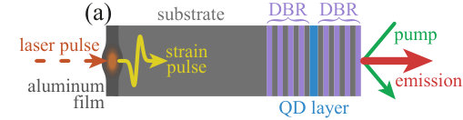 Figure 1
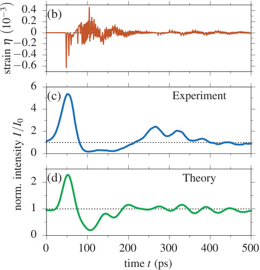 Figure 1
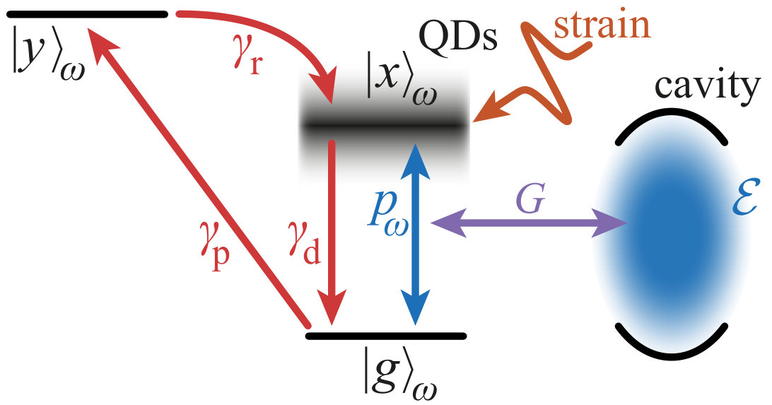 Figure 2
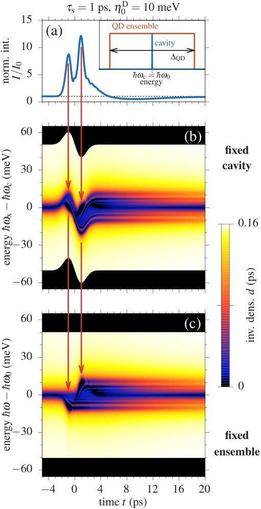 Figure 3
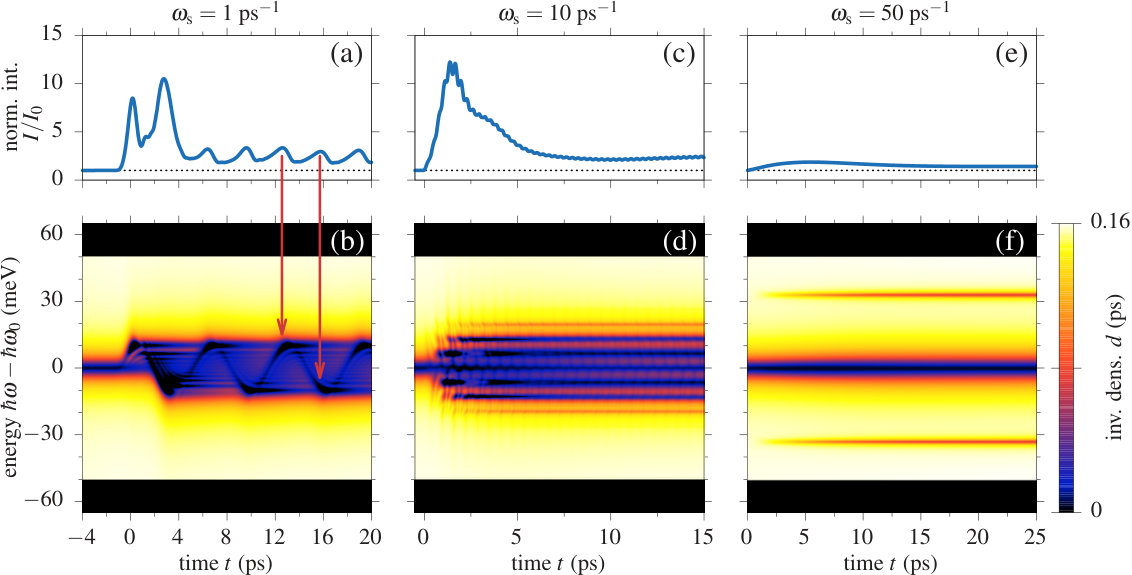 Figure 4
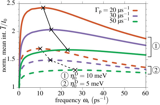 Figure 5
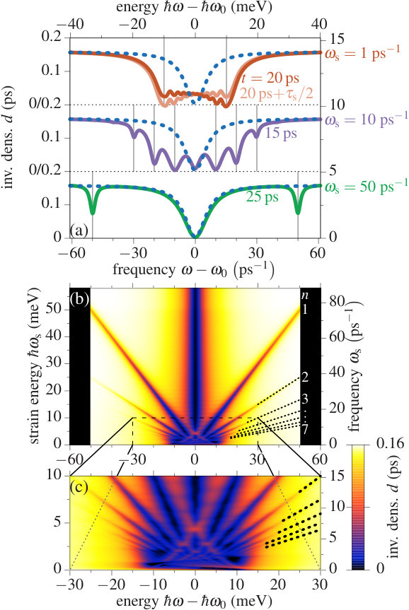 Figure 6
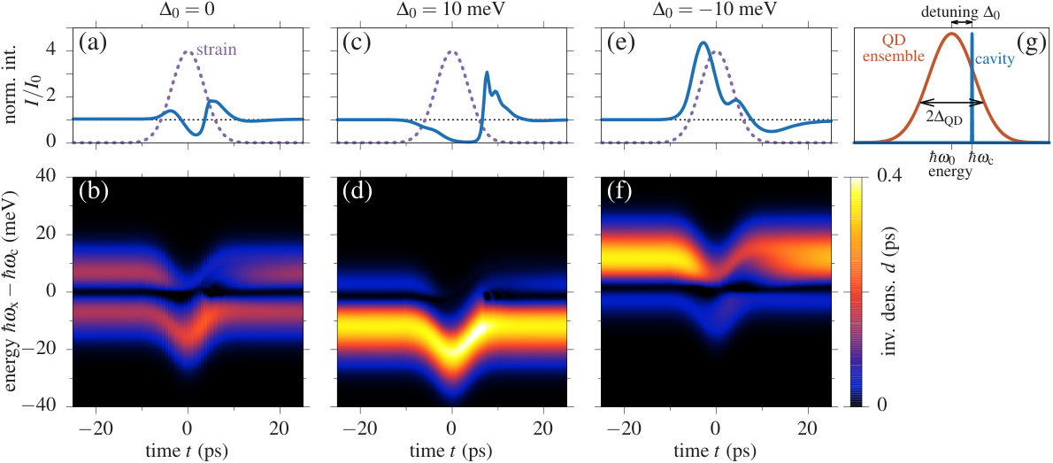 Figure 7
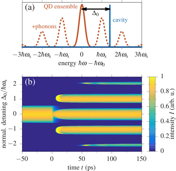 Figure 8
Peer Reviews
No public reviews on file for this paper yet. If you reviewed it on a platform where reviews are public (OpenReview, ICLR, NeurIPS, ICML), you can paste yours below so the community can read it here.
Videos
No videos yet. Explain this paper in a talk, walkthrough, or lecture? Add one.
Systematic study of the influence of coherent phonon wave packets on the lasing properties of a quantum dot ensemble
D. Wigger
Institut für Festkörpertheorie, Universität Münster, 48149 Münster, Germany
T. Czerniuk
Experimentelle Physik 2, Technische Universität Dortmund, 44221 Dortmund, Germany
D. E. Reiter
Institut für Festkörpertheorie, Universität Münster, 48149 Münster, Germany
M. Bayer
Experimentelle Physik 2, Technische Universität Dortmund, 44221 Dortmund, Germany
T. Kuhn
Institut für Festkörpertheorie, Universität Münster, 48149 Münster, Germany
Abstract
Coherent phonons can greatly vary light-matter interaction in semiconductor nanostructures placed inside an optical resonator on a picosecond time scale. For an ensemble of quantum dots (QDs) as active laser medium phonons are able to induce a large enhancement or attenuation of the emission intensity, as has been recently demonstrated. The physics of this coupled phonon-exciton-light system consists of various effects, which in the experiment typically cannot be clearly separated, in particular because due to the complicated sample structure a rather complex strain pulse impinges on the QD ensemble. Here we present a comprehensive theoretical study how the laser emission is affected by phonon pulses of various shapes as well as by ensembles with different spectral distributions of the QDs. This gives insight into the fundamental interaction dynamics of the coupled phonon-exciton-light system, while it allows us to clearly discriminate between two prominent effects: the adiabatic shifting of the ensemble and the shaking effect. This paves the way to a tailored laser emission controlled by phonons.
I Introduction
At the heart of the growing field of phononics lies the active use of lattice vibrations in micro- or nanoscale solid state materials. Many applications, ranging from the excitation of confined phonon modes in optomechanical systems Cleland (2009); Aspelmeyer et al. (2014); Volz et al. (2016) to the control of confined few-level systems by traveling surface acoustic waves Couto et al. (2009); Metcalfe et al. (2010); Gustafsson et al. (2014); Schülein et al. (2015); Golter et al. (2016), prove that phonons have a great potential to drive and control various solid state systems. A key optical application of solid state structures is the semiconductor laser. Here semiconductor quantum dots (QDs) play an increasing role as active laser medium and, in the extreme limit, even a single QD has been shown to give rise to lasing Michler (2003); Strauf and Jahnke (2011); Chow et al. (2014). While carrier-phonon interaction is an important ingredient for energy relaxation, e.g., when bringing carriers from the wetting layer into the laser-active QDs, for the laser process itself the coupling to phonons often does not play a crucial role. Only recently, the two fields – phononics and semiconductor laser physics – have been combined by using traveling coherent phonon wave packets to control the laser output Brüggemann et al. (2012); Czerniuk et al. (2014, 2015). We want to briefly recap these findings: In such an experiment, which is schematically shown in Fig. 1(a), a layer of QDs, surrounded by two distributed Bragg reflectors (DBRs), is used as the active laser medium, which can be pumped optically Brüggemann et al. (2012); Czerniuk et al. (2014) or electrically Czerniuk et al. (2015). By rapidly heating an aluminum film a coherent phonon wave packet is created, which travels through the structure. Due to nonlinear propagation in the material and the transit through the Bragg mirror the strain profile arriving at the QD layer, shown in Fig. 1(b), is rather complex. When the phonons impinge on the QDs the strain shifts the frequency of the optical transition in the QDs. As a result, the laser output can be greatly enhanced, but also quenching can be induced. This is demonstrated in Fig. 1(c), where an example of the measured laser intensity normalized to the stationary state intensity is shown. A detailed interpretation of the coupled phonon-exciton-light system is rather sophisticated because depending on the spectral properties of the QD ensemble and the time scale associated with the phonon dynamics different phenomena contribute to the observed modulation of the laser output.
We here develop and investigate a semiclassical laser model, as depicted in Fig. 2, to describe the dynamics of the coupled system consisting of coherent phonon wave packets, QD excitons and laser light. Our model has already been shown to well reproduce the experimentally observed laser outputs Czerniuk et al. (2017). In this paper we now use the model to gain a deeper understanding of the coupled phonon-exciton-light system by systematically studying different ensemble and strain scenarios. Due to the complex strain pulses present in the experiment, a clear interpretation and in particular a separation between different phenomena is still challenging. Two effects turned out to be important, when controlling the laser output: On the one hand the adiabatic shift of the ensemble, which dynamically changes the number of QDs in resonance with the laser cavity. On the other hand the shaking effect of the ensemble, which rapidly brings initially detuned and therefore highly occupied QD excitons into resonance with the cavity. In this paper, we are going to use this model to systematically study the influence of the phonons on the lasing activity and to discriminate between the phenomena of shifting and shaking. For this purpose, we will use idealized ensemble shapes (e.g., a flat distribution of QD transition energies) and idealized strain pulses (e.g., bipolar or monopolar pulses or monochromatic phonons) which will allow us to separate the shaking effect from the adiabatic shift in an intuitive way.
By providing a thorough understanding of the coupled phonon-exciton-light system, we are not only able to understand the complex laser emission seen in the experiment, but we also lay the foundation to optimize the system, which will then stimulate further studies on phonon control of solid state lasers and pave the way for designing applications.
The paper is structured as follows: In Sec. II the basics of the semiclassical laser model are summarized. The results are given in Sec. III, first for a rectangular QD distribution in part III.1 and second for a Gaussian ensemble in part III.2. In Sec. IV we come back to the experimental results in Fig. 1 and provide a detailed interpretation on the basis of the results for the idealized cases. The paper closes with some concluding remarks in Sec V.
II Theoretical model
To model the QD laser system we employ a semiclassical laser model in the usual dipole, rotating wave and slowly varying amplitude approximation Haken (1970). The QDs are taken to be in the strong confinement limit, such that for the coupling to the laser mode and the coherent phonons they can be reduced to two-level systems consisting of ground state and exciton state with transition frequencies , labelling the individual QD and being the number of QDs in the ensemble. The QD is coupled via the dipole matrix element to the light field, treated as a classical field with positive (negative) frequency component () as well as to the acoustic phonons, described by the phonon creation (annihilation) operators (), denoting the phonon wave vector. The Hamiltonian of the QD ensemble then reads
[TABLE]
and the exciton-phonon coupling matrix element . From the Hamiltonian and Heisenberg’s equation of motion we obtain the equation of motion for the microscopic polarization as well as the occupations and . After truncating the electron-phonon correlation expansion on the mean field level, which is appropriate for the description of the coupling to an external coherent phonon wave packet, we get
[TABLE]
The dominant exciton-phonon coupling in typical InGaAs-based QDs is provided by the deformation potential coupling. For this mechanism the mean field contribution can be written as Krummheuer et al. (2005a)
[TABLE]
with being the expectation value of the lattice displacement at the position of the QD and is the corresponding strain. is the deformation potential of the exciton with () being the deformation potentials of electrons and holes. From Eq. (2) we can therefore conclude that the transition energy of each QD is shifted from the unstrained value to a time-dependent value , the shift being proportional to the strain value at time , according to
[TABLE]
By taking the strain field at the position of the QD we have implicitly assumed that the wavelength of the phonons contributing to the phonon wave packet is much larger than the size of the QDs, such that the strain value does not vary over the size of the QD. Typical values for the deformation potential are in the range of eV Krummheuer et al. (2005b). Together with the strain amplitudes in the experiment [see Fig. 1(a)] energy shifts of a few meV are reached. In the following we will directly treat the product as a strain mediated energy shift. In the current form of the strain control it is a good assumption to treat the phonons as plane waves hitting the QD layer perpendicularly, such that at a given time all QDs in the ensemble experience the same shift. One could also think of phonon wave packets that arrive at a certain angle at the QD layer or that travel in-plane through the QD ensemble, where QDs at different positions would interact with different parts of the strain wave. For the description of such a scenario a spatio-temporal extension of the QD laser model would be needed Hess and Kuhn (1996a, b); Gehrig and Hess (2002); Gehrig et al. (2004).
Because the exciton transition energies in the QD ensemble are closely spaced, we introduce the spectral distribution of the ensemble
[TABLE]
and move to a continuous description labeling the QDs by their transition frequencies, i.e., , , and . The dynamics of the cavity field is driven by the macroscopic polarization of the whole ensemble
[TABLE]
where we have assumed that the variation of the dipole matrix elements over the QD ensemble is negligible. By separating the electric field into the normalized mode function of the microcavity and a time-dependent amplitude according to and introducing the dimensionless cavity field amplitude with we can write
[TABLE]
with the coupling constant
[TABLE]
Here, denotes the cavity frequency, is the vacuum permittivity and we have assumed that the coupling constant has approximately the same value at all QDs of the ensemble, which is reasonable since all QDs are in a thin layer in the center of the cavity.
To simulate the pumping process we include the occupation of an additional level , which can be thought of as wetting layer state and is phenomenologically coupled to the other levels via constant rates. With this we finally arrive at the following closed set of equations Haken (1970):
[TABLE]
where is the detuning between the cavity mode and the considered exciton transition. Note that the equations are given in a frame which rotates with the frequency of the cavity mode. To simulate the vacuum fluctuations and start the lasing process we add a white noise source to the field amplitude in every time step. The rates in the equations include the pump rate from to , the relaxation rate from to and the spontaneous decay rate from to as shown in Fig. 2. Additionally describes the cavity loss rate and a pure dephasing rate, which only acts on the polarization . Following the results in Ref. Czerniuk et al. (2017) we choose the same parameters for the laser system, i.e., ps*-1*, ps*-1*, ps*-1*, ps*-1*, and ps*-1*. Already in Ref. Czerniuk et al. (2017) it was shown that the strongest laser response on the strain field happens for pump rates that are slightly above the threshold pump rate, which for our system parameters is approximately the spontaneous decay rate . Thus we define a shifted pump rate as
[TABLE]
III Results
The main goal for the paper is to separate various effects which contribute to the modulation of the laser output, in particular the shaking and the adiabatic shift. To eliminate the latter one, we first consider a QD ensemble in which the number of dots in resonance with the cavity mode remains constant when the exciton energy varies. The Gaussian ensemble, will be discussed in Sec. III.2.
The central quantity to illustrate the dynamics of the QD ensemble is the inversion density
[TABLE]
which indicates how many QDs with a given transition frequency are in the excited state. It further reflects the spectral shape of the ensemble.
III.1 Ensemble with rectangular QD distribution
To analyze the shaking effect we choose an idealized ensemble shape being rectangular with the spectral QD density given by
[TABLE]
where is the total number of QDs and is the width around the center of the ensemble. By this choice the number of QDs in resonance with the laser cavity is always the same, as long as the cavity resonance stays in the range of the ensemble. A schematic picture of the ensemble is shown in the inset in Fig. 3(a). The cavity resonance is supposed to be initially in the center of the ensemble. Since the pumping is taken to be the same for the whole ensemble, an energetic shift of the ensemble will bring highly occupied QD excitons into resonance with the cavity and therefore influence the output of the laser. This process is called shaking of the
III.1.1 Single strain pulse
We start our investigation with a single bipolar strain pulse leading to the energy shift
[TABLE]
where the pulse is centred around and has a width of between minimum and maximum. In the following, the maximum amplitude of the energetic shift will for brevity be referred to as strain amplitude, but note that this always represents the product . The negative sign in Eq. (13) reflects the negative sign of the deformation potential and has been introduced such that a positive strain corresponds also to a positive value of . The strain dynamics in Eq.(13) corresponds to a Gaussian phonon wave packet in the lattice displacement, which is for example generated initially in the experiment Scherbakov et al. (2007) or by an ultrafast optical excitation of a single QD Wigger et al. (2013).
Figure 3 summarizes the response of the QD laser system on the interaction with a strain pulse given by Eq.(13) with a duration of ps and a strain amplitude of meV, the width of the QD ensemble is meV. The strain pulse arrives, when the laser has reached its stationary state. We choose the pump rate to µs*-1*. The laser intensity normalized to the intensity without any strain is plotted in Fig. 3(a) as a function of time . The laser output is dominated by two enhancement peaks that reach values of about . The maxima are at the positions of the extrema of the strain pulse, marked by red arrows. After the pulse the intensity shows a period of attenuation around ps and eventually goes back to 1.
To get a better insight into the origin of the variation of the laser output Fig. 3(b) and (c) show the inversion density as a function of time and exciton energy . Because in the equation of motion for the microscopic polarization [Eq. (9)] only the detuning between the cavity mode and the considered QD energy enters, it is not important for the simulation if the QD transition energies are shifted by the strain according to Eq. (4) or if all QD transitions stay at the same energies and the cavity resonance is shifted by the same amount but in the opposite energetic direction. Thus it is possible to present the dynamics of the inversion density of the QD ensemble either with a fixed cavity resonance energy and a strain affected QD ensemble (i.e., as a function of ) or with a fixed ensemble distribution () and a cavity resonance that is shifted by the strain dynamics. The former is realized in Fig. 3(b) and the latter in (c). Both representations are shown here because in either case different aspects of the inversion dynamics can be explained more easily. Before the strain pulse, i.e., at ps both inversion density representations look the same. The region between and 50 meV depicts the spectrum of the QD ensemble, for larger energies there are no QDs which results in a vanishing density (black). At the edges of the ensemble the QDs are highly occupied, which is seen by the bright color, but in the center, at the position of the cavity mode, an energy range with reduced inversion densities appears. This depression of the exciton occupation represents the QDs that contribute to the laser process and is called spectral hole. During the interaction with the strain pulse, i.e., for ps, the actual influence of the strain can be seen. Let us first focus on the representation in (b). The energetic position of the ensemble is shifted proportional to the strain amplitude, therefore the complete colored area shifts to larger energies, reaches a maximum shift of meV at ps (left red arrow). It is then shifted toward smaller energies, reaching again the maximum shift at 1 ps (right red arrow) and goes back to its initial position. During the whole process the cavity resonance stays at . In contrast, the spectral hole does not stay at the energy of the cavity, it rather follows the strain shift of the ensemble toward positive energies. While this happens the shape of the spectral hole is strongly modified. After the strain pulse at ps the final spectral hole consists of multiple minima distributed symmetrically around the cavity at 0 meV. For increasing times the outer inversion minima decay and only the original spectral hole remains when the laser comes back to its steady state.
We now come back to the laser output in (a) and directly compare the enhancement and attenuation features with the inversion density. The red arrows mark both the maxima of the laser intensity and the extrema of the strain shift. At the arrowheads two dark spots appear in (b), which represent very small or even negative values of . Note that due to clarity the color scale in Fig. 3(b) and (c) starts at , although negative values may appear when stimulated emission de-occupies a QD exciton. The origin of these strong spectral holes can best be explained in the picture of a fixed ensemble and a strain shifted cavity resonance in (c). The fact that the edges of the colored area are fixed shows that the QD energies are unaffected by the strain. Due to the strain shift of the cavity resonance it first moves to smaller energies and reaches meV at ps, which is marked by the left red arrow. We see that at this time the strong deepening of the spectral hole happens. The reason is, that the cavity moves toward highly occupied QDs faster than they can fully react on the presence of the cavity mode. When the cavity shift reaches its maximum at ps, the shift is sufficiently slow for the QDs that are in resonance with the cavity during that time window to emit stimulatedly into the laser mode. Due to this switch-on process of QDs that were previously not in resonance with the laser mode, the output increases drastically resulting in the first peak in (a). The same happens for the second turning point of the strain shift at ps. After the strain has shifted the cavity out of resonance again the QDs in these two strong spectral holes are significantly detuned from the laser mode and can not contribute to the laser output any more. The re-occupation of the dots appears as decay of the spectral holes. The last feature of the laser intensity in (a) is the attenuation between and 16 ps. After the strain pulse, the cavity resonance is again at the center of the ensemble and the QDs in the region of the additional outer spectral holes do not contribute to the laser process any longer. This means that only the QDs within the spectral hole at ps, i.e., before the strain pulse, are important for the intensity. A close look at the shape of the central spectral hole reveals that it is less deep than before the strain pulse. During the pulse the QD excitons within the spectral hole were detuned from the cavity resonance and are therefore higher occupied directly after the pulse. They need a while to reach the stationary laser state, which has smaller inversions, i.e., a deeper spectral hole. This also results in the reduced intensity. The original stationary laser state recovers completely at ps.
As a side remark, we note that for strain pulses that are significantly longer in time ( ps) the spectral hole can adiabatically follow the shift of the ensemble, such that always the same amount of QDs takes part in the laser process and the intensity stays constant (not shown).
III.1.2 Harmonic modulation
We have seen that a shift of the QD ensemble on the picosecond time scale brings the laser system out of equilibrium and results in variations of the output intensity on the order of tenfold enhancements. In the second example we tackle the question, under which conditions a laser system driven by a harmonic strain perturbation reaches a new stationary state.
Besides the fundamental interest, such a study is well connected to recent research. Monochromatic coherent phonons can be optically created in semiconductor superlattices. A recent experiment demonstrates narrow band phonon generation with frequencies of more than 2 THz Huynh et al. (2008); Jiang et al. (2016), which is comparable to the values studied in the following. To make maximum use of these vibrations, one can tailor a phononic cavity for the desired phonon frequency and embed it into the optical resonator – in this way the generated phonons become confined in the same place as the active medium Trigo et al. (2002). In passive optomechanical resonators the localization of phonons and photons results in an enhanced coupling strength Fainstein et al. (2013), while in a laser device the resonant strain field leads to a harmonic modulation of the lasing emission Czerniuk et al. (2014). We model the harmonic strain field by:
[TABLE]
i.e., the harmonic strain oscillation is smoothly switched on between and , where is the period of the strain frequency . The laser has reached its stationary output long before the strain oscillation is switched on.
In Fig. 4 three different strain frequencies are shown for a pump rate of µs*-1*. In the left column [(a), (b)] we have ps*-1*, in the middle [(c), (d)] ps*-1* and on the right [(e), (f)] ps*-1*. The upper row presents the normalized laser intensity as a function of time and the bottom row the inversion density for a fixed ensemble as a function of time and exciton energy . Note that in this representation the energy of the cavity resonance is shifted by the strain.
We start the discussion of the harmonically driven laser system with ps -1 in (a) and (b). In the normalized laser output in (a) two features can be distinguished: On the one hand two strong enhancement peaks between ps and 4 ps and on the other hand an oscillation around for ps. The double peak structure at the beginning looks very much like the dynamics in Fig. 3(a) and also the behavior of the inversion density in (b) shows the above explained appearance of additional spectral holes at higher energies. Thus we conclude that the features are due to the switch on of the strain oscillation. The new feature is the oscillatory part for ps, which has a period of half the strain period ps. The two red arrows mark maxima of the intensity, which directly correspond to extrema of the strain oscillation. The movement of the cavity resonance can be seen in (b) as oscillating dark line around 0 meV. At every antinode of the strain shift the cavity moves slower and the QDs have time to contribute to the laser process more efficiently, which leads to the maxima in the intensity. Around the nodes the QD emission can not follow properly and the intensity drops again. In contrast to the pulsed excitation in Fig. 3(a) the intensity does not go back to . This can easily be understood from the dynamics of the outer spectral holes in Fig. 4(b). Like in the pulsed case they decay after the cavity has moved out of resonance with the respective QDs but gets back into resonance before the excitons are fully re-occupied. Overall we find a broadening of the spectral hole for all times after the strain field is switched on. This broadening spreads over the full energy range that is covered by the strain shift of the cavity resonance (or of the ensemble).
The situation shows some decisive differences when increasing the strain frequency to ps*-1* in Fig. 4(c) and (d). The normalized intensity in (c) is still dominated by a pronounced maximum lasting from to about 7 ps, which arises from the switch-on process of the strain oscillation. At 15 ps the output has almost reached a stationary value of about . Still the whole curve is covered with an oscillation with half the strain period ps, but with very small amplitudes compared to the previous example. Also a very different picture is found for the inversion density in (d). The oscillation of the cavity resonance in form of a dominating spectral hole is no longer resolved. Within the first 5 ps multiple clearly separated spectral holes appear symmetrically around . Apparently now a wide range of exciton energies contribute to the laser process and lead to the significantly increased, almost constant, laser intensity. A surprising feature is the appearance of spectral holes at energies larger than the strain shift of meV. The four outer most lines in the plot are clearly above meV. We will come back to this point in more detail below.
The appearance of spectral holes at large energies becomes even more striking when increasing the strain frequency further to ps*-1* in Fig. 4(f). After the strain field is switched on the inversion density reaches a stationary state after approximately 25 ps. Three well separated spectral holes show up. While the one in the middle does not change significantly from the unstrained case two additional ones appear at approximately meV. For the laser intensity in (e) this enlarged number of QDs contributing to the laser output leads to a slight increase. Obviously the final intensity enhancement is smaller than in the case in (c). Thus it can be expected that the strain frequency follows some sort of resonance condition.
Before coming back to the shape of the spectral hole under the strain influence, we want to embark on the dependence of the enhancement on the strain frequency. Figure 5 shows the normalized mean final intensity as a function of the strain frequency for different strain amplitudes and pump rates as listed in the picture. Every curve shows a more or less pronounced maximum supporting the prediction, that the strain induced enhancement works most efficiently for a characteristic frequency. For very small strain frequencies the laser system can follow adiabatically and for very fast oscillations the laser system is too inert and the response reduces again. We also see that for higher strain amplitudes the enhancement factors increase. This is intuitive because the strain-induced shift reaches a larger amount of QDs if the amplitude of the shift is larger. With a close look at the positions of the maxima (marked by the crosses in Fig. 5) we find that the peak frequency shifts to larger values for increasing pump rates. Thus the characteristic frequency of the laser system becomes larger for growing pump rates. This growth of the characteristic frequency can also be connected to the relaxation oscillations during the switch-on of the laser. An example of the relaxation oscillations in our system can be seen in Fig. 7(c). It is well known that also the frequency of the relaxation oscillations grows with increasing pump power Bimberg et al. (2000).
The next focus is on the shape of the spectral hole and its dependence on the strain frequency, which was already mentioned when discussing Fig. 4. We have found that multiple depressions appear in the inversion density. While for small strain frequencies these are restricted to the strain shift amplitude, for increasing frequencies the additional spectral holes also appeared at larger energies. To get a more quantitative picture Fig. 6(a) shows the inversion density at the end of the time windows shown in Fig. 4(b), (d) and (f) from top to bottom, respectively. As a reference the spectral hole without any strain is always plotted as dotted blue line. Note that the bottom x-axis shows the exciton frequency , while the top one gives the energy . For the case of ps*-1* (top, dark red) the spectral hole is very broad with a rather flat base line, which has a slight negative tilt. That the slope of the tilt oscillates with the strain frequency is confirmed by the bright red curve, which shows the same inversion density but half a strain period later. The complete hole spreads over the energy range, which is covered by the strain shift ( meV) as can be seen from the two vertical lines. The middle panel presents the ps*-1*-case. Here we want to focus on the frequency axis at the bottom. As marked by the vertical lines, the well separated minima in the inversion density are exactly at multiples of the strain frequency, i.e., at , and ps*-1*. This is further confirmed in the bottom panel for ps*-1*. Here the additional spectral holes lie at ps*-1*. The second one would appear at ps*-1*, which is already outside of the ensemble.
We can conclude that additional spectral holes appear at energies with
[TABLE]
i.e., at higher harmonics of the strain frequency.
To develop a complete picture of the strain frequency dependence of the spectral hole Fig. 6(b) and (c) show the inversion density of the QD ensemble at a fixed time long after the switch-on process of the strain field as a function of the exciton energy and the strain energy according to its frequency . Panel (c) is a zoom-in on the dashed area in (b). Focussing first on the large energy range in (b) we see that the central spectral hole at the initial position of the cavity is almost unperturbed by the strain field. For large strain energies the additional spectral holes show up as diagonal lines that decay for increasing energies. The dotted black lines follow Eq.(18) together with the number of the higher harmonics given on the right. Within the Floquet theory it is shown that a harmonically driven two level system with the energy splitting has multiple additional so called Floquet states at energies , where is the driving frequency. Therefore QDs that are detuned from the cavity mode by multiples of the strain frequency gain new transitions that are in resonance with the cavity. By this they can contribute to the laser process. A more intuitive interpretation of the addition transitions is as follows: Because the QD ensemble is interacting with a phonon system with a discrete spectrum, single or multiple absorptions and emissions of phonons are possible to overcome the detuning to the cavity mode. Accordingly, the outer spectral holes arise from excitons, which contribute to the laser process via phonon assisted transitions. Focussing on the region of small energies in (c) we find a transition area from the adiabatic situation ( meV), where the spectral hole at the position of the cavity mode can immediately follow the shift of the ensemble, toward the formation of the additional higher harmonic spectral holes for strain energies meV. Below this energy the widening of the spectral hole is restricted to the range of energies that is covered by the strain amplitude , i.e., meV. Below meV also the central spectral hole is not well developed and vanishes within the whole broadening.
III.2 Gaussian ensemble
In the second example, we now want to focus on the adiabatic shift. For this purpose we choose a QD ensemble shape with a Gaussian distribution given by
[TABLE]
which is the same as in Ref. Czerniuk et al. (2017). Any energetic shift of the ensemble leads to a variation of the number of QDs in resonance with the cavity mode, therefore the adiabatic shift of the ensemble does inevitable play an important role. On the other hand the shaking effect cannot be suppressed by a specific choice of the ensemble and will always contribute. A schematic picture of the ensemble is given in Fig. 7(g), which also shows the initial detuning
[TABLE]
between the cavity mode and the ensemble center. The total number of QDs is again .
III.2.1 Single strain pulse
As a starting point we choose a monopolar strain pulse to interact with the system. Such pulses have also an experimental counterpart, namely acoustic solitons, which develop during the nonlinear propagation of the phonons. They are of special interest, since they combine high frequency phonons with a very small spatial extension of only a few nanometers. The dynamics is given by a single Gaussian of the form
[TABLE]
The amplitude of the strain shift is and the width is given by . This strain dynamics is a good approximation for soliton pulses, which develop during the nonlinear propagation of acoustic pulses Van Capel et al. (2015) [cf. Fig. 1(a)]. This choice of the strain pulse is even simpler than the bipolar pulse in Eq. (13), in order to demonstrate the effect of the adiabatic ensemble shift more transparently. Figure 8 shows the results for an ensemble width of meV, a pump rate of ps*-1*, a strain amplitude of meV and a pulse duration of ps.
We start the discussion with the special case of vanishing initial detuning . Due to the symmetry of the system the reaction on the strain pulse does not depend on the sign of the shift. The results for the normalized laser intensity are shown in Fig. 7(a) (solid blue) together with the strain pulse (dotted violet). We see that the laser output is first increased, then decreased and increased another time during the time of the strain pulse. We directly compare these dynamics with the behavior of the inversion density in (b), which is here shown for a fixed cavity resonance, i.e., against the energy . Thus in the figure the ensemble is shifted by the strain field. Before the strain pulse we clearly see the spectral hole in the center of the Gaussian QD distribution, during the pulse the ensemble shifts to smaller energies and therefore out of resonance with the cavity. Without the shaking effect, we would expect a drop of the laser intensity, because the number of QDs in resonance with the laser mode is reduced during the first half of the strain pulse. However, we contrary first observe an increase of the intensity in (a), which proves that the shaking effect outweighs the adiabatic response due to the reduced number of resonant QDs. Likewise the attenuation of the output can be understood because it happens at the maximum of the strain shift, which happens much slower and the adiabatic shift becomes more important. During the second half of the strain pulse the ensemble is brought back into resonance with the cavity, such that the shaking effect and the adiabatic shift work in the same direction and result in a slightly stronger enhancement in (a). As can be seen in (b) around the inversion density increases while the ensemble is out of resonance with the cavity. When these re-occupied dots get back into the cavity mode they can emit and contribute to the laser process.
In the other two examples the initial detuning is chosen in the same order as the strain amplitude. In (c) and (d) the initial detuning is meV, but the strain shifts the ensemble further away from cavity. For the laser intensity in (c) this means a complete quenching at . During the second half of the strain pulse the laser is switched on again exhibiting the characteristic relaxation oscillations before reaching its original intensity. In the inversion density in (d) we see that the spectral hole is now at the edge of the ensemble. During the strain pulse the ensemble shifts to even smaller energies and the spectral hole in the cavity resonance vanishes, leaving an almost completely occupied Gaussian ensemble. When the ensemble moves back into resonance with the cavity also the dynamics of the spectral hole reveal the relaxation oscillations. To conclude, the strain leads to a switch-off of the laser due to the adiabatic reduction of resonant QDs. The pronounced enhancement of the output happens due to the switch-on process of the laser and is part of the characteristic relaxation oscillations.
In Fig. 7(e) and (f) the situation is inverted, the initial detuning is chosen to meV and the strain pulse shifts ensemble and cavity into resonance at its maximum. In the intensity in (e) this leads to a strong enhancement peak. At the end of the pulse around ps we also find a significant reduction of the output. Looking at the inversion density in (f) we see that initially the main part of the ensemble is on the other side of the cavity. The strain pulse then reduces the detuning. It is clearly visible that most of the QDs become de-occupied around . When this large number of QDs emits stimulatedly into the cavity mode, the large enhancement in (e) is observed. Also while the ensemble is shifted back to the original detuning situation at ps, the laser field is still enhanced. On the other hand due to the previous stimulated emissions there is a reduced number of occupied excitons, which are not capable of feeding the laser process. Therefore the intensity drops below , while enough dots recover their occupation. The system reaches its initial stationary value after ps.
III.2.2 Harmonic modulation
In this part we come back to the switched on harmonic strain oscillation from Eq.(III.1.2) and apply it to a Gaussian ensemble. We choose a small ensemble width of meV, a strain frequency of ps*-1* and a strain amplitude of meV. Note that these parameters were chosen to optimize the visibility of the effect. Figure 8(a) shows a schematic picture of the QD ensemble (solid orange) together with the cavity mode (blue). Following the arguments of the Floquet theory in Sec. III.1 the interaction with the single frequency phonons of the strain field will lead to additional satellite replicas of the ensemble shifted by multiples of the strain energy , which are indicated by the dotted orange curve. This effect has been seen in photoluminescence spectra of single QDs that were driven by surface acoustic waves Metcalfe et al. (2010).
In Fig. 8(b) we see the laser intensity as a function of time and detuning normalized with respect to the strain energy . Before the switch-on of the strain oscillation, i.e., for ps, we find an approximately Gaussian profile of the emission intensity, which directly resembles the ensemble shape because the laser intensity increases with the number of resonant QDs. When the strain field is switched on additional yellow lines appear at multiples of the strain energy. This shows that the laser system also works in a completely phonon assisted situation. A close look at the intensity amplitudes of the assisted lines shows that they are less strong than the central resonant one. When the strain field is switched on at also the central line is significantly narrowed due to the interaction with the phonons, but recovers almost completely after 150 ps. The lines at appear later, because it takes more time for the system to start and reach the final output. Here it is more clearly visible that their intensity is less strong, reaching only half the resonant amplitude.
IV Comparison to experiment
With our newly gained knowledge we close the discussion by shortly revisiting the experimental results in Fig. 1. Let us first comment on the complex strain pulse, which is obtained in the experiment. Its dynamics arises from the propagation of the phonons through the sample before reaching the active medium. The injection of the acoustic pulse happens via an intense picosecond laser pulse that rapidly heats an aluminum film as shown on the left side of Fig. 1(a). The heating is associated with an expansion of the film, which launches a phonon wave packet with an approximately Gaussian lattice displacement into the substrate material. This lattice displacement corresponds to a bipolar strain pulse of about 20 ps. Due to the large strain amplitudes on the order of nonlinear effects have to be taken into account in the phonon propagation through the substrate Scherbakov et al. (2007); Van Capel et al. (2015). During this propagation solitons form and the strain pulse gets stretched over a few tens of picoseconds. Before reaching the QD layer of the sample the strain pulse is additionally modified by passing through the bottom DBR [left one in Fig. 1(a)]. Multiple transmission and reflection processes in the DBR then lead to the final dynamics in Fig. 1(b) that lasts several hundreds of picoseconds.
In the laser output [Fig. 1(c)] we find first a strong enhancement peak followed by 100 ps of almost complete quenching. After 200 ps the output is dominated by a harmonic oscillation, reproduced well by the simulation [Fig. 1(d)]. In the presented example the cavity mode is positively detuned from the QD ensemble, such that negative strain values reduce the detuning and positive ones increase it. Due to our previous analysis we are now able to attribute these variations to the two effects: Through the first negative solitonic strain pulses both – shaking and shifting – lead to an increase of the laser output as it was found in Fig. 7(e). The following attenuation then has two reasons. On the one hand many QDs were de-occupied during the first intensity peak and the initial intensity cannot be preserved any longer. On the other hand the mean strain value is positive, which reduced the laser output naturally through the adiabatic shift. The harmonic oscillation in the last part in Fig. 1(b) arises from the adiabatic shift due to the slow harmonic oscillation of the strain field.
V Conclusion
In summary we have presented a systematic study of the QD laser emission properties driven by coherent phonons. By choosing a rectangular ensemble the adiabatic shift of the ensemble could be suppressed and the shaking effect was analyzed separately. We have shown that the intensity enhancement depends strongly on the time scale of the phonon field. For harmonic strain oscillations phonon assisted transitions contribute to the laser output. For a realistic Gaussian ensemble both effects take part in the process. We have found that depending on the initial detuning, the intensity could either be significantly enhanced or switched-off on an ultra fast time scale.
The detailed study of the different effects allowed us to obtain a deep understanding of the details of the measured intensity modulations. With this, it will be possible to tailor the nanostructure as well as the phonon pulses to reach a desired control of the laser output, may it be a long lasting amplification or a brief enhancement with a strong amplitude. Hence, our work paves the way for further research both on the theoretical side, e.g. for further optimization, and on the experimental side, e.g. to fabricate and measure different structures and phonon pulses.
The demonstrated control of light-matter interaction by acoustic waves may be extended also into the quantum regime, for example for the deterministic generation of single or entangled photons from a quantum dot in an optical microresonator. This can be achieved by shifting the exciton transition dynamically to the optical cavity mode so that a single photon is emitted in resonance condition. Similarly the two transitions in the bixeciton radiative decade maybe sequentially shifted into cavity resonance. Thereby not only true exciton-photon control may be obtained but also the temporal jittering of the photon emission times may be reduced.
VI Acknowledgements
The Dortmund team acknowledges the financial support by the Collaborative Research Center TRR 142. We are grateful for fruitful discussions with Andrey V. Akimov.
The reference list from the paper itself. Each links out to its DOI / PubMed record.
- 1Cleland (2009) A. Cleland, “Optomechanics: Photons refrigerating phonons,” Nature Phys. 5 , 458–460 (2009).
- 2Aspelmeyer et al. (2014) M. Aspelmeyer, T. J. Kippenberg, and F. Marquardt, “Cavity optomechanics,” Rev. Mod. Phys. 86 , 1391 (2014).
- 3Volz et al. (2016) S. Volz, J. Ordonez-Miranda, A. Shchepetov, M. Prunnila, J. Ahopelto, T. Pezeril, G. Vaudel, V. Gusev, P. Ruello, E. M. Weig, M. Schubert, M. Hettich, M. Grossman, T. Dekorsy, F. Alzina, B. Graczykowski, E. Chavez-Angel, J. S. Reparaz, M. R. Wagner, C. M. Sotomayor-Torres, S. Xiong, S. Neogi, and D. Donadio, “Nanophononics: state of the art and perspectives,” Eur. Phys. J. B 89 , 1 (2016).
- 4Couto et al. (2009) O. D. D. Couto, S. Lazić, F. Iikawa, J. A. H. Stotz, U. Jahn, R. Hey, and P. V. Santos, “Photon anti-bunching in acoustically pumped quantum dots,” Nature Photon. 3 , 645–648 (2009).
- 5Metcalfe et al. (2010) M. Metcalfe, S. M. Carr, A. Muller, G. S. Solomon, and J. Lawall, “Resolved sideband emission of In As/Ga As quantum dots strained by surface acoustic waves,” Phys. Rev. Lett. 105 , 037401 (2010).
- 6Gustafsson et al. (2014) M. V. Gustafsson, T. Aref, A. F. Kockum, M. K. Ekström, G. Johansson, and P. Delsing, “Propagating phonons coupled to an artificial atom,” Science 346 , 207–211 (2014).
- 7Schülein et al. (2015) F. J. R. Schülein, E. Zallo, P. Atkinson, O. G. Schmidt, R. Trotta, A. Rastelli, A. Wixforth, and H. J. Krenner, “Fourier synthesis of radiofrequency nanomechanical pulses with different shapes,” Nature Nanotech. 10 , 512 (2015).
- 8Golter et al. (2016) D. A. Golter, T. Oo, M. Amezcua, I. Lekavicius, K. A. Stewart, and H. Wang, “Coupling a surface acoustic wave to an electron spin in diamond via a dark state,” Phys. Rev. X 6 , 041060 (2016).