
TL;DR
This paper introduces the concept of control capacity, a fundamental limit on how quickly a controller can reduce uncertainty in a system, providing a new way to analyze stabilizability in control systems using information-theoretic principles.
Contribution
It defines control capacity for scalar systems, offers a computable characterization, and connects control stabilizability with information capacity, extending classic results to arbitrary moments of stability.
Findings
Control capacity determines stabilizability of scalar systems.
For second-moment stability, recovers classic uncertainty threshold.
Framework parallels Shannon capacity, enabling computation of side-information value.
Abstract
Feedback control actively dissipates uncertainty from a dynamical system by means of actuation. We develop a notion of "control capacity" that gives a fundamental limit (in bits) on the rate at which a controller can dissipate the uncertainty from a system, i.e. stabilize to a known fixed point. We give a computable single-letter characterization of control capacity for memoryless stationary scalar multiplicative actuation channels. Control capacity allows us to answer questions of stabilizability for scalar linear systems: a system with actuation uncertainty is stabilizable if and only if the control capacity is larger than the log of the unstable open-loop eigenvalue. For second-moment senses of stability, we recover the classic uncertainty threshold principle result. However, our definition of control capacity can quantify the stabilizability limits for any moment of stability. Our…
Click any figure to enlarge with its caption.
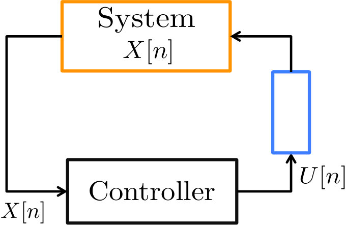 Figure 1
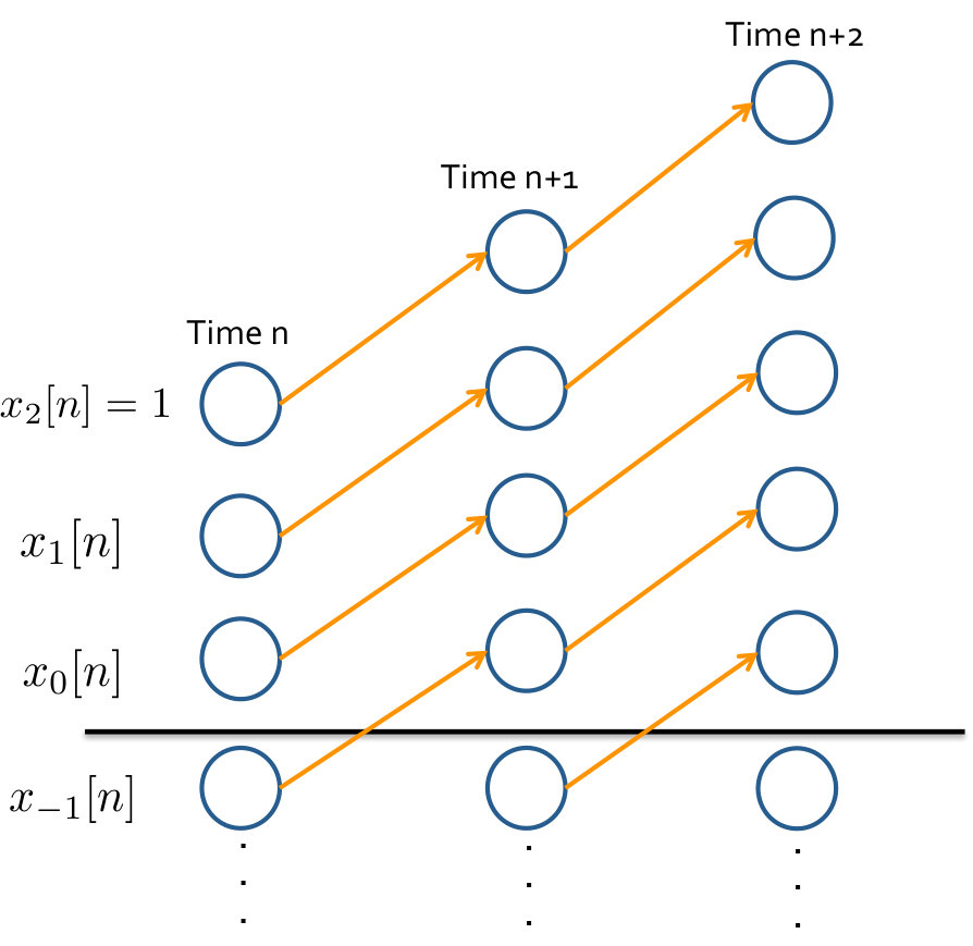 Figure 2
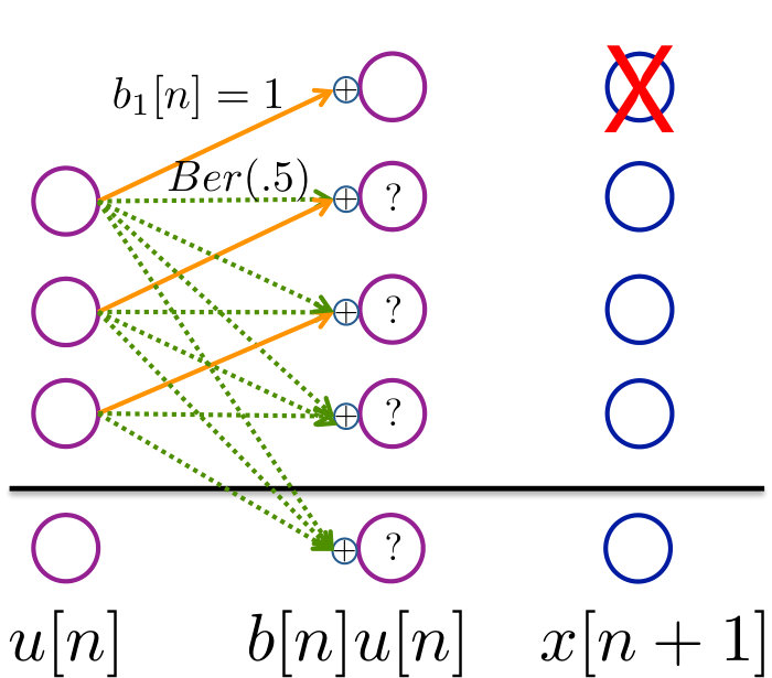 Figure 3
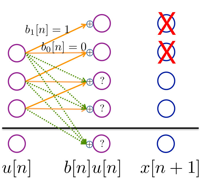 Figure 4
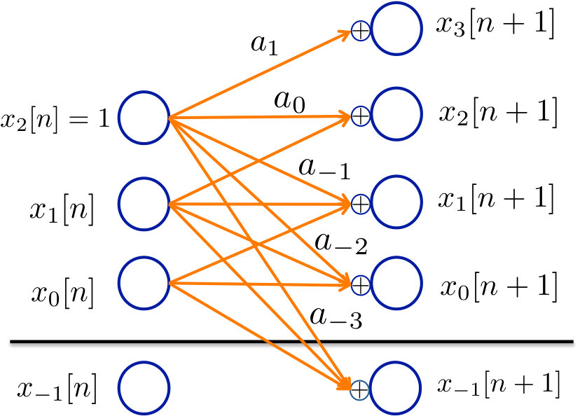 Figure 5
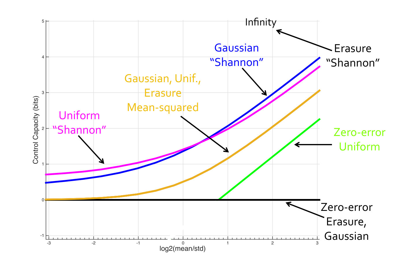 Figure 6
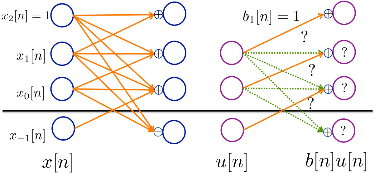 Figure 7
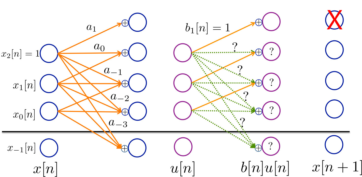 Figure 8
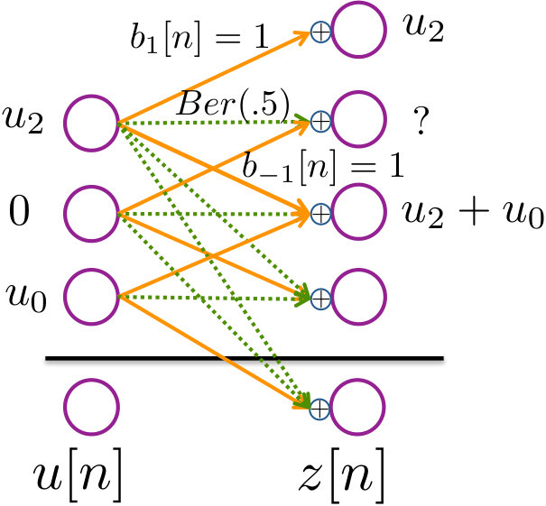 Figure 9
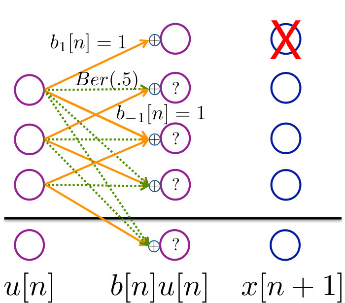 Figure 10
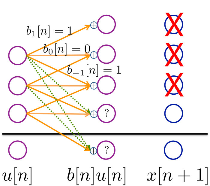 Figure 11
 Figure 12
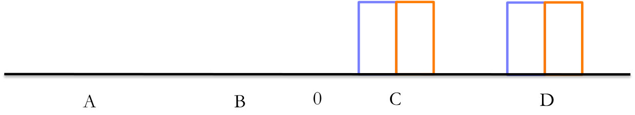 Figure 13
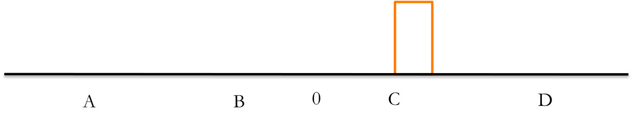 Figure 14
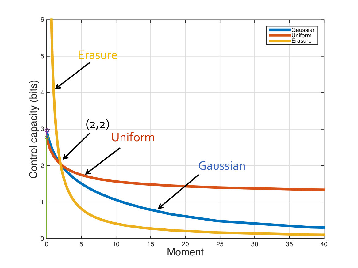 Figure 15
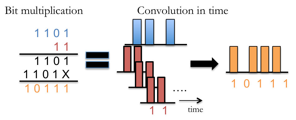 Figure 16
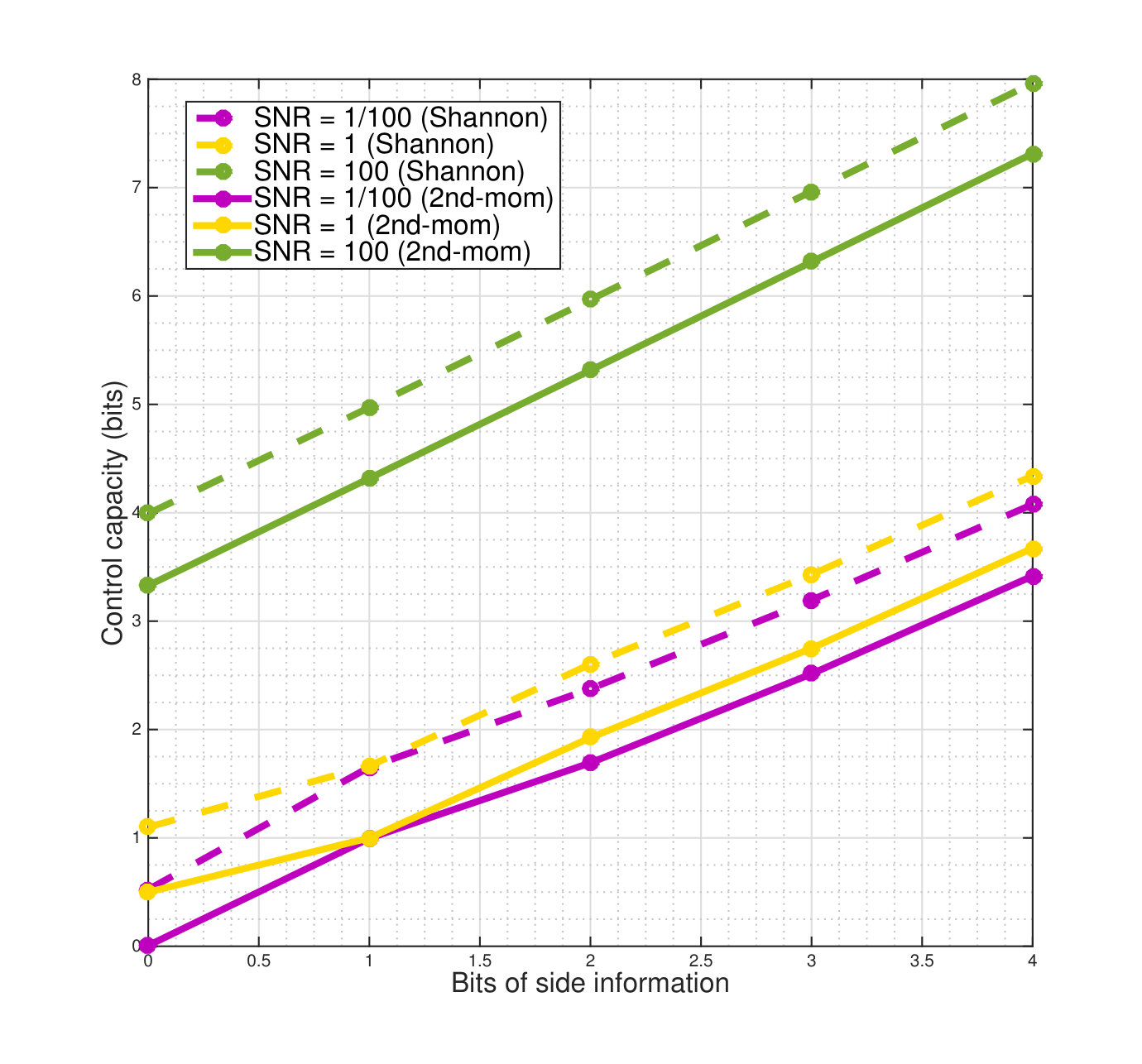 Figure 17
Peer Reviews
No public reviews on file for this paper yet. If you reviewed it on a platform where reviews are public (OpenReview, ICLR, NeurIPS, ICML), you can paste yours below so the community can read it here.
Videos
No videos yet. Explain this paper in a talk, walkthrough, or lecture? Add one.
Taxonomy
TopicsStability and Control of Uncertain Systems · Gene Regulatory Network Analysis · Formal Methods in Verification
Control Capacity
Gireeja Ranade12 and Anant Sahai2
[email protected], [email protected] This paper was presented in part at ISIT 2015 [1] and at ICC 2016 [2]. 1Microsoft Research, Redmond
2Electrical Engineering and Computer Sciences, University of California, Berkeley
Abstract
Feedback control actively dissipates uncertainty from a dynamical system by means of actuation. We develop a notion of “control capacity” that gives a fundamental limit (in bits) on the rate at which a controller can dissipate the uncertainty from a system, i.e. stabilize to a known fixed point. We give a computable single-letter characterization of control capacity for memoryless stationary scalar multiplicative actuation channels. Control capacity allows us to answer questions of stabilizability for scalar linear systems: a system with actuation uncertainty is stabilizable if and only if the control capacity is larger than the log of the unstable open-loop eigenvalue.
For second-moment senses of stability, we recover the classic uncertainty threshold principle result. However, our definition of control capacity can quantify the stabilizability limits for any moment of stability. Our formulation parallels the notion of Shannon’s communication capacity, and thus yields both a strong converse and a way to compute the value of side-information in control. The results in our paper are motivated by bit-level models for control that build on the deterministic models that are widely used to understand information flows in wireless network information theory.
1 Introduction
Shannon’s notion of communication capacity has been instrumental in developing communication strategies over information bottlenecks [3]. This powerful idea provides engineers with a language to discuss the performance of a wide-range of systems going from a single point-to-point link to complex networks.
Just like communication systems, control systems also face many different performance bottlenecks. Some of these are explicitly informational in nature, such as rate-limited channels in networked control systems. Other performance bottlenecks come from the fact that parameters of the system might be uncertain or unpredictable. Model parameters (e.g. mass, moment-of-inertia) must be estimated from data. Other parameters (e.g. linearization constants) might be changing with time; algorithms such as iterated-LQR control require re-linearizing the system at each step.
The impact of of model uncertainty has been investigated by robust control, and robust control provides worst-case bounds on the controllability of a system when only partial information about system parameters is available (e.g. [4, 5]). Many works have also investigated how side-information regarding uncertain parameters can improve the performance of control systems, and this work is discussed later in the introduction. We build on these ideas and are motivated by Witsenhausen’s comments in [6], where he points out the need for a theory of information that is compatible with control. We propose that model parameter variations/uncertainties in control systems can also be interpreted as informational bottlenecks in the system. We define a family of notions of control capacity that capture the fundamental limits of a controller’s ability to stabilize a system over an unreliable actuator.
1-A Main results
The results in this paper focus on the stability of a scalar system with unpredictable control gains :
[TABLE]
A block diagram for this is shown in Figure 1. Let the initial state be arbitrary, and let and be i.i.d. white Gaussian noise sequences. is a causal control that must be computed using only the observations to . The goal is to stabilize the system. While traditionally stochastic control has considered second moment stability, we consider the more general notion of -th moment stability, i.e. to ensure that is always bounded.
is a random variable that is drawn i.i.d. from a known distribution , and represents the uncertainty in how the applied control will actually influence the state. This leads us to call the block , the “actuation channel” in this system.
Note that our model does not include an encoder-decoder pair around the actuation channel — this is because we would like to model physical unreliabilities in the system as opposed to traditional communication constraints. Our objective is to develop the notion of control capacity that can be measured in bits, in order to provide an informational interpretation for these physical unreliabilities that is compatible with the language of information theory.
The precise definition of the -th moment control capacity () is deferred to Section 5. Our first main family of results (Theorems 3.1, 4.1, 5.1) shows that the system in (1) is stabilizable in the -th moment if and only if The second family of results (Theorems 3.4, 4.2, 5.2) show that is actually computable, and depends only on the distribution of the i.i.d ’s, i.e.,
[TABLE]
It turns out the limiting cases of the notion of -th moment stability as and are of particular interest, as the weakest and strongest potential notions of stability. The “Shannon” notion of control capacity, is what becomes relevant as , and captures the stabilization limit for . While this logarithmic sense of stability might seem artificial, Thm. 3.8 shows a strong converse style result for the Shannon control capacity — without enough Shannon control capacity, it is impossible to have the state be stable in any sense. As we approach the regime traditionally considered in robust control, and require stability with probability . This is captured by the zero-error notion of control capacity, . Theorem 5.5 establishes these limits formally.
One advantage of our information theoretic formulation is that it allows us to easily compute how side-information about a channel can improve our ability to control a system, paralleling calculations we are so familiar with in information theory. In particular, it turns out that the value of side-information about an actuation channel can be computed as a conditional expectation (Theorems 8.2, 8.3).
1-B Previous work
This paper builds on many previous ideas in information theory and control. Yüksel and Basar provide a detailed discussion and summary on the work at this intersection with a focus on understanding information structures and stabilization in their book [7]. A recently released book by Fang et al. [8] provides some more of the history as well as recently developments on the work to integrate information theory with control, with a focus on performance-limits from the input-output perspective represented by Bode’s integral formula. This section discusses some representative results and a more detailed discussion of related work can be found in [9].
Stochastic unreliability in control systems has been extensively studied, starting with the uncertainty threshold principle [10], which considers the control of a system where both the system growth and control gain are unpredictable at each time step. The notion of control capacity provides an information-theoretic interpretation of the uncertainty threshold principle, and generalizes it to consider -th moment stability instead of just second-moment stability. Further, control capacity can understand general uncertainty distributions (as opposed to just Gaussian distributions in [10]). We discuss different categories of related work as well as the inspiration we have drawn from these different areas.
1-B1 Control with communication constraints
Our work is strongly inspired by the family of data-rate theorems [11, 12, 13, 14, 15]. These results quantify the minimum rate required over a noiseless communication channel between the system observation and the controller to stabilize the system111One of the objectives of this line of work is to be able to consider problems with explicit rate-limits as well as parameter uncertainty in a unified framework, and this has been explored in later work in [16].. The related notion of anytime capacity considers control over noisy channels and also general notions of -th moment stability [17]. Elia’s work [18] uses the lens of control theory to examine the feedback capacity of channels in a way that is inspired by and extends the work of Schalkwijk and Kailath in [19, 20]. These papers “encode” information into the initial state of the system, and then stabilize it over a noisy channel.
All these results allow for encoders-decoder pairs around the unreliable channels, and thus capture a traditional communication model for uncertainty. The main results have the flavor that the appropriate capacity of the bottlenecking communication channel must support a rate that is greater than a critical rate. This critical rate represents the fundamental rate at which the control system generates uncertainty — it is typically the sum of the logs of the unstable eigenvalues of the system for linear systems. Our paper focuses on extending this aesthetic to capture the impact of physical unreliabilities.
The data-rate theorems and anytime results consider the system plant as a “source” of uncertainty. This source must be communicated222In fact, the traditional data-rate theorems tend to come in pairs where the control system is paired with a pure estimation problem involving an open-loop version of the plant. over the information bottleneck. Our current paper focuses on how control systems can reduce uncertainty about the world by moving the world to a known point as suggested in [21]. We refer to the dissipation of information/uncertainty as the “sink” nature of a control system. This difference is made salient by focusing on the control limits imposed by physical unreliabilities, which cannot be coded against. This represents how our perspective is different from previous data-rate theorems, while the aim of this work is to provide tools for use in conjunction with the data-rate results.
1-B2 Actuation channels and other parameter uncertainties
A few other results have explicitly focused on understanding physical unreliabilities, and these have guided our explorations. Elia and co-authors were among the first to consider control actions sent over a real-erasure actuation channel [22, 23, 24], with a focus on second-moment stability. They restricted the search space to consider only linear time-invariant (LTI) strategies so that the problem might become tractable and connected the problem to second-moment robust control. Related work by Schenato et al. [25] and Imer et al. [26] also looked at this problem using dynamic programming techniques and showed that LTI strategies are in fact optimal in the infinite horizon when the effect of the control actions is available to the controller through feedback. Together these results show that the restriction to LTI strategies in [23] is in fact not a restriction at all! Our results recover some of these results for the scalar case and generalize them to -th moment notions of stability.
Other related works by Garone et al. [27] and Matveev et al. [28] both consider control actions that are subject to packet drops, but allow the controller and system to use an encoder-decoder pair to treat this limitation as a traditional communication constraint. The works [25, 27] also examined the impact of control packet acknowledgements (a kind of side information); this becomes relevant for choosing between practical protocols such as TCP and UDP when building a system. In this paper, we provide a more general method to consider side-information that goes beyond the packet drop case.
Martins et al. [29] considered the stabilization of a system with uncertain growth rate in addition to a rate limit. Okano et al. [30] also considered uncertain system growth from a robust control perspective. By contrast, the focus of our current work is on uncertainty in the control gain. Recent work [16] tries to provide an informational perspective that can bridge these various results.
1-B3 Value of information in control
Parameter uncertainty in systems has been studied previously in control, and there has been a long quest to understand a notion of “the value of information” in control. One perspective on this has been provided by the idea of preview control and how it improves performance. A series of works have examined the value of information in stochastic control problems with additive disturbances. For a standard LQG problem, Davis [31] defines the value of information as the control cost reduction due to using a clairvoyant controller with non-causal knowledge. He observed that future side information about noise realizations can effectively reduce a stochastic control problem to a set of deterministic ones: one for each realization of the noise sequence.
The area of non-anticipative control characterizes the price of not knowing the future realizations of the noise [32, 33]. Rockafellar and Wets [32] first considered this in discrete-time finite-horizon stochastic optimization problems, and then Dempster [34] and Flam [33] extended the result for infinite horizon problems. Finally, Back and Pliska [35] defined the shadow price of information for continuous time decision problems as well. Other related works and references for this also include [36, 37, 38].
An important related result is also that of Martins et al. [39]. Their paper studied how a preview of the noise can improve the frequency domain sensitivity function of the system, in the context of systems with additive noise. We are motivated by a similar spirit, however, our paper considers multiplicative parameter uncertainty in the system in addition to additive noise, and we take an information-theoretic approach where the value of information is measured in bits.
1-B4 Multiplicative noise in information theory
Because fading (channel gain) in wireless channels behaves multiplicatively and is modeled as random, such channels have been extensively studied in information theory [40]. However, even the qualitative nature of the results hinge crucially on whether the fading is known at the transmitter and/or receiver, and how fast the fades change. Most closely related to this paper is the work of Lapidoth and his collaborators, e.g. [41, 42]. These works consider non-coherent channels (that change too fast to predict) and show that the scaling of capacity with signal-to-noise ratio (SNR) is qualitatively different than if fading were known — growing only as the double logarithm of the SNR rather than with the logarithm of the SNR. However, achieving even this scaling requires having an encoder and decoder around the channel and more importantly, using a specially tailored input distribution that is far from continuous.
1-B5 Side information in information theory
There are two loci of uncertainty in point-to-point communication. The first is uncertainty about the system itself, i.e. uncertainty about the channel state, and the second is uncertainty about the message bits in the system. Information theory has looked at both channel-state side information in the channel coding setting and source side information in the source coding setting.
Wolfowitz was among the first to investigate side-information in the channel coding setting with time-varying channel state [43]. Goldsmith and Varaiya [44] build on this to characterize how channel-state side information at the transmitter can improve channel capacity. Caire and Shamai [45] provided a unified perspective to understand both causal and imperfect CSI. Lapidoth and Shamai quantify the degradation in performance due to channel-state estimation errors by the receiver [41]. Medard in [46] examines the effect of imperfect channel knowledge on capacity for channels that are decorrelating in time and Goldsmith and Medard [47] further analyze causal side information for block memoryless channels. Their results recover Caire and Shamai [45] as a special case.
The impact of side information has also been studied in multi-terminal settings. For example, Kotagiri and Laneman [48] consider a helper with non-causal knowledge of the state in a multiple access channel. Finally, there is the surprising result by Maddah-Ali and Tse [49]. They showed that in multi-terminal settings stale channel state information at the encoder can be useful even for a memoryless channel. It can enable a retroactive alignment of the signals. Such stale information is completely useless in a point-to-point setting.
On the source-coding side there are the classic Wyner-Ziv and Slepian-Wolf results for source coding with source side information that are found in standard textbooks [50]. Pradhan et al. [51] showed that even with side information, the duality between source and channel coding continues to hold: this is particularly interesting given the well-known parallel between source coding and portfolio theory. Source coding with fixed-delay side information can be thought of as the dual problem to channel coding with feedback [52].
Another related body of work looks at the uncertainty in the distortion function as opposed to uncertainty of the source. Uncertainty regarding the distortion function is a way to model uncertainty of meaning. In this vein, Martinian et al. quantified the value of side information regarding the distortion function used to evaluate the decoder [53, 54].
Moving beyond communication, the MMSE dimension looks at the value of side information in an estimation setting. In a system with only additive noise, Wu and Verdu show that a finite number of bits of side information regarding the additive noise cannot generically change the high-SNR scaling behavior of the MMSE [55].
Finally, the ideas in this paper were inspired by the change in doubling rate with side information in portfolio theory [56]. Permuter et al. [57, 58] showed that directed mutual information is the gain in the doubling rate for a gambler due to causal side information.
1-B6 Bit-level models
Our core results were first obtained for simplified bit-level carry-free models for uncertain control systems [1]. These models build on previous bit-level models developed in wireless network information theory such as the deterministic models developed by Avestimehr, Diggavi and Tse (ADT models) [59], and lower-triangular or carry-free models developed by Niesen and Maddah-Ali [60]. Our previous work on carry-free models [61] generalized these models to understand communication with noncoherent fading. The results in [61] form the basis of the bit-level models for the control of systems with uncertain parameters. Some of the results in this paper were previously summarized in [1], which appeared at ISIT 2015.
1-C Outline
The next section, Section 2 introduces the problem formulation. Subsequently, Sections 3, 4, 5 introduce the Shannon notion, the zero-error notion and the general -th moment notions of control capacity for the simple case of systems with only multiplicative noise on the actuation channel (no additive noise). These are discussed in Section 6, and extended to the case of additive noise in Section 7. Section 8 then discusses how this notion of control capacity can be used to understand the value of side-information in systems. The discussion of the visual intuition from the bit-level carry-free models that inspired the work is deferred to the Appendix A.
2 Problem setup and definitions
We focus our attention on a scalar system without additive system disturbances or observation noise. Section 7 will then extend these ideas to systems with additive disturbances.
First we consider a system with system gain .
[TABLE]
We call the basic setup in (2) the actuation channel as it captures the basic multiplicative bottleneck in the system. The control signal can be any causal function of for . The random variables are independent. , and these distributions are known to the controller beforehand. Let be an arbitrary but fixed known nonzero initial state. In the case where the ’s are distributed i.i.d. according to a distribution , we will parameterize the system by this distribution as .
Our objective is to use the control capacity of the actuation channel to understand the stabilizability of the related system with non-trivial intrinsic growth ,
[TABLE]
We fix the initial condition of this system to be the same as system , i.e. . The random variables in the system are the same as those of system defined in (2).
We will introduce a few different notions of stability that are intimately related to each other. For each of these notions of stability we will later define a notion of control capacity of the actuation channel, which will be the maximum growth rate that can be tolerated while maintaining stability. First, we consider a notion of -th moment stability, as has been considered in the past in [17] and other related works.
Definition 2.1**.**
Consider . A system (e.g. (1), (2), and (3)) is said to be stabilizable in the -th moment sense if there exists a causal control strategy , i.e. a strategy such that each is a function of the observations to , such that for some ,
[TABLE]
-th moment stability captures a family of stability notions as varies from zero to infinity, and there is clearly an order to this notion of stability: a system is stabilizable in an -th moment sense , only if it is stabilizable in an -th moment sense. We are particularly interested in the limits and , and define two more notions of stability that capture those limits in an interpretable way.
The first of these is a notion of logarithmic stability, a sense of stability that corresponds to that of the “zeroth” moment; if a system is not logarithmically stabilizable, it is not -th moment stabilizable for any .
Definition 2.2**.**
A system (e.g. (1), (2), and (3)) is said to be logarithmically stabilizable if there exists a causal control strategy such that for some ,
[TABLE]
We will see later in Thm. 5.5 and illustrated by examples in Section 6 that the -th moment control capacity converges to the “logarithmic” control capacity as . We are motivated to call the notion of control capacity associated with logarithmic stability as “Shannon” control capacity because of this convergence. It is reminiscent of the convergence of Rènyi -entropy to Shannon entropy as .
The next notion of stability corresponds to a worst-case or traditional robust control perspective. The name “zero-error” stability comes from an analogy to the notion of zero-error communication capacity in information theory, which is the rate at which a communication channel can transmit bits with probability . Correspondingly, in control, we require that the system be bounded by a finite box with probability 1.
Definition 2.3**.**
A system (e.g. (1), (2), and (3)) is said to be stabilizable in the zero-error sense if there exists , an and a causal control strategy such that for all ,
[TABLE]
The last definition for stability we introduce here is ostensibly the weakest notion of stability for a system, and builds on the concept of tightness of measure. This notion requires that all the probability mass of the system state remain bounded, even if we are not requiring any moment to remain bounded.
Definition 2.4**.**
We say the controller can keep the system in (2) tight there exists a causal control strategy , such that for every , there exist such that for ,
[TABLE]
Logarithmic stability implies that the system can be kept tight (by Markov’s inequality), but the reverse is not necessarily true. A further connection between these notions will be developed in Thm. 3.8, which gives a control counterpart to the strong-converse in the information theory of communication channels.
With these definitions, we move to understanding the corresponding notions of control capacity. We start with logarithmic stability and the corresponding notion of control capacity as the simplest case.
3 “Shannon” control capacity
In this section, we introduce the Shannon notion of control capacity in Def. 3.1. After this definition, we first state and prove Thm. 3.1, which connects the control capacity of the actuation channel to the growth and decay of the system . Then, Thm. 3.4 discusses explicitly calculating the capacity through a single-letterization whenever the random variables are distributed i.i.d.. Theorem 3.8, the last in this section, connects logarithmic stability to the tightness of a system.
We define “Shannon” control capacity in the context of the system, , with no system gain . Once we understand the decay rate of this simple system, it can be translated to understand the stabilizability of system .
Definition 3.1**.**
The Shannon control capacity of the system in (2) is defined as
[TABLE]
Theorem 3.1**.**
The system in (3) is stabilizable in a logarithmic sense if the Shannon-control capacity of the associated system in (2) . Conversely, if the system is stabilizable in a logarithmic sense, then .
The following Lemma, which shows that and can be made to track each other, is used to prove the theorem.
Lemma 3.2**.**
Let be a control strategy applied to in (2). Set as the controls applied to in (3). Then, is computable as a function of observations for system , and for all we have that .
Similarly, if we start with as a control strategy applied to , and we set as the controls to be applied to in (2), then each is computable as a function of the observations , and for all we have that .
Proof.
The proof is a consequence of linearity and proceeds by induction. serves as the base case. Further, is computable as a function of , since . Now, using the controls and applying the induction hypothesis gives:
[TABLE]
Furthermore, since for all , we know that is function of to . The reverse direction follows by a similar argument. ∎
Proof of Thm. 3.1.
We first use Lemma 3.2 to construct an achievable scheme and show sufficiency of the Shannon control capacity. Since , we know that there exists a control strategy and an such that for all ,
[TABLE]
Since , this can be re-written as:
[TABLE]
Now, choose . Then we know from Lemma 3.2 that , and we can write:
[TABLE]
Hence is logarithmically stabilizable.
Now to show the necessity of Shannon control capacity, assume there exists an and control law such that for all . Hence
[TABLE]
Applying Lemma 3.2 (), and dividing by gives:
[TABLE]
or
[TABLE]
Thus, taking a limit, since is a constant,
[TABLE]
which implies that the Shannon control capacity . ∎
Thm. 3.1 provides us with an operational meaning for Shannon control capacity. However, this notion of control capacity is only valuable if we can actually compute it. The definition of control capacity involves an optimization over an infinite sequence of potential control laws, which could potentially be hard to evaluate. However, Thm. 3.4 shows that this reduces to a single-letter optimization in the case where the ’s are distributed i.i.d. with distribution . We parameterize the system with this distribution to indicate this, and denote it by .
Before we get to the main result, we take care of the trivial case.
Theorem 3.3**.**
The Shannon control capacity is for the system in (2), with the ’s distributed i.i.d. according to if the has an atom not at [math].
Proof.
Let have an atom at . Then consider the strategy . In this case, can be [math] with positive probability, and hence the negative log can be infinite, which implies that the Shannon control capacity is infinite. This captures the idea that betting on the atom will eventually pay off if we wait long enough. ∎
Theorem 3.4**.**
The Shannon control capacity of the system in (2), where is a distribution with no atoms (except possibly at zero), is given as:
[TABLE]
where .
The proof of Theorem 3.4 relies on the following lemma:
Lemma 3.5**.**
Suppose the system state at time is . Then, for the system in (2) define the one-step Shannon control capacity
[TABLE]
where is any function of . Here, the expectation is taken over the random realization of . Hence, is a random variable even though has been realized and fixed. Then, does not depend on or , and is given by
[TABLE]
where . Hence, there exists a scalar so that such that
[TABLE]
Proof.
We can write
[TABLE]
Now, since is a function of , we can replace by the parameter and optimize over that instead. Hence, The proportionality constant in the lemma statement is just the we have found in the optimization. ∎
Lemma 3.6**.**
If the distribution has no atoms (except possibly at zero), then the distribution of , , cannot have an atom at [math].
Proof.
We use induction to show this. Since , it serves as the base case. Assume the statement is true for , i.e. has no atoms at zero. First, consider the case is applied. Then, , and cannot have an atom at [math] by the induction hypothesis.
If is applied, then:
[TABLE]
But this probability is equal to zero since has no atoms except at zero and is a constant that is not equal to zero by the induction hypothesis. ∎
This brings us to the proof of Thm. 3.4.
Proof of Thm. 3.4.
Achievability: We know from Lemma 3.5 that there exists such that
[TABLE]
for every . Starting with we apply the sequence of controls generated by applying Lemma 3.5 at each time step .
We can rewrite the expression for control capacity by using a telescoping sum (division by is permitted due to Lemma 3.6) and linearity of expectation as:
[TABLE]
Plugging in the control law tells us that (8) is equal to:
[TABLE]
Since the are i.i.d., the terms inside are identical and by the choice of in Lemma 3.5 we have the desired result.
Converse: We will prove this using induction. Recall that we are allowed to divide by below due to the Lemma 3.6 above. We can bound the term of interest as:
[TABLE]
We condition the first term on the RHS in (10) on so that the inner expectation is over , and the outer is over . This gives:
[TABLE]
We can now bound this by looking at the maximizing realization of . Hence,
[TABLE]
Clearly, on the RHS, the control laws before time no longer matter and so by Lemma 3.5, we can write
[TABLE]
Now, using the induction hypothesis for the second term in (10) gives the result. ∎
Remark 3.1**.**
As a consequence of the proof we see that linear memoryless strategies are optimal for calculating the Shannon control capacity.
Theorem 3.4 allows us to relate this notion of Shannon control capacity to the tightness of systems as in Definition 2.4 through a strong converse style result. To show this we first prove a lemma that bounds relevant random variables.
Lemma 3.7**.**
Consider a random variable with a bounded density (except possibly with an atom at ) such that there exist so that the density . Then, there exists a universal exponential tail bound for the left tail of the random variable for all possible values of , i.e. there exists such that for all , we know .
If furthermore has finite first and second moments and , then there also exists a universal upper bound that bounds the variance .
Proof.
We first establish the tail bound on . Let where whenever and whenever . Consequently and as a result, the second moment .
The event is the same as . This implies that must belong to an interval of length , and that if , then . If , then . Notice that if , such an interval cannot include . Now consider so that all points in the interval are at a distance of at least from the origin.
Because of this, we know from the tail bound on the density , we know that the probability
[TABLE]
where we use Putting everything together, we know
[TABLE]
This establishes the tail bound on since we can choose as is a trivially valid bound.
To show the variance bound, we consider the cases and separately. If , we bound the variance by the second moment. We integrate (12) to get the bound
[TABLE]
It remains to bound . We know that implies that . Now for , we know that and hence
[TABLE]
where the second inequality second inequality follows by applying the triangle inequality. The last inequality follows form the assumption . Consequently which is bounded by assumption. Combing this with (13) implies that that there is a universal upper bound such that for all .
Now consider the case when . We have that
[TABLE]
Let . We can essentially repeat the same style of arguments as in the case , except with some minor variations.
Split where whenever and whenever . As before, .
Consider the negative case first. If , then we must have and this implies that is in an interval of length that begins at and extends to . As above, the upper bound on the density of tells us that for all . Integrating this bound gives .
For the positive side, if , we know that . Again, using the fact that for , we know that since by assumption here. Consequently which is bounded by assumption.
Combining the bounds on and we obtain the desired bound on when . Thus the maximum over and gives a universal bound on the variance of . ∎
With that lemma in hand, we are ready to prove a counterpart of the strong converse in channel coding for control capacity. If there is not sufficient Shannon capacity, then the system state eventually blows up with probability .
Notice that the technical condition imposed on the bounded density is very mild since the density has to integrate to anyway and so the condition that is just ruling out densities with ever shortening bursts of wild oscillations.
Theorem 3.8**.**
Let have a bounded density (except possibly for an atom at zero) such that there exists so that the density
If , then the system in (3) with the ’s i.i.d. according to can be kept tight. Furthermore, if , then for all causal control strategies, and all bounds , the limiting probability
[TABLE]
Proof.
If , then we know that the system can be logarithmically stabilized, which implies that it can be kept tight.
Now, consider an actuation channel whose Shannon control capacity is not big enough, where . For convenience, throughout this proof we will take all logarithms to be natural logarithms and thus work in base instead of .
Let be an arbitrary control law. For , if then by choosing , the controller can ensure the minimum possible , which is the optimal action since it will keep the state at [math] forever. Consequently, without loss of generality we restrict attention to control strategies that apply a [math] control when faced with a [math] state. These are sample-path by sample-path as good as or better than other strategies when it comes to keeping the state within bounds.
Because the initial condition is assumed to be known and because the controller can recall all past observations and controls, the control law can be interpreted as being a function of all the random gains . Let be the sigma field generated by . Because the controller applies a zero control to a zero state, we can re-interpret the control law as being where and hence a deterministic function of .
Using this to expand (3), we see that
[TABLE]
Take the natural log to get
[TABLE]
Let .
It turns out that is a sub-martingale difference sequence.
[TABLE]
where (18) comes from the fact that is a deterministic function of and hence a constant in that expectation, and Shannon control capacity is the maximum that can be over the choice of constants .
Define a process of strictly non-negative random variables , and consider . Clearly, is a martingale difference sequence.
Furthermore, because is a constant relative to as are and , we know that
[TABLE]
where (19) comes from Lemma 3.7. Taking expectations on both sides gives us that
[TABLE]
Now, we can use and to rewrite (17) as
[TABLE]
The first term is a constant and the second and third terms are non-negative and growing at least linearly. The martingale is the only one that could possibly be negative. However, a simple application of Chebyshev’s inequality tells us that this is not likely.
[TABLE]
where (22) follows inductively from the property of martingales and in particular, the uncorrelatedness of the successive martingale difference terms and from (20). The above bound in (23) goes to zero as .
Consequently, we know that with a probability tending to that . Hence from (21) and the fact that the , we know that
[TABLE]
Since the log of the absolute value of the state is growing unboundedly with probability approaching , so is the absolute value of the state itself and the theorem is proved. ∎
Remark 3.2**.**
The theorem also holds trivially true in the case where has atoms not at zero, since in that case.
It is interesting to recall that Burnashev’s converse argument for the reliability function of a communication channel with feedback also had a martingale argument embedded in it to deal with the entropy reduction in the posterior of the message [62, 63]. Here, the role of the entropy is played by the log of the state itself.
4 Zero-error control capacity
We now move to understanding control capacity for the strictest sense of stability: zero-error control capacity. Theorem 4.1 connects the control capacity of the actuation channel to stability of the system . Theorem 4.2 calculates zero-error control capacity for the system with i.i.d. ’s.
Definition 4.1**.**
The zero-error control capacity of the system is defined as
[TABLE]
This is well defined since and by definition.
Theorem 4.1**.**
The system in (3) is stabilizable in a zero-error sense if and only if the zero-error control capacity of the associated system in (2) is .
As in the case of Shannon control capacity, we use Lemma 3.2 to prove Thm. 4.1.
Proof of Thm. 4.1.
Achievability:
First we show that is stabilizable in a zero-error sense if . Hence, there exists and a causal control strategy such that for all we have that
[TABLE]
Choose . Then, Lemma 3.2 implies that , which combined with (25) completes the proof.
Converse: To show necessity, we assume that is zero-error stabilizable. Let be a causal control law that stabilizes the system. There exist and for , such that:
[TABLE]
Choosing , and using Lemma 3.2 we have that , and hence
[TABLE]
Dividing by and rearranging this gives:
[TABLE]
As , we see that the lower bound on will get arbitrarily close to , which gives that:
[TABLE]
∎
The operational definition for zero-error control capacity involves an optimization over an infinite sequence of potential control laws. In this section, we show that in fact this quantity can be easily computed for the system where the ’s are distributed i.i.d. with distribution .
We first focus on the case where has bounded support. We will later show (Theorem 4.4) that when the support of is unbounded, the zero-error control capacity is zero.
Theorem 4.2**.**
Consider the system in (2) with ’s drawn from , each with essential support on . Then the zero-error control capacity of the system is
[TABLE]
As in the Shannon control capacity case, the proof relies on showing that a simple greedy strategy is optimal. This is captured in the following lemma.
Lemma 4.3**.**
Suppose the system state at time is . For the system in Thm. 4.2, define the one-step zero-error control capacity as
[TABLE]
Then, does not depend on , and is given by which simplifies to
[TABLE]
The achievability part of this lemma implies that there exists a linear memoryless stationary control law such that
[TABLE]
The converse implies that for any , for all ,
[TABLE]
As was the case for Shannon control capacity, the key observation in proving Lemma 4.3 is to notice that Then, we observe that is a function of , and what remains to be understood is the quantity:
[TABLE]
where . The full proof is deferred to Appendix B.
Proof of Thm. 4.2.
Achievability: First, note that if for any , for we are done, since with we can guarantee with the choice . (Here, we define .) Consequently, we focus on the case where for any . Now consider:
[TABLE]
Hence, we can focus on each of the events to give us a bound on the probability on the LHS of (28). For every realization of , Lemma 4.3 provides a that ensures that
[TABLE]
Since the controller has access to a perfect observation to generate , we can guarantee that the unconditional probability, is also equal to . Hence, the controller can causally generate a sequence of controls to such that the probability in (29) is equal to , which completes the proof.
Converse: To prove the converse, we would like to show that for all , This is equivalent to showing that for all sequences of applied controls up to time ,
[TABLE]
We will use induction to show this. is the base case. We know from Lemma 4.3 that (30) is true for Now,
[TABLE]
Let , and the event . Then, using (31), we can lower bound the probability in (30) by . The induction hypothesis implies that .
Now, consider . If the event occurred then we can infer that , since if . Hence, we can apply Lemma 4.3 to get that . Thus, , which completes the proof.
∎
Remark 4.1**.**
As in the case of Shannon control capacity, this proof reveals that there is nothing lost by going to linear memoryless strategies for the zero-error control capacity problem. Furthermore, this immediately generalizes to the non-stationary case as well.
Finally, the last theorem of this section shows that when is unbounded, the zero-error control capacity is zero.
Theorem 4.4**.**
The zero-error control capacity of the system in (2) with distributed i.i.d according to , where has unbounded support, is zero.
Proof.
First, we note that a trivial “do nothing” strategy is useless since if for , then .
Now, consider any strategy with not all controls zero. Say and without loss of generality suppose . Then, for every value of and chosen , whatever bound we may try to claim, . The same argument works for . ∎
5 -th moment control capacity
Finally, we consider -th moment stability. Theorem 5.1 shows that is stabilizable in the -th moment sense if and only if the -th moment control capacity of is greater than . Theorem 5.2 shows how to single-letterize the expression for -th moment control capacity. As ranges from [math] to it captures a range of stabilities from the weaker “Shannon” sense as , to the zero-error notions of stability as — this is justified by Theorem 5.5.
Definition 5.1**.**
The -th moment control capacity of the system as in (2) is defined as
[TABLE]
Theorem 5.1**.**
Consider the system from (3), and the associated system as in (2). is -th moment stabilizable if . Conversely, if the system is -th moment stabilizable, then .
Proof of Thm. 5.1.
Achievability: Since , we know that for the system there exists a control strategy and such that for :
[TABLE]
The equality follows from Lemma 3.2, using . This can be rewritten as:
[TABLE]
which gives the required bound {\mathbb{E}}\left[|X_{a}[n]|^{\eta}\bigr{.}\right]\leq x_{0}^{\eta} to show that is -th moment stabilizable.
Converse: There exists a control strategy and such that for , we have that . We rewrite this using Lemma 3.2 and divide by , to get:
[TABLE]
This can be further manipulated to give:
[TABLE]
Hence,
[TABLE]
which gives the desired result. ∎
The next theorem shows how to calculate the -th moment control capacity in the case of i.i.d. ’s.
Theorem 5.2**.**
The -th moment control capacity of the system , parameterized with a single distribution with s are i.i.d. is given by:
[TABLE]
where .
The proof uses a one-step lemma, just as in the Shannon and zero-error cases.
Lemma 5.3**.**
Suppose the system state at time is . Then, for system in (2) define the one-step -control capacity as
[TABLE]
where is any function of . Here, the expectation is taken over the random realization of i.i.d., and has been realized and fixed. Then, does not depend on or , and is given by
[TABLE]
where . Hence, there exists a constant such that if , then
[TABLE]
Proof.
This proof is essentially identical to the proof of Lemma 3.5 in the Shannon case and is omitted here. ∎
Proof of Thm. 5.2.
Achievability: The argument here is very similar to that of the Shannon case. We use the linear law from Lemma 5.3 and take advantage of the independence of the ’s to turn an expectation of a product into a product of expectations. Since each of the terms is identical, the result follows.
Converse: We will use induction to prove the converse. The base case for follows immediately.
For , if then by choosing , the controller can ensure the minimum possible , which is the optimal action. Consequently, we restrict attention to control strategies that apply a [math] control when faced with a [math] state. These are sample-path by sample-path as good as or better than other strategies when it comes to minimizing .
Let if and otherwise. If , then we can write
[TABLE]
Using (34) and the definition of we can write:
[TABLE]
Ideally we would like to separate the two terms above to use induction, but since the terms are not necessarily independent, this is not directly possible. is the new term in , and we condition on to to focus on this. We have that
[TABLE]
The equality in (35) follows because is a constant when conditioned on .
Let Q:={\mathbb{E}}\left[|Q_{n}|^{\eta}\bigr{|}B[0],\ldots,B[n-2]\right] and . If , then and .
If , then by Lemma 5.3 we have that
[TABLE]
Let Hence if , i.e., whenever and are non-zero themselves. Hence, whenever . Thus (35) is lower-bounded by
[TABLE]
From (36), induction and Lemma 5.3 give the desired converse. ∎
Once again we see that there is no loss of optimality in restricting to linear memoryless stationary strategies for the purposes of calculating the -th moment control capacity of the system .
Corollary 5.4**.**
Consider the system from (2), with i.i.d. with mean and variance . Then
[TABLE]
Proof.
We know that
[TABLE]
We can compute the optimum by taking derivatives.
Substituting back into the equation gives the desired result. This recovers the second-moment result that was known from [10]. ∎
Remark 5.1**.**
This optimality of linear strategies for the second moment case was seen in the classical uncertainty threshold principle, but we can now say they are optimal from a control capacity perspective for all moments.
Remark 5.2**.**
The similarity of this expression to the formula for communication capacity in the AWGN case is notable. Previous work by Elia [23] as well as Martins and co-authors [29, 39] noticed similar patterns in related systems. Our goal here is to develop a unifying theory for these observations.
The last theorem of this section shows how the -th moment control capacity is really the broadest sense of capacity. As this tends to the Shannon notion of capacity and as this tends to the zero error notion of capacity.
Theorem 5.5**.**
Consider the system in (2). If the are i.i.d continuous random variables with no atoms, except possibly at , with a bounded density such that there exist so that , and have finite first and second moments and , then if exists and is finite, If , then as well.
Similarly, if are i.i.d. with essential support on and , then . If , then as well.
Proof.
The case follows immediately from the operational meaning of the control capacities. Since the Shannon sense is weaker than any -th moment sense of stability, the Shannon control capacity will at least be . Similarly, the case , also follows since the zero-error sense is operationally stronger than any -th moment sense of stability.
For we see that the inner expectation in will be dominated by the maximum possible values that can take. This means that
[TABLE]
which agrees with the optimization characterization (26) of the zero-error control capacity, proving the result.
The nontrivial case is when the limits are finite. For convenience of differentiating, in this section we will use nats (base e) instead of bits (base 2) to measure control information.
Let be a family of random variables parametrized by the scalar . The dependence on the random variable is suppressed for notational convenience.
Consider ’s log-moment-generating function . By the standard properties of log-moment-generating functions, this is a convex function of . Since the log-moment-generating function is also the cumulant generating function, the first two terms of the Taylor expansion around are given by the first two cumulants of , the mean and the variance. Thus
[TABLE]
Now, consider the expression . From (38), we know
[TABLE]
Computing the derivative of we have that:
[TABLE]
We note that is convex, and hence Jensen’s inequality implies that Choosing gives us that the numerator in (39) must be , and hence , which implies that must be a decreasing function of .
Now, from (33) we know that the control capacity where . Furthermore, looking at the Shannon control capacity expression in (6), we can define . Let , then we have . Finally, since is a decreasing function of , is an upper bound on for all .
We note now that
[TABLE]
Since, , we are done if we can show that the limit and sup can be interchanged in (40). To show this, we need to establish that is uniformly continuous in . However, this is not clear when is unbounded. Hence, we will show that the optimizing and are attained in a bounded interval around [math], and establish uniform continuity in that interval.
We show that there is a bound that depends on the distribution of for which we know that and also . Note that . Hence it suffices to show that the functions and are both bounded above by zero outside this interval for .
Since for all , we focus on and show that it is bounded above by [math] outside an interval . The function , parametrized by serves as the requisite lower bound on the natural logarithm function for this purpose. For :
[TABLE]
Because is an increasing function, as defined in (41) is valid lower-bound to by inspection.
Applying this lower bound by expanding the definitions of and , we know that
[TABLE]
We split the random variable into its positive component and its negative component so that and ensuring that both cannot simultaneously be nonzero.
First we upper bound the expectation
[TABLE]
As in Lemma 3.7 let . Since in the interval , we know that from Lemma 3.7. Applying the lemma, we know that for all ,
[TABLE]
Integrating this gives us that for all :
[TABLE]
Now we must bound . From (41) we have that is an indicator random variable that equals whenever . Consequently we know that
[TABLE]
We know by an argument parallel to the one for Lemma 3.7 that since bounds the density, and so Hence we have that
[TABLE]
Choose parameter so . Then, let be our bound on so that . Combining this with (42) tells us that for all , the function is upper-bounded by zero. Since , we focus our attention on the interval .
Now it remains to show show uniform continuity of within the interval for in the neighborhood of . For this, we notice that is monotone in , and both and are continuous in . Hence, by Dini’s theorem, the convergence must be uniform, which completes the proof.
∎
6 Computing Control Capacity
Fig. 2 plots the zero-error, Shannon and second-moment control capacities for an actuation channel with a (the multiplicative noise) having a Gaussian distribution, a Bernoulli- distribution (erasure channel) and a Uniform distribution. These distributions are normalized so that they all have the same ratio of the mean to the standard deviation. The x-axis is the log of this ratio, which is all that matters for the second-moment control capacity as seen in Corollary 5.4. Consequently, the second moment control capacities for all three distributions line up exactly. We see that the Shannon sense control capacity for both the Gaussian and the Uniform are larger than the second-moment capacity as expected. The Shannon capacity for the Bernoulli actuation channel is infinity since it has an atom at , while the zero-error capacity is zero because it has an atom at [math]. The zero-error capacity for the Gaussian channel is zero because it is unbounded. The Uniform distribution follows the zero-error capacity line for bounded distributions, and has slope .
Notice that as the ratio of the mean to the standard deviation goes to infinity, all of the lines approach slope 1. We conjecture that in this “high SNR” regime, this ratio is essentially what dictates the scaling of control capacity. This is predicted by the carry-free models discussed in the Appendix since the capacity in both the zero-error and Shannon senses depends only on the number of deterministic bits in the control channel gain .
Fig. 3 allows us to explore the behavior of -th moment capacities for the same three channels. The plot presents the -th moment capacities for Gaussian, Erasure and Uniform control channels. We chose the three distributions such that their second-moment capacities are , and all three curves intersect there. As expected, from Thm. 5.5, as , the curves approach the Shannon capacities and as the curves asymptote at the zero-error control capacity. The results in this paper help us characterize this entire space, while previously only the point was really known.
7 Additive system noise
The development of control capacity in the previous sections ignored additive noise and focused on the multiplicative uncertainty in the actuation channel. The results in this section show that nothing was lost by this focus.
Consider the system , with additive observation noise and additive system disturbance .
[TABLE]
The multiplicative noise in (43) is distributed according to as in system in (3), with finite -th moment. and are independent random variables at each time , with finite -th moments. Let be such that , , .
Further, in this section we allow to be a random variable such that .
Theorem 7.1 will show that this system is indeed -th moment stabilizable if the -control capacity is large enough — the same condition that tells us that the system in (3) is -th moment stabilizable.
Theorem 7.1**.**
Suppose that in (3) is -th moment stabilizable, and that the -th moment control capacity of the actuation channel in (2), . Let be the linear memoryless stationary strategy that achieves this control capacity, and also -th moment stabilizes the system . Then, the control strategy also stabilizes system (43) in the -th moment sense.
Proof.
We know that when we apply the control strategy to system (3) we get:
[TABLE]
where . We will use (44) to prove the theorem.
First, consider the case when .
Let . Also, let , where is not indexed by since the ’s are i.i.d.. Since the achieves , we have that .
Now, consider the evolution of the system (43), under the control strategy .
[TABLE]
Consider the -th norm of ,
[TABLE]
Minkowski’s inequality states that for ,
[TABLE]
Applying this gives:
[TABLE]
where we use in the last step above. Hence for all ,
[TABLE]
Now we consider the case where . From above, we know that
[TABLE]
Notice that for , concavity tells us that we can upperbound the -th power of a sum by the sum of the -th powers of the individual terms:
[TABLE]
Thus, in both cases the system is -th moment stabilizable using the same memoryless linear stationary strategy that stabilized . Note the controls applied are not the same, because they are based on the observations , but the control gain is the same.
Although this section has talked exclusively about -moment stability, Theorem 5.5 tells us that we get essentially the same result for the Shannon sense of stability as well. This is because if , we know since that there must exist an for which as well. The corresponding control law gives the desired result. To understand zero-error control capacity with additive noise, a proof that exactly parallels the proof above can be given. Instead of expectations, maximizations can be used along with assuming bounds on all the additive disturbances as well as the initial condition.
∎
8 Control capacity with side information
This final section allows us to take advantage of the informational perspective on uncertainty in control systems developed in the earlier sections, and we can understand the impact of side information in systems. We provide a definition for the notion of control capacity with side information. Theorem 8.1 provides an operational meaning for the definition. Theorem 8.2 and 8.3 allow us to calculate the control capacity with side information in the i.i.d. case.
We consider the same system as in (2), however, consider that the controller has access to additional side information in addition to the observations at time .
[TABLE]
The pair for is drawn from a joint distribution at each time. The applied control signal can causally depend on as well as on the side information .
Now, we can naturally extend the definition in [1] to define control capacity with side information.
Definition 8.1**.**
The Shannon control capacity of the system with side information is defined as
[TABLE]
where each is a causal function of for .
The control capacity with side information is the maximum uncertainty (in bits) that can be dissipated on average from the state using both the observation and the side information. Parallel to Thm 3.1 we can immediately characterize the logarithmic stabilizability of the system when given access to the same side information.
Theorem 8.1**.**
Consider the system as in (3) but with access to the additional side information at time . Then, system is logarithmically stabilizable with side information received by the controller at time if Conversely, if the system is logarithmically stabilizable with side information received by the controller at time , then
The proof of this theorem follows that of Thm. 3.1 and is omitted here.
The next theorem shows that the value of the side information is computable and can be thought of as a conditional expectation when are distributed i.i.d. according to a joint distribution
Theorem 8.2**.**
The Shannon control capacity of the system with side information at time is given by
[TABLE]
The maximization allows to depend on the side-information .
The proof of this theorem also follows the proof of Thm. 3.4 and is not provided. It is discussed in [2, 9].
An -th moment control capacity with side information for the system also makes sense.
Definition 8.2**.**
The -th moment control capacity of the system with side information is defined as
[TABLE]
where each is a causal function of for .
Theorem 8.3**.**
Let be distributed i.i.d. according to a joint distribution Then, the -th moment control capacity of the system is given by
[TABLE]
The proof of this theorem follows the proof of the corresponding theorem without side information and is omitted.
8-A Control capacity with side information: an example
As an example, we plot the change in Shannon and second-moment control capacities with zero to four bits of side information for a set of actuation channels in Fig. 4. As in earlier figures, we focus on the “SNR” of the actuation channel, i.e. , as we know this is the critical parameter to compute second-moment control capacity from Corollary 5.4. We plot the control capacities for actuation channels with base “SNR” and , and thus mean to standard deviation ratios of and .
We consider a uniform distribution on the unreliability in the actuation channel. . The controller is provided one bit of side information in the form of knowledge of the half-interval into which the realization of falls. i.e. the controller is told whether the realization of is in or in . Two bits of side information resolves the interval into four equal-sized subintervals, and so on.
The green curves represent the second-moment (solid) and Shannon (dashed) control capacity for the uniform distribution with SNR = . For both these curves, as the number of bits of side information increases the slope of both these curves approaches but are a shade below in the region close to [math].
On the other hand, consider the pink lines that represent the second moment (solid) and Shannon (dashed) control capacities when the SNR . The slope of the dashed line (Shannon) between 0 and 1 is actually slightly greater than 1! In this case, half the time, the first bit of side information reveals perfectly the sign of the distribution and can increase the control capacity by more than one bit. This can been seen in the carry-free models in the Appendix, where the value of a bit of side-information can be more than a bit! Of course, as the side information increases the capacity steadily increases and eventually, one bit of side information only increases the control capacity by one bit — we can see that the slope of the curve tends to .
The slope of the second-moment control capacity (for SNR ) between [math] and is still less than , but we see here that the value of the first bit of side information (that reveals the sign) is still more valuable than the second bit of side information. This curve also converges to slope as the controller gets more side information.
Finally, we come to the control capacities of the distributions with SNR with the yellow curves. (Note here that the values for both the Shannon and second-moment control capacities with one bit of side information (i.e. the points corresponding to x-coordinate ) are slightly higher than the points for SNR even though it is not apparent in this figure). These curves shows a very intriguing phenomenon — the first bit of side information is actually worth less than a bit, and the first bit of side information is worth less than the second bit that is received. This is certainly something we plan to investigate further.
9 Acknowledgements
The authors would like to thank the NSF for a GRF and CNS-0932410, CNS-1321155, and ECCS-1343398. Thanks also to Yuval Peres and Miklos Racz for helpful discussions.
Appendix A Bit-level models for uncertainty in control
This appendix describes bit-level models for unknown dynamical systems. These simple models motivated the definitions and theorems in the paper, and this appendix is included to share the insights from these models with the reader.
The carry-free bit level models described here build on previous bit-level models developed in wireless network information theory, i.e. the deterministic models developed by Avestimehr, Diggavi and Tse (ADT models) [59], and lower-triangular or carry-free models developed by Niesen and Maddah-Ali [60]. We previously used these models [61] to understand the result for communication over channels with unknown fading [42] and then to explore noncoherent relay networks. We call these models “carry-free” to indicate that the addition operation is defined without carry-overs from one bit level to the next. We will discuss this in more detail in below and in Figure 6.
A-A Bit-level models for rate-limited control
First, we will describe how the data-rate theorems [11, 64, 65] can be understood using bit-level models. Consider the system:
[TABLE]
where is a fixed scalar, and the additive noise is drawn i.i.d. Unif.The controller must generate based on observations over an -bit channel. The data-rate theorems show that a rate of is necessary and sufficient to stabilize the system.
It turns out we can understand this result pictorially through bit-level models. Let us represent the system state by its binary expansion as:
[TABLE]
where . The index represents the highest non-zero bit level of the state. To recover the value of the state we can consider the polynomial-like formal series:
[TABLE]
Substituting will give back .
Let us also consider also the system gain as expressed in binary. For simplicity, let us assume that is a power of two, and hence we can write it as a monomial of degree :
[TABLE]
These bit-level models are particularly conducive to modeling explicit rate constraints, since a rate limit simply caps the number of levels that are visible to the estimator or controller at any given time. We can construct a bit-level model of the system in (49) as below:
[TABLE]
where is the control signal in binary that is based on observations received over an bit channel at each time. is an additive binary noise sequence. We restrict this to be below the decimal level and so the highest power in the formal series representation is .
[TABLE]
Each is drawn i.i.d. Bernoulli-.
Figure 5 represents how the system state in (50) is growing. Consider the bits that represent the state arranged as a vertical stack, with the most significant bit at the top. Multiplication by the gain causes the stack to increase in height by levels each time. As the bit-levels rise, the bits that are below the decimal point at the noise level rise above the noise level and bring added uncertainty to the system. To avoid this stack growing unboundedly, the controller must cancel at least bits at each time step, and to do this it must know their value. Hence, the minimum communication rate required for estimation is .
A-B Carry-free models
Carry-free models generalize the idea of bit-level multiplication in the previous subsection to the case where the gain might not be a power-of-two. Our primary interest is in modeling the impact of randomness in system parameters, and thus we want to capture multiplication by random binary bit strings. Before introducing randomness into the picture, we first generalize to the case when is not a power of two. First, we define carry-free addition and multiplication between two binary strings in a manner that parallels those operations for formal power series.
Definition A.1**.**
Let and be two binary strings. Then, their carry-free sum is defined as where .
The addition operation involves no carryovers unlike in real addition. Bit interactions at one level do not affect higher level bits. We derive the name “carry-free” from this property.
Definition A.2**.**
Let and be two binary strings. Then, their carry-free multiplication is defined as where .
Thus, carry-free multiplication of the bit-levels is like convolution of the signals represented by the bit levels in time, where the bit-level corresponds to the time index (Figure 6) [60, 61]. We note that it is commutative and associative.
Let be so in (49) is not restricted to being a power of two. Now, we can model the same bit-level state evolution as in (50), but using carry-free multiplication and addition. Figure 7 shows a bubble-picture for the rate-limited bit-level system. This figure captures the effect of growth similar to Figure 5 for one time-step, except with carry-free multiplication.
A-C Carry-free actuation channels
We build on these ideas to model the system in (3), with a random actuation gain . We will use these models to understand the zero-error sense of stability as well the Shannon notion of stability (stability in expectation). For this, we introduce the notion of carry-free multiplication by a random gain to capture the i.i.d. nature of the ’s.
We consider the binary expansion for a random actuation gain . is the highest non-zero bit level. The high-order bits are deterministic, and we define as the highest deterministic level. There are a total of deterministic bits, with are the first random (Bernoulli) bit level. Thus,
[TABLE]
and we have
[TABLE]
Since the are identically distributed, and do not vary with , but the realizations of random bits are drawn identically at each time. for . The realizations of these bits are unknown to the controller. Also we can write
[TABLE]
Without loss of generality, we fix all the bits from to to be [math], and these bits are known to the controller. Our arguments extend to any other set of deterministic bits, with a leading . This is illustrated in Figure 8.
Now we introduce the carry-free system model for system (3). We restrict attention to the case where the gain on the state is a known constant for all . Consider the system :
[TABLE]
Let be the degree of . Our aim is to understand the stability of this system, which is captured by the behavior of the degree .
Pictorially, the illustration in Figure 8 shows us that will be bounded with probability only when for . (The system is self-stabilizing when .) In all of the figures, the solid orange lines represent deterministic bits and the dotted green lines represent random bits. Since at every time step the magnitude of the system state increases by exactly bits, as long as the controller can dissipate bits, it can stabilize the system.
Remark A.1**.**
Unlike the case with deterministic system gains, ADT models would not suffice to understand systems with random control gains, since they only capture bit shifts. The loss of information due to multiplicative scrambling by the random gains is essential to understand the bottleneck due to the uncertainty.
We now formalize some notions of stability for carry-free models and define control capacity.
A-D Zero-error stability
For the zero-error stability of a carry-free system, we require that the degree of the state be bounded with probability .
Definition A.3**.**
The system (53) is stablizable in the zero-error sense if there exists a control strategy such that there exists and such that for all , we know .
Now let us consider the system below, with and . This parallels the system in (2), and is illustrated in Figure 9.
[TABLE]
The maximum gain that can be tolerated for the system (52) is related to the maximum rate at which uncertainty can be dissipated in (52). Thus, we define as the zero-error control capacity, , as the maximum possible decay in the degree of the system per unit time.
Definition A.4**.**
The zero-error control capacity of the system from (53) is defined as the largest constant for which there exists a control strategy such that
[TABLE]
for all time steps .
Theorem A.1**.**
Consider the system from (52) and the affiliated system from (53), such that the actuation gains are drawn identically in both cases. Then, is stabilizable in a zero-error sense if and only if .
Proof.
This theorem follows naturally from the definition. ∎
We can calculate the zero-error control capacity this using the following theorem that is intuitively illustrated in Figure 9.
Theorem A.2**.**
The zero-error control capacity for the system in (53) is equal to
[TABLE]
The heart of argument lies in the illustrations in Figure 9. Once the pictorial representation is clear, the formalism of the proof is just counting. Before we prove this theorem, here is a key lemma that bounds the decay that can happen in one step, regardless of the system state .
Lemma A.3**.**
For the system defined by eq. (53), for any state , the largest constant such that
[TABLE]
is .
Proof.
Achievability: The achievability follows naturally by solving the appropriate set of linear equations to calculate controls to cancel the bits of the state.
Converse: To show the converse, we must show that for any and for that depends on and its history we cannot beat ,
[TABLE]
Consider any , with degree . Let be any control action. The leading coefficients for both the state and the control must be , else we could just reduce the degree, so we have that .
[TABLE]
We recall that by definition of and . First we consider the case where Then, the degree at time is given as . So
[TABLE]
Next, assume Then, we must have that the degree of the state does not change after the control is applied, i.e. . So we have that
[TABLE]
Finally, we consider the case when To calculate , we first consider the coefficient of in as below:
[TABLE]
Recall that that , and , and all coefficients of between and are zero, which gives the second and third terms above.
Now consider the term below. Recall .
[TABLE]
Since here is a Bernoulli, this term will be zero exactly with probability . Hence, with probability , . Hence, with probability , . Thus , which gives the converse.
∎
Lemma A.3 is the key ingredient that gives Theorem A.2. This proof follows easily since the lemma decouples the controls at different time steps. The proofs of the real-valued notions of control capacity were inspired by this structure. The lemma frees us from considering time-varying or state-history dependent control strategies, which generally makes this style of converse difficult.
Proof of Thm. A.2.
The lemma above bounds the decrease in degree of the state at any given time , regardless of the control or the state of the system . We have that
[TABLE]
Now, we know from Lemma A.3 that,
[TABLE]
Hence, we must have
[TABLE]
which concludes the proof. ∎
A-E Stability in expectation
Zero-error control capacity considers stability of the carry-free system with probability . A weaker notion of stability is “stability in expectation.” This parallels the Shannon notion of capacity for real-valued systems. Since the definitions and theorems for this notion of stability are very similar to that of zero-error stability in the earlier section, we only state them here and omit details and proofs, which can be found in [9].
Definition A.5**.**
The system (53) is stablizable in expectation if there exists a control strategy such that for some we have that that .
We can also define a related notion of control capacity.
Definition A.6**.**
The “Shannon” control capacity of the system from (53), , is defined as
[TABLE]
We can connect the stability of system to as in zero-error case through the following theorem.
Theorem A.4**.**
Consider the system from (52) and the affiliated system from (53), such that the actuation channels, i.e. the are drawn identically in both cases. is stabilizable in expectation if and only if .
Proof.
The proof follows naturally from the definition. ∎
The last theorem in this section explicitly calculates the carry-free Shannon control capacity in terms of the parameters of the random gain in the carry-free model.
Theorem A.5**.**
The Shannon control capacity for the system is given by
[TABLE]
This proof is similar to the proof of Theorem A.2. The extra bit of capacity is gained because the control only needs to cancel it “in expectation”. Consider the bit at level . The controller can only cancel this bit with probability (see Figure 9. Thus, the bit at level for is set to zero by the controller with probability , and summing the geometric terms gives the result.
A-F Carry-free model with side information
Carry-free models easily allow us to illustrate how bits of side-information impact the system. We can count the non-random bits in the output and “compute” the value of a piece of side-information. We illustrate this here with an example.
In Figure 10, we consider a simple bit-level carry-free model that is the counterpart of system (1). Say the control gain has one deterministic bit, so that , but all lower bits are random Bernoulli bits. Thus, the controller can only cancel bit of the state each time with probability and the system has zero-error control capacity of . If two bits (the most significant bit and the bit after that) of were deterministic, the zero-error control capacity would be . For instance, if the value of the bit at level 0, i.e. , were also known, then we could tolerate a growth through of two bits at a time. We can think of this as the value of the side information for this problem.
A-G A carry-free counterexample for the value of side information
In the portfolio theory literature, it is known that the maximum increase in doubling rate due to side information for a set of stocks distributed as is upper bounded by . In this case, a bit buys a bit. It is tempting to conjecture a similar result in the case of control systems, however this turns out not to be true.
To see a counter example, consider the carry-free model in Figure 11. Here is the control action, and is the control effect. In Figure 11(a) the uncertainty in does not allow the controller to utilize the knowledge that . However, one bit of information in Figure 11(b), lets the controller buy two bits of gain in the tolerable growth rate as explained in the caption.
This carry-free model represents a real system where is drawn from a mixture of disjoint uniform distributions, as in Figure 12(a). The first most significant bit and the third most significant bit are known, but the second most significant bit is not known. The first bit tells us whether comes from group A-B or group C-D. The third bit only discriminates to the level that is shown in Figure 12(b), i.e. the controller only knows that belongs to one of the two orange boxes. So the variance of the distribution isn’t actually lowered by much due to the side information. The side information containing the second bit finally lowers the variance, as in Figure 12(c). Thus, the gain this one-bit of information provides is worth more than a bit.
A-H A communication aside
If the problem was that of pure communication, we could still decode two bits of information about from . See Figure 13. Let and be the information carrying bits, and set to zero. Then and . With two equations and two unknowns, both and can be recovered at the decoder. In the control problem, this is not possible because of the contamination that is introduced by at . While communication systems can choose which bits contain relevant information, control systems do not have that flexibility. A bit at a predetermined position must be cancelled or moved by the control action.
In the case of portfolio theory, it is possible to hedge across uncertainty in the system and get “partial-credit” for uncertain quantities. This is not possible in control systems since it is not possible to hedge a control signal in the same way one can hedge a bet.
Appendix B Zero-error control capacity Appendix
Lemma B.1**.**
[TABLE]
Thus, if is a random variable with essential infimum and essential supremum , we know that ,
[TABLE]
and
[TABLE]
Proof.
First, we consider the case where . The case where follows similarly. To show that the bound in (55) is achievable, choose . We claim this is the minimizing . Then, the maximum value of \bigr{|}1+B\cdot d^{*}\bigr{|} is attained when is realized as or .
[TABLE]
Now, suppose that such that ,
[TABLE]
This implies for that . This can be written as:
[TABLE]
Further, we also have for that This gives
[TABLE]
which gives us a contradiction. Hence, , ,
[TABLE]
Given the minmax of is \biggr{|}\frac{b_{2}-b_{1}}{b_{1}+b_{2}}\biggr{|}, then for any bounded random variable with essential supremum and essential infimum , we know by the definition of essential suprema and infima that:
[TABLE]
Now, we consider the case where Here, choose to show that the bound is achievable. Then for all .
Suppose there exists such that , . This implies that for :
[TABLE]
Thus, cannot be equal to zero. If , then since , we must have . Now, we also know that
[TABLE]
implies , which again gives us a contradiction.
Hence, for all , there exists such that
Consequently, for any bounded random variable with essential supremum and essential infimum we have that:
[TABLE]
∎
See 4.3
Proof.
**Achievability:
**The case where is trivial, so we focus on the case where . Further, we see that if , choosing gives the result.
Let . We would like to show that {\mathbb{P}}\left(-\log\biggr{|}\frac{X[n+1]}{x[n]}\biggr{|}\geq\log\biggr{|}\frac{b_{1}+b_{2}}{b_{2}-b_{1}}\biggr{|}\right)=1. For any , choose . Then,
[TABLE]
Now, note that the following inequalities are equivalent.
[TABLE]
Hence, the event \mathcal{E}_{1}=\left\{-\log\biggr{|}\frac{X[n+1]}{x[n]}\biggr{|}\geq\log\biggr{|}\frac{b_{1}+b_{2}}{b_{2}-b_{1}}\biggr{|}\right\}, is identical to the event \mathcal{E}_{2}=\left\{\biggr{|}1-\frac{2B[n]}{b_{1}+b_{2}}\biggr{|}\leq~{}\biggr{|}\frac{b_{2}-b_{1}}{b_{1}+b_{2}}\biggr{|}\right\}.
But we know from Lemma B.1 that the maximum of \biggr{|}1-\frac{2B[n]}{b_{1}+b_{2}}\biggr{|} is \biggr{|}\frac{b_{2}-b_{1}}{b_{1}+b_{2}}\biggr{|}. Hence, the event occurs with probability , which implies occurs with probability , which proves achievability.
Converse: Here, we must show , for any ,
[TABLE]
First, consider the case or Then,
[TABLE]
Let , for any strategy Then the above display must equal:
[TABLE]
Next if or then
[TABLE]
Let , for any strategy Then the above display must equal:
[TABLE]
which is less than 1 by Lemma B.1. This concludes the proof. ∎
The reference list from the paper itself. Each links out to its DOI / PubMed record.
- 1[1] G. Ranade and A. Sahai, “Control capacity,” in International Symposium on Information Theory (ISIT) . IEEE, 2015.
- 2[2] ——, “Control with side information,” in Indian Control Conference . IEEE, 2016.
- 3[3] C. Shannon, “A mathematical theory of communication,” Bell System Technical Journal , 1948.
- 4[4] K. Zhou and J. C. Doyle, Essentials of robust control . Prentice hall Upper Saddle River, NJ, 1998, vol. 104.
- 5[5] L. El Ghaoui, “State-feedback control of systems with multiplicative noise via linear matrix inequalities,” Systems & Control Letters , vol. 24, no. 3, pp. 223–228, 1995.
- 6[6] H. S. Witsenhausen, “Separation of estimation and control for discrete time systems,” Proceedings of the IEEE , vol. 59, no. 11, pp. 1557–1566, 1971.
- 7[7] S. Yuksel and T. Basar, “Stochastic networked control systems,” 2013.
- 8[8] S. Fang, J. Chen, and H. Ishii, Towards Integrating Control and Information Theories . Springer, 2016.