Instrumental variables as bias amplifiers with general outcome and confounding
Peng Ding, Tyler VanderWeele, James Robins

TL;DR
This paper develops a general theory demonstrating that instrumental variables can amplify bias in causal estimates under certain models, challenging the common practice of adjusting for all covariates.
Contribution
It extends previous linear model results to a broad class of models with monotonicity assumptions, providing new insights into bias amplification with instrumental variables.
Findings
Bias amplification occurs under wide models with monotonicity.
Instrumental variables can increase bias when used as covariates.
Monotonicity assumptions relate to causal diagram signs.
Abstract
Drawing causal inference with observational studies is the central pillar of many disciplines. One sufficient condition for identifying the causal effect is that the treatment-outcome relationship is unconfounded conditional on the observed covariates. It is often believed that the more covariates we condition on, the more plausible this unconfoundedness assumption is. This belief has had a huge impact on practical causal inference, suggesting that we should adjust for all pretreatment covariates. However, when there is unmeasured confounding between the treatment and outcome, estimators adjusting for some pretreatment covariate might have greater bias than estimators without adjusting for this covariate. This kind of covariate is called a bias amplifier, and includes instrumental variables that are independent of the confounder, and affect the outcome only through the treatment.…
Click any figure to enlarge with its caption.
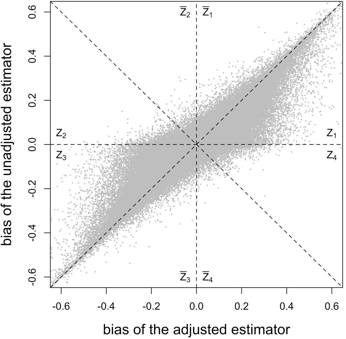 Figure 1
| Case | Z-Bias | |||||||||||
|---|---|---|---|---|---|---|---|---|---|---|---|---|
| 1 | 0.8 | 0.6 | 0.2 | 0.1 | 0.08 | 0.06 | 0.02 | 0.01 | 0.0550 | 0.0574 | 0.0584 | YES |
| 2 | 0.3 | 0.2 | 0.3 | 0.1 | 0.03 | 0.02 | 0.03 | 0.01 | 0.0050 | 0.0076 | 0.0077 | YES |
| 3 | 0.5 | 0.4 | 0.4 | 0.1 | 0.04 | 0.04 | 0.04 | 0.01 | 0.0150 | 0.0173 | 0.0172 | NO |
| point estimate | standard error | lower confidence limit | upper confidence limit | |
|---|---|---|---|---|
| 2.47 | 0.59 | 1.31 | 3.62 | |
| 1.77 | 0.07 | 1.64 | 1.90 | |
| 1.76 | 0.07 | 1.64 | 1.89 |
Peer Reviews
No public reviews on file for this paper yet. If you reviewed it on a platform where reviews are public (OpenReview, ICLR, NeurIPS, ICML), you can paste yours below so the community can read it here.
Videos
No videos yet. Explain this paper in a talk, walkthrough, or lecture? Add one.
Instrumental variables as bias amplifiers with general outcome and confounding
P. Ding
Department of Statistics, University of California, Berkeley, California, USA.
T. J. VanderWeele
J. M. Robins
Departments of Epidemiology and Biostatistics, Harvard T. H. Chan School of Public Health, Boston, Massachusetts, USA.
Abstract
Drawing causal inference with observational studies is the central pillar of many disciplines. One sufficient condition for identifying the causal effect is that the treatment-outcome relationship is unconfounded conditional on the observed covariates. It is often believed that the more covariates we condition on, the more plausible this unconfoundedness assumption is. This belief has had a huge impact on practical causal inference, suggesting that we should adjust for all pretreatment covariates. However, when there is unmeasured confounding between the treatment and outcome, estimators adjusting for some pretreatment covariate might have greater bias than estimators without adjusting for this covariate. This kind of covariate is called a bias amplifier, and includes instrumental variables that are independent of the confounder, and affect the outcome only through the treatment. Previously, theoretical results for this phenomenon have been established only for linear models. We fill in this gap in the literature by providing a general theory, showing that this phenomenon happens under a wide class of models satisfying certain monotonicity assumptions. We further show that when the treatment follows an additive or multiplicative model conditional on the instrumental variable and the confounder, these monotonicity assumptions can be interpreted as the signs of the arrows of the causal diagrams.
keywords:
Causal inference; Directed acyclic graph; Interaction; Monotonicity; Potential outcome
1 Introduction
Causal inference from observational data is an important but challenging problem for empirical studies in many disciplines. Under the potential outcomes framework (Neyman, 1923[1990]; Rubin, 1974), the causal effects are defined as comparisons between the potential outcomes under treatment and control, averaged over a certain population of interest. One sufficient condition for nonparametric identification of the causal effects is the ignorability condition (Rosenbaum & Rubin, 1983), that the treatment is conditionally independent of the potential outcomes given those pretreatment covariates that confound the relationship between the treatment and outcome. To make this fundamental assumption as plausible as possible, many researchers suggest that the set of collected pretreatment covariates should be as rich as possible. It is often believed that “typically, the more conditional an assumption, the more generally acceptable it is” (Rubin, 2009), and therefore “in principle, there is little or no reason to avoid adjustment for a true covariate, a variable describing subjects before treatment” (Rosenbaum, 2002, pp. 76).
Simply adjusting for all pretreatment covariates (d’Agostino, 1998; Rosenbaum, 2002; Hirano & Imbens, 2001), or the pretreatment criterion (VanderWeele & Shpitser, 2011), has a sound justification from the view point of design and analysis of randomized experiments. Cochran (1965), citing Dorn (1953), suggested that the planner of an observational study should always ask himself the question, “How would the study be conducted if it were possible to do it by controlled experimentation?” Following this classical wisdom, Rubin (2007, 2008a, 2008b, 2009) argued that the design of observational studies should be in parallel with the design of randomized experiments, i.e., because we balance all pretreatment covariates in randomized experiments, we should also follow this pretreatment criterion and balance or adjust for all pretreatment covariates when designing observational studies.
However, this pretreatment criterion can result in increased bias under certain data generating processes. We highlight two important classes of such data generating processes for which the pretreatment criterion may be problematic. The first class is captured by an example of Greenland & Robins (1986), in which conditioning on a pretreatment covariate invalidates the ignorability assumption and thus a conditional analysis is biased; yet the ignorability assumption holds unconditionally, so an analysis that ignores the covariate is unbiased. Several researchers have shown that this phenomenon is generic when the data are generated under the causal diagram in Figure 1(a). In this diagram, the ignorability assumption holds unconditionally but not conditionally (Pearl, 2000; Spirtes et al., 2000; Greenland, 2003; Pearl, 2009; Shrier, 2008, 2009; Sjölander, 2009; Ding & Miratrix, 2015). In Figure 1(a), a pretreatment covariate is associated with two independent unmeasured covariates and , but does not itself affect either the treatment or outcome . Because the corresponding causal diagram looks like the English letter M, this phenomenon is called M-Bias.
The second class of processes, which constitute the subject of this paper, are represented by the causal diagram in Figure 1(b). Owing to confounding by the unmeasured common cause of the treatment and the outcome , both the analysis that adjusts and the analysis that fails to adjust for pretreatment measured covariates are biased. If the magnitude of the bias is larger when we adjust for a particular pretreatment covariate than when we do not, we refer to the covariate as a bias amplifier. Of particular interest is to determine the conditions under which an instrumental variable is a bias amplifier. An instrumental variables is a pretreamtnet covariate that is independent of the confounder and has no direct effect on the outcome except through its effect on the treatment. The variable in Figure 1(b) is an example. Heckman & Navarro-Lozano (2004) and Bhattacharya & Vogt (2012) showed numerically that when the treatment and outcome are confounded, adjusting for an instrumental variable can result in greater bias than the unadjusted estimator. Wooldridge theoretically demonstrated this in linear models in a technical report in 2006, which was finally published as Wooldridge (2016). Because instrumental variables are often denoted by as in Figure 1(b), this phenomenon is called Z-Bias.
The treatment assignment is a function of the instrumental variable, the unmeasured confounder and some other independent random error, which are the three sources of variation of the treatment. If we adjust for the instrumental variable, the treatment variation is driven more by the unmeasured confounder, which could result in increased bias due to this confounder. Seemingly paradoxically, without adjusting for the instrumental variable, the observational study is more like a randomized experiment, and the bias due to confounding is smaller. Although applied researchers (Myers et al., 2011; Walker, 2013; Brooks & Ohsfeldt, 2013; Ali et al., 2014) have confirmed through extensive simulation studies that this bias amplification phenomenon exists in a wide range of reasonable models, definite theoretical results have been established only for linear models. We fill in this gap in the literature by showing that adjusting for an instrumental variable amplifies bias for estimating causal effects under a wide class of models satisfying certain monotonicity assumptions. When the instrumental variable and the confounder have either no additive or no multiplicative interaction on the treatment, these assumptions can be interpreted as the signs of the arrows of the causal diagram (VanderWeele & Robins, 2010). However, we also show that there exist data generating processes under which an instrumental variable is not a bias amplifier.
2 Framework and Notation
We consider a binary treatment , an instrumental variable , an unobserved confounder and an outcome , with the joint distribution depicted by the causal diagram in Figure 1(b). Let denote conditional independence between random variables. Then the instrumental variable in Figure 1(b) satisfies Z\begin{picture}(9.0,8.0)\put(0.0,0.0){\line(1,0){9.0}} \put(3.0,0.0){\line(0,1){8.0}} \put(6.0,0.0){\line(0,1){8.0}} \end{picture}U, Z\begin{picture}(9.0,8.0)\put(0.0,0.0){\line(1,0){9.0}} \put(3.0,0.0){\line(0,1){8.0}} \put(6.0,0.0){\line(0,1){8.0}} \end{picture}Y\mid(A,U) and Z\begin{picture}(9.0,8.0)\put(0.0,0.0){\line(1,0){9.0}} \put(3.0,0.0){\line(0,1){8.0}} \put(6.0,0.0){\line(0,1){8.0}} \put(1.0,0.0){{\it/}} \end{picture}A. We first discuss analysis conditional on observed pretreatment covariates , and comment on averaging over in §6 and the Supplementary Material. We define the potential outcomes of under treatment as , The true average causal effect of on for the population actually treated is
[TABLE]
for the population who are actually in the control condition it is
[TABLE]
and for the whole population it is
[TABLE]
Define to be the conditional mean of the outcome given the treatment and confounder. As illustrated by Figure 1(b), because suffices to control confounding between and , the ignorability assumption A\begin{picture}(9.0,8.0)\put(0.0,0.0){\line(1,0){9.0}} \put(3.0,0.0){\line(0,1){8.0}} \put(6.0,0.0){\line(0,1){8.0}} \end{picture}Y(a)\mid U holds for and . Therefore, according to , we have
[TABLE]
The unadjusted estimator is the naive comparison between the treatment and control means
[TABLE]
Define as the conditional mean of the outcome given the treatment and instrumental variable. Because the instrumental variable is also a pretreatment covariate unaffected by the treatment, the usual strategy to adjust for all pretreatment covariates suggests using the adjusted estimator for the population under treatment
[TABLE]
for the population under control
[TABLE]
and for the whole population
[TABLE]
Surprisingly, for linear structural equation models on , previous theory demonstrated that the magnitudes of the biases of the adjusted estimators are no smaller than the unadjusted ones (Pearl, 2010, 2011, 2013; Wooldridge, 2016). The goal of the rest of our paper is to show that this phenomenon exists in more general scenarios.
3 Scalar Instrumental Variable and Scalar Confounder
We first give a theorem for a scalar instrumental variable and a scalar confounder
Theorem 3.1**.**
In the causal diagram of Figure 1(b) with scalar and , if
- (a)
* is non-decreasing in , is non-decreasing in , and is non-decreasing in for both and ;* 2. (b)
* is non-increasing in for both and ,*
then
[TABLE]
Inequalities among vectors as in (1) should be interpreted as component-wise relationships. Intuitively, the monotonicity in Condition (a) of Theorem 3.1 requires non-negative dependence structures on arrows , and in the causal diagram of Figure 1(b). Because the dependence is in expectation, Condition (a) of Theorem 3.1 is weaker than the requirement of signed directed acyclic graphs (VanderWeele & Robins, 2010).
The monotonicity in Condition (b) of Theorem 3.1 reflects the collider bias caused by conditioning on . As noted by Greenland (2003), in many cases, if and affect in the same direction, then the collider bias caused by conditioning on is often in the opposite direction. Lemmas S6–S12 in the Supplementary Material show that, if and are independent and have non-negative additive or multiplicative effects on , then conditioning on results in negative association between and . This negative collider bias, coupled with the positive association between and , further implies negative association between and conditional on as stated in Condition (b) of Theorem 3.1.
For easy interpretation, we will give sufficient conditions for Z-Bias which require no interaction of and on When given and follows an additive model, we have the following theorem.
Theorem 3.2**.**
In the causal diagram of Figure 1(b) with scalar and , (1) holds if
- (a)
; 2. (b)
* is non-decreasing in , is non-decreasing in , and is non-decreasing in for both and [math];* 3. (c)
the essential supremum of given depends only on .
In summary, when given and follows an additive model and monotonicity of Theorem 3.2 holds, both unadjusted and adjusted estimators have non-negative biases for the true average causal effects for the treatment, control and the whole populations. Furthermore, the adjusted estimators, either for the treatment, control or the whole populations, have larger biases than the unadjusted estimator, i.e., Z-Bias arises.
When both the instrumental variable and the confounder are binary, Theorem 3.2 has an even more interpretable form. Define for and
Corollary 3.3**.**
In the causal diagram of Figure 1(b) with binary and , (1) holds if
- (a)
there is no additive interaction of and on , i.e., 2. (b)
* and have monotonic effects on , i.e., and , and for both and *
When given and follows an multiplicative model, we have the following theorem.
Theorem 3.4**.**
In the causal diagram of Figure 1(b) with scalar and , (1) holds if we replace Condition (a) of Theorem 3.2 by
- (a’)
.
When both the instrument and the confounder are binary, Theorem 3.4 can be simplified.
Corollary 3.5**.**
In the causal diagram of Figure 1(b) with binary and , (1) holds if we replace Condition (a) of Corollary 3.3 by
- (a’)
there is no multiplicative interaction of and on , i.e.,
We invoke the assumptions of no additive and multiplicative interaction of and on in Theorems 3.2 and 3.4 for easy interpretation. They are sufficient but not necessary conditions for Z-Bias. In fact, we show in the proofs that Conditions (a) and (a’) in Theorems 3.2 and 3.4 and Corollaries 3.3 and 3.5 can be replaced by weaker conditions. For the case with binary and , these conditions are particularly easy to interpret:
[TABLE]
i.e., and have non-positive multiplicative interaction on both the presence and absence of Even if Condition (a) or (a’) does not hold, one can show that half of the parameter space of satisfies the weaker condition (2), which is only sufficient, not necessary. Therefore, even in the presence of additive or multiplicative interaction, Z-Bias arises in more than half of the parameter space for binary .
4 General Instrumental Variable and General Confounder
When the instrumental variable and the confounder are vectors, Theorems 3.1–3.4 still hold if the monotonicity assumptions hold for each component of and , and and are multivariate totally positive of order two (Karlin & Rinott, 1980), including the case that the components of and are mutually independent (Esary et al., 1967). A random vector is multivariate totally positive of order two, if its density satisfies , where and are component-wise maximum and minimum of the vectors and . In the following, we will develop general theory for Z-Bias without the total positivity assumption about the components of and
It is relatively straightforward to summarize a general instrumental variable by a scalar propensity score , because Z\begin{picture}(9.0,8.0)\put(0.0,0.0){\line(1,0){9.0}} \put(3.0,0.0){\line(0,1){8.0}} \put(6.0,0.0){\line(0,1){8.0}} \end{picture}A\mid\Pi(Z) as shown in Rosenbaum & Rubin (1983). We define . The adjusted estimator for the population under treatment is
[TABLE]
the adjusted estimator for the population under control is
[TABLE]
and the adjusted estimator for the whole population is
[TABLE]
When is scalar, then the above three formulas reduce to the ones in Section 3.
Greenland & Robins (1986) showed that for the causal effect on the treated population, alone suffices to control for confounding; likewise, for the causal effect on the control population, alone suffices to control for confounding. If interest lies in all three of our average causal effects, then we need to take as the ultimate confounder for the relationship of on This is not an assumption about . Because is a deterministic function of and , this implies that satisfies the ignorability assumption (Rosenbaum & Rubin, 1983), or blocks all the back-door paths from to (Pearl, 1995, 2000). We represent the causal structure in Figure 2.
We first state a theorem without assuming the structure of the causal diagram in Figure 2.
Theorem 4.1**.**
*If for both and [math], is non-decreasing in , and , then (1) holds. *
In a randomized experiment A\begin{picture}(9.0,8.0)\put(0.0,0.0){\line(1,0){9.0}} \put(3.0,0.0){\line(0,1){8.0}} \put(6.0,0.0){\line(0,1){8.0}} \end{picture}Y(a), so the dependence of on characterizes the self-selection process of an observational study. The condition in Theorem 4.1 is another measure of the collider-bias caused by conditioning on , as and is a component of in Figure 2. This measure of collider bias is more general than the one in Theorem 3.1. Analogous to Section 3, we will present more transparent sufficient conditions for Z-Bias to aid interpretation.
In the following, we use the distributional association measure (Cox & Wermuth, 2003; Ma et al., 2006; Xie et al., 2008), i.e., random variable has a non-negative distributional association on random variable , if the conditional distribution satisfies for all and If the random variables are discrete, then partial differentiation is replaced by differencing between adjacent levels (Cox & Wermuth, 2003).
If there is no additive interaction between and on , then we have the following results.
Theorem 4.2**.**
In the causal diagram of Figure 2, (1) holds if
- (a)
* with and being non-decreasing;* 2. (b)
* have non-negative distributional associations on each other, i.e., and for all and ;* 3. (c)
the essential supremum of given does not depend on , and the essential supremum of given does not depend on .
Remark 4.3**.**
*If we impose an additive model then independence of and implies that Therefore, we must have and *
When the outcome is binary, the distributional association between and becomes their odds ratio (Xie et al., 2008), and non-negative distributional association between and is equivalent to
[TABLE]
We can further relax the model assumption of given and by allowing for non-negative interaction between and on
Corollary 4.4**.**
In the causal diagram of Figure 2 with a binary outcome , (1) holds if
- (a)
* with ;* 2. (b)
**
Remark 4.5**.**
If we have an additive model of given and , then the functional form imposes no restriction for binary outcome. Furthermore, implies that and , i.e., Therefore, the additive model in Condition (a) of Corollary 4.4 is
[TABLE]
If there is no multiplicative interaction of and on , then we have the following results.
Theorem 4.6**.**
In the causal diagram of Figure 2, (1) holds if we replace Condition (a) of Theorem 4.2 by
- (a’)
* with and being non-decreasing.*
Corollary 4.7**.**
In the causal diagram of Figure 2 with a binary outcome , (1) holds if we replace Condition (a) of Corollary 4.4 by
- (a’)
* with .*
5 Illustrations
5.1 Numerical Examples
Myers et al. (2011) simulated binary to investigate Z-Bias. They generated according to and . The first set of their generative models is additive,
[TABLE]
where the coefficients are all positive. The second set of their generative models is multiplicative,
[TABLE]
where the coefficients in (3) and (4) are all positive. They use simulation to show that Z-Bias arises under these models. In fact, in the above models, and have monotonic effects on without additive or multiplicative interactions, and acts monotonically on , given . Therefore, Corollaries 3.3 and 3.5 imply that Z-Bias must occur. The qualitative conclusion follows immediately from our theory. However, our theory does not make statements about the magnitude of the bias, and for more details about the magnitude and finite sample properties, see Myers et al. (2011).
We further use three numerical examples to illustrate the role of the no-interaction assumptions required by Theorems 3.2 and 3.4 and Corollaries 3.3 and 3.5. Recall the conditional probability of the treatment , , and define the conditional probabilities of the outcome as , for Table 1 gives three examples, where monotonicity on the conditional distributions of and hold, and there are both additive and multiplicative interactions. In all cases, the instrumental variable is Bernoulli, and the confounder is another independent Bernoulli. In Case 1, the weaker condition (2) holds, and our theory implies that Z-Bias arises. In Case 2, neither the condition in Theorem 3.1 or (2) holds, but Z-Bias still arises. Our conditions are only sufficient but not necessary. In Case 3, neither the condition in Theorem 3.1 or (2) holds, and Z-Bias does not arise.
Finally, for binary we use Monte Carlo to compute the volume of the Z-Bias space, i.e., the parameter space of , , ’s and ’s in which the adjusted estimator has higher bias than the unadjusted estimator. We randomly draw these ten probabilities from independent Uniform random variables, and for each draw of these probabilities we compute the average causal effect , the unadjusted estimator and the adjusted estimator . We plot the joint values of the biases in Figure 3. The volume of the Z-Bias space can be approximated by the frequency that deviates more from than . With random draws, our Monte Carlo gives an unbiased estimate for this volume as with estimated standard error . Therefore, in about of the parameter space, the adjusted estimator is more biased than the unadjusted estimator.
5.2 Real Data Examples
Bhattacharya & Vogt (2012) presented an example about the treatment effect of small classroom in the third grade on test scores for reading. Their instrumental variable analysis gave point estimate with standard error . Without adjusting for the instrumental variable in the propensity score model, the point estimate was with estimated standard error ; adjusting for the instrumental variable, the point estimate was with estimated standard error . The difference between the adjusted estimator and the instrumental variable estimator is larger than that between the unadjusted estimator and the instrumental variable estimator.
Wooldridge (2010, Example 21.3) discusses estimating the effect of attaining at least seven years of education on fertility, with treatment being a binary indicator for at least seven years of education, outcome being the number of living children, and instrumental variable being a binary indicator if the woman was born in the first half of the year. Although the original data set of Wooldridge (2010) contains other variables, most of them are posttreatment variables, so we do not adjust for them in our analysis. The instrumental variable analysis gives point estimate with estimated standard error . The unadjusted analysis gives point estimate with estimated standard error . The adjusted analysis gives point estimate with estimated standard error . Table 2 summarizes the results. In this example, the adjusted and unadjusted estimators give similar results.
6 Discussion
6.1 Allowing for an Arrow from to
When the variable has an arrow to the outcome as illustrated by Figure 4, the following generalization of Theorem 3.1 holds.
Theorem 6.1**.**
Consider the causal diagram of Figure 4 with scalar and , where Z\begin{picture}(9.0,8.0)\put(0.0,0.0){\line(1,0){9.0}} \put(3.0,0.0){\line(0,1){8.0}} \put(6.0,0.0){\line(0,1){8.0}} \end{picture}U and A\begin{picture}(9.0,8.0)\put(0.0,0.0){\line(1,0){9.0}} \put(3.0,0.0){\line(0,1){8.0}} \put(6.0,0.0){\line(0,1){8.0}} \end{picture}Y(a)\mid(Z,U) for and . The result in (1) holds if we replace Condition (a) of Theorem 3.1 by
- (a’)
* and are non-decreasing in and for and .*
However, when there is an arrow from to , Theorem 6.1 is of little use in practice without strong substantive knowledge about the size of the direct effect of on . In particular, neither Theorem 3.2 nor Theorem 3.4 is true when an arrow from to is present. This reflects the fact that neither the absence of an additive nor the absence of a multiplicative interaction of and on is sufficient to conclude that is non-increasing in when is non-decreasing in and .
With a general instrumental variable and a general confounder, Theorem 4.1 holds without any assumptions on the underlying causal diagram, and therefore it holds even if the variable affects the outcome directly. However, Theorems 4.2 and 4.6 no longer hold if an arrow from to is present as in Figure 4. This reflects the fact that the absence of an additive or multiplicative interaction of and on no longer implies when has a direct effect on , even if the remaining conditions of Theorems 4.2 and 4.6 hold. Analogously, Theorems 4.2 and 4.6 no longer hold if there exits an unmeasured common cause of and on the causal diagram in Figure 1(b), even if has no direct effect on .
6.2 Extensions
In §§2–4, we discussed Z-Bias for the average causal effects. We can extend the results to distributional causal effects for general outcomes (Ju & Geng, 2010) and causal risk ratios for binary or positive outcomes. Moreover, the results in §§2–4 are conditional on or within the strata of observed covariates. Similar results hold for causal effects averaged over observed covariates. We give more details in the Supplementary Material. In this paper we have given sufficient conditions for the presence of Z-Bias; future work could consider sufficient conditions for the absence of Z-Bias.
6.3 Conclusion
It is often suggested that we should adjust for all pretreatment covariates in observational studies. However, we show that in a wide class of models satisfying certain monotonicity, adjusting for an instrumental variable actually amplifies the impact of the unmeasured treatment-outcome confounding, which results in more bias than the unadjusted estimator. In practice, we may not be sure about whether a covariate is a confounder, for which one needs to control, or perhaps instead an instrumental variable, for which control would only increase any existing bias due to unmeasured confounding. Therefore, a more practical approach, as suggested by Rosenbaum (2010, Chapter 18.2) and Brookhart et al. (2010), may be to conduct analysis both with and without adjusting for the covariate. If two analyses give similar results, as in the example in Table 2, then we need not worry about Z-Bias; otherwise, we need additional information and analysis before making decisions.
Acknowledgments
Peng Ding is partially supported by the U.S. Institute of Education Sciences, and Tyler J. VanderWeele by the U.S. National Institutes of Health. The authors thank the Associate Editor and two reviewers for detailed and helpful comments.
Supplementary material
Supplementary Material available at Biometrika online includes all the proofs and extensions.
Appendix 1. Lemmas and Their Proofs
In order to prove the main results, we need to invoke the following lemmas. Some of them are from the literature, and some of them are new and of independent interest.
Lemma S2 is from Esary et al. (1967, Theorem 2.1).
Lemma S2**.**
*Let and be functions with real-valued arguments, which are both non-decreasing in each of their arguments. If is a multivariate random variable with mutually independent components, then *
Lemma S3 is from VanderWeele (2008), and Lemmas S4 and S5 are from Chiba (2009).
Lemma S3**.**
*For a univariate or a multivariate with mutually independent components, if for and [math], Y(a)\begin{picture}(9.0,8.0)\put(0.0,0.0){\line(1,0){9.0}} \put(3.0,0.0){\line(0,1){8.0}} \put(6.0,0.0){\line(0,1){8.0}} \end{picture}A\mid U, is non-decreasing in each component of , and is non-decreasing in each component of then and *
Lemma S4**.**
*For a univariate and a multivariate with mutually independent components, if Y(0)\begin{picture}(9.0,8.0)\put(0.0,0.0){\line(1,0){9.0}} \put(3.0,0.0){\line(0,1){8.0}} \put(6.0,0.0){\line(0,1){8.0}} \end{picture}A\mid U, is non-decreasing in each component of , and is non-decreasing in each component of then *
Lemma S5**.**
*For a univariate and a multivariate with mutually independent components, if Y(1)\begin{picture}(9.0,8.0)\put(0.0,0.0){\line(1,0){9.0}} \put(3.0,0.0){\line(0,1){8.0}} \put(6.0,0.0){\line(0,1){8.0}} \end{picture}A\mid U, is non-decreasing in each component of , and is non-decreasing in each component of then *
Lemma S6, extending Rothman et al. (2008), states that under monotonicity, no additive interaction implies non-positive multiplicative interactions for both presence and absence of the outcome.
Lemma S6**.**
If , , and , then
[TABLE]
Proof S7** (of Lemma S6).**
Define , and . Then implies which further implies
[TABLE]
The second inequality of (S5) follows from
[TABLE]
Lemma S6 is about interaction between two binary causes, and for our discussion we need to extend it to interaction between two general causes. Lemma S8 extends Piegorsch et al. (1994) and Yang et al. (1999) by relating the conditional association between two independent causes given the outcome to the interaction between the two causes on the outcome.
Lemma S8**.**
If Z\begin{picture}(9.0,8.0)\put(0.0,0.0){\line(1,0){9.0}} \put(3.0,0.0){\line(0,1){8.0}} \put(6.0,0.0){\line(0,1){8.0}} \end{picture}U, and with and non-decreasing in and , then for both and [math] and for all values of and ,
[TABLE]
*i.e., has non-positive distributional dependence on , given . *
Proof S9** (of Lemma S8).**
For a fixed and , we define
[TABLE]
following from the additive model of and Z\begin{picture}(9.0,8.0)\put(0.0,0.0){\line(1,0){9.0}} \put(3.0,0.0){\line(0,1){8.0}} \put(6.0,0.0){\line(0,1){8.0}} \end{picture}U.
Because it is straightforward to show that and . Because is increasing in , we have
[TABLE]
which imply and We further have
[TABLE]
The four probabilities satisfy the conditions in Lemma S6, Therefore, (2) holds. Replacing the probabilities in (2) by their definitions above, we have
[TABLE]
and
[TABLE]
Therefore, for both and [math] and for all values of ,
[TABLE]
is non-increasing in . Because of the independence of and , we have
[TABLE]
*Therefore, is a non-increasing function of (S6), and the conclusion holds. *
Lemmas S6 and S8 above hold under the assumption of no additive interaction, and the following two lemmas state similar results under the assumption of no multiplicative interaction.
Lemma S10**.**
If , and , then
[TABLE]
Proof S11** (of Lemma S10).**
Using the same notation in the proof of Lemma S6, implies , with , and Therefore,
[TABLE]
which further implies that
[TABLE]
Lemma S12**.**
If Z\begin{picture}(9.0,8.0)\put(0.0,0.0){\line(1,0){9.0}} \put(3.0,0.0){\line(0,1){8.0}} \put(6.0,0.0){\line(0,1){8.0}} \end{picture}U, and with and non-decreasing in and , then Z\begin{picture}(9.0,8.0)\put(0.0,0.0){\line(1,0){9.0}} \put(3.0,0.0){\line(0,1){8.0}} \put(6.0,0.0){\line(0,1){8.0}} \end{picture}U\mid A=1, and for all values of and ,
[TABLE]
*i.e., has non-positive distributional dependence on , given . *
Proof S13** (of Lemma S12).**
For a fixed and , we define
[TABLE]
following from the multiplicative model of and Z\begin{picture}(9.0,8.0)\put(0.0,0.0){\line(1,0){9.0}} \put(3.0,0.0){\line(0,1){8.0}} \put(6.0,0.0){\line(0,1){8.0}} \end{picture}U. Because we have and . Because is increasing in , we have
[TABLE]
which imply and We can further verify Because the four probabilities satisfy the conditions in Lemma S10, we have Replacing the probabilities by their definitions, we have
[TABLE]
*Following the same logic of the proof of Lemma S8, we can prove that Z\begin{picture}(9.0,8.0)\put(0.0,0.0){\line(1,0){9.0}} \put(3.0,0.0){\line(0,1){8.0}} \put(6.0,0.0){\line(0,1){8.0}} \end{picture}U\mid A=1, and has non-positive distributional association on , given . *
Define to be the proportion of the population under treatment. The average causal effect for the whole population can be written as a convex combination of the average causal effects for the treated and control populations:
[TABLE]
Analogously, with a scalar instrumental variable, the adjusted estimator for the whole population can be written as
[TABLE]
and with a general instrumental variable,
[TABLE]
Lemma S14**.**
With a scalar instrumental variable , the differences between the adjusted and unadjusted estimators are
[TABLE]
*With a general instrumental variable , the above formulas hold if we replace by and by *
Proof S15** (of Lemma S14).**
The difference is equal to
[TABLE]
Similarly, the difference is equal to
[TABLE]
Therefore, the difference is equal to
[TABLE]
*Analogously, we can prove the results for general instrumental variables. *
Appendix 2. Proofs of Theorems and Corollaries in the Main Text
Proof S16** (of Theorem 3.1).**
Because and are non-decreasing in and , and is non-decreasing in for both and , the unadjusted estimator, , is larger than or equal to and , according to Lemmas S3–S5.
Because is non-decreasing and is non-increasing in for both and , their covariance is non-positive according to Lemma S2, i.e.,
*Because the differences between all the adjusted estimators, , and , and the unadjusted estimator, , are negative constants multiplied by , according to Lemma S14 all of and are larger or equal to *
Proof S17** (of Theorem 3.2).**
The independence of and implies that
[TABLE]
are non-decreasing in and Therefore, according to Theorem 3.1 we need only to verify that in non-increasing in for both and
Because Z\begin{picture}(9.0,8.0)\put(0.0,0.0){\line(1,0){9.0}} \put(3.0,0.0){\line(0,1){8.0}} \put(6.0,0.0){\line(0,1){8.0}} \end{picture}U and with non-decreasing and , we can apply Lemma S8, and conclude that
Write the essential infimum and supremum of given as and , with the later depending only on according to Condition (c) of Theorem 3.2. Because Y\begin{picture}(9.0,8.0)\put(0.0,0.0){\line(1,0){9.0}} \put(3.0,0.0){\line(0,1){8.0}} \put(6.0,0.0){\line(0,1){8.0}} \end{picture}Z\mid(A,U), integration or summation by parts gives
[TABLE]
Therefore, its derivative with respect to ,
[TABLE]
*is smaller than or equal to zero, because for both and and for all . *
Proof S18** (of Corollary 3.3).**
*According to Theorem 3.1 we need only to verify that is non-increasing in for both and Following Lemma S6, for binary and independent and monotonicity and no additive interaction imply (S5), which, according to Bayes’ Theorem, is equivalent to *
[TABLE]
The above inequalities (S7) and (S8) state that and have negative association given each level of , and therefore is non-increasing in for both and
Because and
[TABLE]
*we know that is non-decreasing in . Therefore, is non-increasing in for both and *
Proof S19** (of Theorem 3.4).**
*Because of the independence of and , we have and are non-decreasing in and According to Lemma S12, the multiplicative model of also implies that for both and [math] and for all and , Following exactly the same steps of the proof of Theorem 3.2, we can prove Theorem 3.4. *
Proof S20** (of Corollary 3.5).**
For binary and independent and , monotonicity, no multiplicative interaction, and Lemma S10 imply
[TABLE]
*With the above results in (S9), the rest of the proof is the same as the proof of Corollary 3.3. *
Proof S21** (of Theorem 4.1).**
First, we consider the treatment effect on the population under treatment. Taking in Lemma S4, we have , because A\begin{picture}(9.0,8.0)\put(0.0,0.0){\line(1,0){9.0}} \put(3.0,0.0){\line(0,1){8.0}} \put(6.0,0.0){\line(0,1){8.0}} \end{picture}Y(0)\mid Y(0), is non-decreasing in , and is non-decreasing in . The condition implies that according to Lemma S14. Therefore,
Second, we take in Lemma S5, and by a similar argument as above we have
*The conclusion holds because and *
Proof S22** (of Theorem 4.2).**
Under the additive model of given and , we have the following results. First, is increasing in Second, \Pi\begin{picture}(9.0,8.0)\put(0.0,0.0){\line(1,0){9.0}} \put(3.0,0.0){\line(0,1){8.0}} \put(6.0,0.0){\line(0,1){8.0}} \end{picture}\{Y(1),Y(0)\} implies
[TABLE]
Denote the infimum and supremum of given by and , with the later not depending on according to Condition (c) of Theorem 4.2. Applying integration or summation by parts, we have
[TABLE]
The function is non-decreasing in , because
[TABLE]
Third, following the same reasoning as the second argument, we have with being a non-decreasing function of Fourth, \Pi\begin{picture}(9.0,8.0)\put(0.0,0.0){\line(1,0){9.0}} \put(3.0,0.0){\line(0,1){8.0}} \put(6.0,0.0){\line(0,1){8.0}} \end{picture}Y(1) implies which is non-decreasing in Fifth, \Pi\begin{picture}(9.0,8.0)\put(0.0,0.0){\line(1,0){9.0}} \put(3.0,0.0){\line(0,1){8.0}} \put(6.0,0.0){\line(0,1){8.0}} \end{picture}Y(0) implies which is non-decreasing in
According the fourth and fifth arguments above, Condition (a) in Theorem 4.1 holds. Therefore, we need only to verify Condition (b) in Theorem 4.1 to complete the proof.
We have shown that , which is additive and non-decreasing in and . According to Lemma S8, we know that
[TABLE]
for all and We have also shown that , which is additive and non-decreasing in and . Again according to Lemma S8, we know that
[TABLE]
*for all and According to Xie et al. (2008), the above negative distributional associations in (S10) and (S11) imply the negative associations in expectation between and given , as required by condition (b) of Theorem 4.1. *
Proof S23** (of Corollary 4.4).**
As shown in the proof of Theorem 4.2, the conclusion follows immediately from the five ingredients. We will show that they hold even if there is non-negative interaction between binary and . The following proof is in parallel with the proof of Theorem 4.2.
First, is increasing in Second,
[TABLE]
The last equation in (S13) follows from the fact that is binary and the functional form must be linear in , where the coefficient is
[TABLE]
where (LABEL:eq::coef-given-y1) follows from (S12), and (S15) follows from and Because , the potential outcomes have non-negative association, implying that their risk difference . Therefore, , and is additive and non-decreasing in and .
Third, similar to the second argument, we have with Therefore, is additive and non-decreasing in and . Fourth, \Pi\begin{picture}(9.0,8.0)\put(0.0,0.0){\line(1,0){9.0}} \put(3.0,0.0){\line(0,1){8.0}} \put(6.0,0.0){\line(0,1){8.0}} \end{picture}Y(1) implies that is increasing in Fifth, \Pi\begin{picture}(9.0,8.0)\put(0.0,0.0){\line(1,0){9.0}} \put(3.0,0.0){\line(0,1){8.0}} \put(6.0,0.0){\line(0,1){8.0}} \end{picture}Y(0) implies that is increasing in
*With these five ingredients, the rest of the proof is exactly the same as the proof of Theorem 4.2. *
Proof S24** (of Theorem 4.6).**
First, is non-decreasing in . Second,
[TABLE]
is multiplicative and non-decreasing in and , following the same argument as the proof of Theorem 4.2. Third, is multiplicative and non-decreasing in and . Fourth, is non-decreasing in . Fifth, is non-decreasing in .
The multiplicative models and Lemma S12 imply that for all and ,
[TABLE]
*The rest part is the same as the proof of Theorem 4.2. *
Proof S25** (of Corollary 4.7).**
First, is non-decreasing in . Second,
[TABLE]
where the functional form must be multiplicative because of binary , and the parameter is
[TABLE]
Because , we have , which implies that Therefore, is multiplicative and non-decreasing in and . Third, we can similarly show that is multiplicative and non-decreasing in and Fourth, is non-decreasing in . Fifth, is non-decreasing in .
*The rest part is the same as the proof of Theorem 4.6. *
Proof S26** (of Theorem 6.1.).**
In Figure 4, and are two independent confounders for the relationship between and . Because and are non-decreasing in and for both and , Lemmas S3–S5 imply that the unadjusted estimator, , is larger than or equal to and .
*The independence between and implies , and the monotonicity of in implies that is non-decreasing in . The rest of the proof is identical to the proof of Theorem 3.1. *
Appendix 3. Extensions to Other Causal Measures
Appendix 31. Distributional Causal Effects
Sometimes we are also interested in estimating the distributional causal effects (Ju & Geng, 2010) for the treatment, control and whole populations:
[TABLE]
The unadjusted estimator is
[TABLE]
The adjusted estimators for the treatment, control and whole populations are
[TABLE]
If the outcome is binary, then the distributional causal effects at are the average causal effects, and zero at . All results about distributional causal effects reduce to average causal effects for binary outcome. For a general outcome, the distributional causal effects are the average causal effects on the dichotomized outcome Therefore, if we replace the outcome by in Theorems 3.1–3.4, the results about Z-Bias hold for distributional effects. For instance, the condition that is non-decreasing in for all is the same as requiring a non-negative sign on the arrow , according to the theory of signed directed acyclic graphs (VanderWeele & Robins, 2010). The following theorem states the results analogous to Theorems 4.1–4.6.
Corollary S27**.**
In the causal diagram of Figure 2, if for all and for both and [math],
- (a)
; 2. (b)
;
then
[TABLE]
*Under the conditions of Theorems 4.2 and 4.6, (S17) holds. *
Proof S28** (of Corollary S27).**
Condition (a) of Corollary S27 is equivalent to , and Condition (b) of Corollary S27 is equivalent to . Therefore, the conclusion follows from Theorem 4.1.
According to the proofs of Theorems 4.2 and 4.6, we have
[TABLE]
*because of monotonicity of in . Therefore, Condition (a) of Theorem S27 holds. Under the conditions of Theorems 4.2 and 4.6, we have also shown in (S10)–(S16) that for all and , which implies that is non-increasing in . Therefore, Condition (b) of Theorem S27 holds. The proof is complete. *
Appendix 32. Ratio Measures
In many applications with binary or positive outcomes, we are also interested in assessing causal effects on the ratio scale for the treatment, control and whole populations, defined as
[TABLE]
The unadjusted estimator on the ratio scale is
[TABLE]
The adjusted estimators on the ratio scale for the treatment, control and whole populations are
[TABLE]
With a general instrumental variable , we can replace by in the definitions of the adjusted estimators.
Corollary S29**.**
All the theorems and corollaries in §§3 and 4 hold on the ratio scale, i.e., under their conditions,
[TABLE]
Proof S30** (of Corollary S29).**
*First, is a convex combination of and , and is a convex combination of and , which are formally stated in Ding & VanderWeele (2016, eAppendix). Then the conclusion follows from the proofs of the theorems above. *
Appendix 33. Average Over Observed Covariates
In practice, we need to adjust for the observed covariates that are confounders affecting both the treatment and outcome. The discussion in previous sections is conditional on or within strata of observed covariates , and the causal effects and their estimators are given . For example,
[TABLE]
and other conditional quantities can be analogously defined. If the conditions in the theorems and corollaries in §§3 and 4 hold within each level of , then the conclusions in (1) and (S17) hold not only within each level of but also averaged over . For example, for the average causal effects, we have
[TABLE]
The reference list from the paper itself. Each links out to its DOI / PubMed record.
- 1Ali et al. (2014) Ali, M. S. , Groenwold, R. H. & Klungel, O. H. (2014). Propensity score methods and unobserved covariate imbalance: Comments on “Squeezing the balloon”. Health Services Research 49 , 1074–1082.
- 2Bhattacharya & Vogt (2012) Bhattacharya, J. & Vogt, W. B. (2012). Do instrumental variables belong in propensity scores? Int. J. Stat. Econ. 9 , 107–127.
- 3Brookhart et al. (2010) Brookhart, M. A. , Stürmer, T. , Glynn, R. J. , Rassen, J. & Schneeweiss, S. (2010). Confounding control in healthcare database research: challenges and potential approaches. Medical Care 48 , S 114–S 120.
- 4Brooks & Ohsfeldt (2013) Brooks, J. M. & Ohsfeldt, R. L. (2013). Squeezing the balloon: Propensity scores and unmeasured covariate balance. Health Services Research 48 , 1487–1507.
- 5Chiba (2009) Chiba, Y. (2009). The sign of the unmeasured confounding bias under various standard populations. Biometrical Journal 51 , 670–676.
- 6Cochran (1965) Cochran, W. G. (1965). The planning of observational studies of human populations (with discussion). Journal of the Royal Statistical Society: Series A (General) 128 , 234–266.
- 7Cox & Wermuth (2003) Cox, D. & Wermuth, N. (2003). A general condition for avoiding effect reversal after marginalization. Journal of the Royal Statistical Society: Series B (Statistical Methodology) 65 , 937–941.
- 8d’Agostino (1998) d’Agostino, R. B. (1998). Tutorial in biostatistics: Propensity score methods for bias reduction in the comparison of a treatment to a non-randomized control group. Statistics in Medicine 17 , 2265–2281.