Finite-key analysis for quantum key distribution with weak coherent pulses based on Bernoulli sampling
Shun Kawakami, Toshihiko Sasaki, Masato Koashi

TL;DR
This paper introduces a Bernoulli sampling-based parameter estimation method for finite-key quantum key distribution, improving key rates for BB84 with weak coherent pulses and confirming the finite-key advantage of the DQPS protocol.
Contribution
It proposes a concise Bernoulli sampling method for finite-key analysis, reducing parameter estimation complexity and enhancing key rates in quantum key distribution protocols.
Findings
Bernoulli sampling improves parameter estimation efficiency.
The method increases the key rate for BB84 with weak coherent pulses.
Finite-key security of the DQPS protocol is established, confirming its advantage.
Abstract
An essential step in quantum key distribution is the estimation of parameters related to the leaked amount of information, which is usually done by sampling of the communication data. When the data size is finite, the final key rate depends on how the estimation process handles statistical fluctuations. Many of the present security analyses are based on the method with simple random sampling, where hypergeometric distribution or its known bounds are used for the estimation. Here we propose a concise method based on Bernoulli sampling, which is related to binomial distribution. Our method is suitable for the BB84 protocol with weak coherent pulses, reducing the number of estimated parameters to achieve a higher key generation rate compared to the method with simple random sampling. We also applied the method to prove the security of the differential-quadrature-phase-shift (DQPS) protocol…
Click any figure to enlarge with its caption.
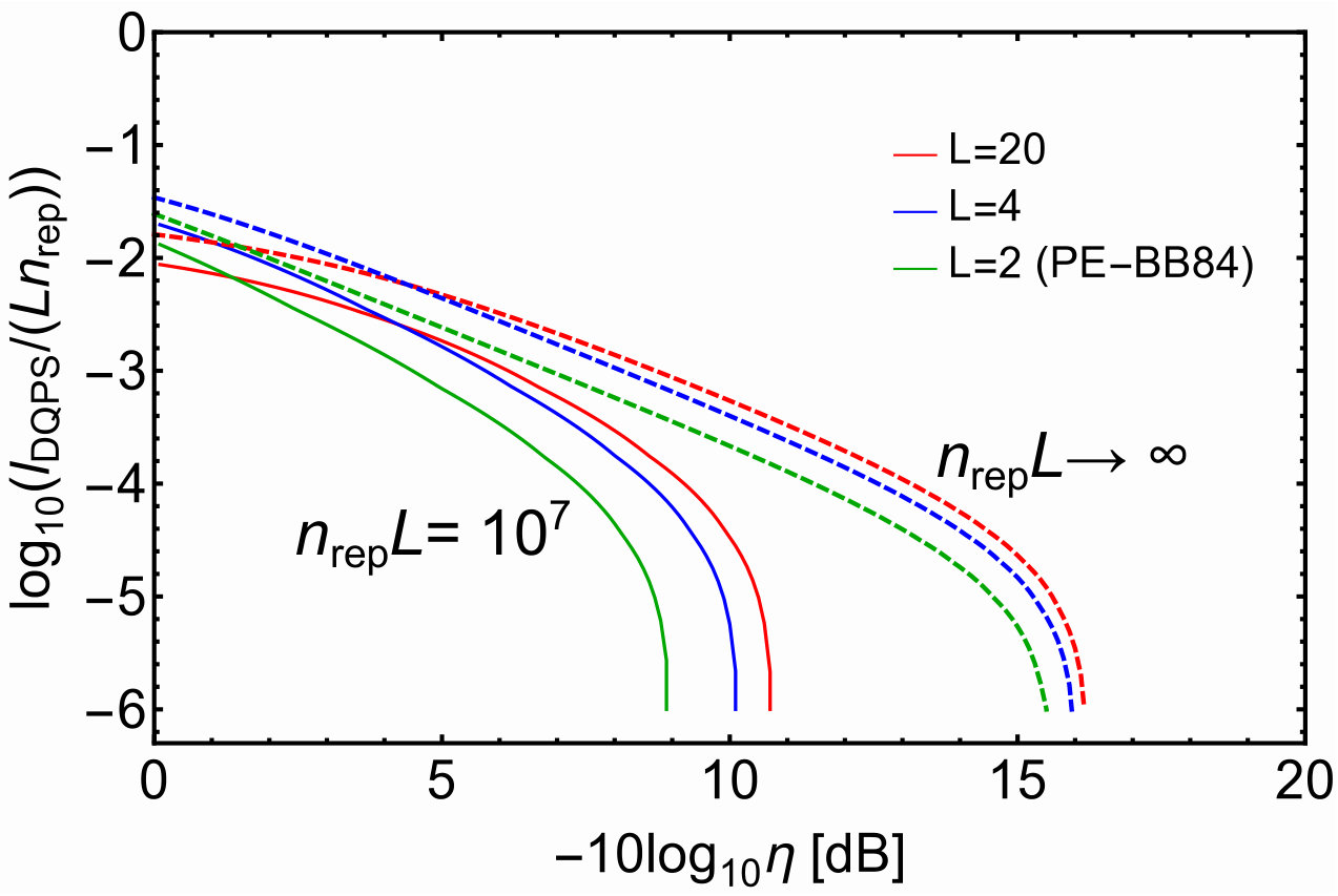 Figure 1
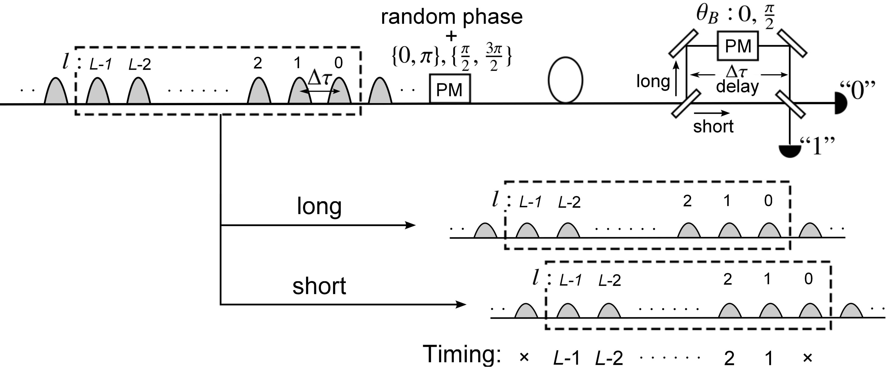 Figure 3
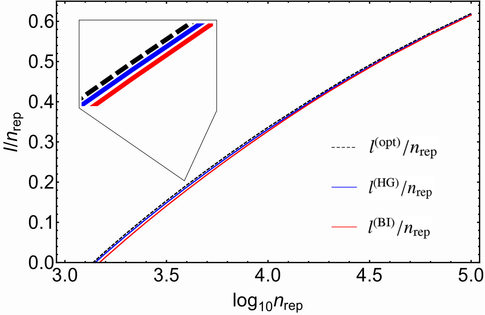 Figure 3
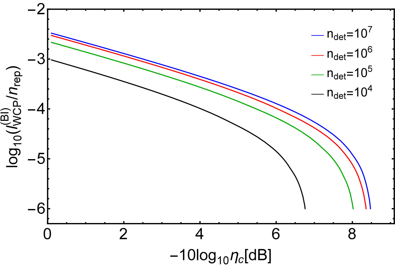 Figure 4
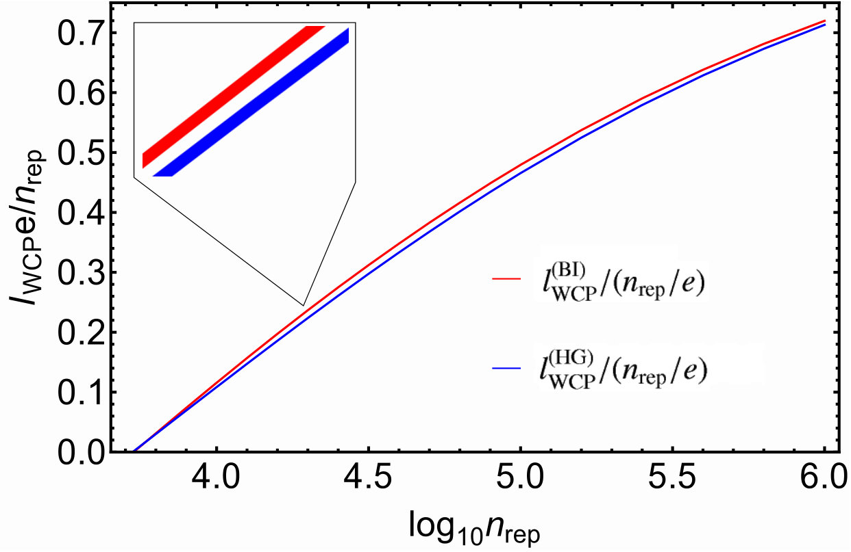 Figure 5
Peer Reviews
No public reviews on file for this paper yet. If you reviewed it on a platform where reviews are public (OpenReview, ICLR, NeurIPS, ICML), you can paste yours below so the community can read it here.
Videos
No videos yet. Explain this paper in a talk, walkthrough, or lecture? Add one.
Finite-key analysis for quantum key distribution with weak coherent pulses
based on Bernoulli sampling
Shun Kawakami1,2, Toshihiko Sasaki1 and Masato Koashi1,2
1Photon Science Center, Graduate School of Engineering, The University of Tokyo, 2-11-16 Yayoi, Bunkyo-ku, Tokyo 113-8656, Japan
2 Department of Applied Physics, Graduate School of Engineering, The University of Tokyo, 7-3-1 Hongo, Bunkyo-ku, Tokyo 113-8656, Japan
Abstract
An essential step in quantum key distribution is the estimation of parameters related to the leaked amount of information, which is usually done by sampling of the communication data. When the data size is finite, the final key rate depends on how the estimation process handles statistical fluctuations. Many of the present security analyses are based on the method with simple random sampling, where hypergeometric distribution or its known bounds are used for the estimation. Here we propose a concise method based on Bernoulli sampling, which is related to binomial distribution. Our method is suitable for the BB84 protocol with weak coherent pulses, reducing the number of estimated parameters to achieve a higher key generation rate compared to the method with simple random sampling. We also applied the method to prove the security of the differential-quadrature-phase-shift (DQPS) protocol in the finite-key regime. The result indicates that, the advantage of the DQPS protocol over the phase-encoding BB84 protocol in terms of the key rate, which was previously confirmed in the asymptotic regime, persists in the finite-key regime.
pacs:
03.67.Dd, 03.67.Hk.
I Introduction
Quantum key distribution (QKD) allows two distant parties to share a secret key and realizes a communication with information-theoretic security by combining it with one-time-pad encryption. Since the BB84 protocol was proposed by Bennett and Brassard Bennett and Brassard (1984a), a large number of researches on QKD have been conducted from both aspects of theory and implementations. The security of QKD is based only on principles of quantum physics where eavesdropped information is bounded from the observed parameters in a protocol. In practice, the estimation of this bound should take into account statistical fluctuations due to the finite size of communication data, which requires so-called finite-key analysis. Following the security definition with composability Ben-Or et al. (2005); Renner and Konig (2005), the finite-key analyses for various QKD protocols including the BB84 protocol were conducted assuming the adversary’s general attacks Tomamichel et al. (2012); Furrer et al. (2012); Lim et al. (2014); Curty et al. (2014); Hayashi and Nakayama (2014); Lucamarini et al. (2015); Mizutani et al. (2015).
For a finite-key analysis, a simple method with a smaller number of estimation processes is preferred because it leads not only to a more concise security proof but also to a higher key-generation rate especially when the number of communication rounds is limited and statistical fluctuations are large. A number of recent finite-key analyses are based on the method with simple random sampling, which is used to model draws, without replacement, from a finite population of size that contains errors. The probability that the number of errors in the sample is obeys hypergeometric distribution
[TABLE]
In several finite-key analyses Hayashi and Nakayama (2014); Lucamarini et al. (2015) based on simple random sampling, efforts were made to find bounds on hypergeometric distribution which are related to binomial distribution in order to simplify numerical calculation.
In order to mitigate the inefficiency arising from basis mismatch between the sender and the receiver, the BB84 protocol is often implemented with biased basis choice Lo et al. (2004), in which the minor basis is used solely for monitoring leaked information in the major basis. In this case, the whole data from the rounds in the monitoring basis is regarded as a sample, with each round selected with a constant probability dictated in the protocol as that of the basis choice. This suggests that the data from the monitoring basis is related to Bernoulli sampling, in which each element of the population of size is sampled with fixed probability . The number of samples obeys binomial distribution
[TABLE]
If the BB84 protocol with biased basis choice essentially includes the property of the binomial distribution, analysis based on the conventional simple random sampling may introduce unnecessary complexity and possibly leads to a lower key rate.
In this paper, we work on the finite-key analysis by focusing on the Bernoulli sampling instead of simple random sampling. We propose the method based on binomial distribution which is parametrized by the basis choice probabilities in the protocol. Differently from the previous works which deal with binomial distribution to derive bounds on hypergeometric distribution, our work is based on binomial distributions inherent in the protocol. Our method is especially suited for the BB84 protocol with weak coherent pulses (WCP), providing a simpler analysis with less estimation processes as well as achieving a higher key rate compared to the analysis with simple random sampling. We further apply this method to the differential quadrature phase shift (DQPS) protocol Inoue and Iwai (2009), whose security was proved recently in the asymptotic regime Kawakami et al. (2016). As a result, we show that the advantage of the DQPS protocol over the phase-encoded BB84 protocol with WCP still remains in the finite key regime.
This paper is organized as follows. In Sec. II, we describe details of the BB84 protocol which is considered in this work, along with a summary of notations used in this paper. In Sec. III, we propose a method of finite-key analysis based on Bernoulli sampling, and applies it to the ideal BB84 protocol where Alice and Bob can manipulate perfect single photon states. The proposed method is then applied to the BB84 protocol with WCP as well as the DQPS protocol in Sec. IV.1. Finally, we give discussion and conclusion in Sec. V.
II BB84 Protocol
In most part of this paper, we discuss the finite key analysis of the BB84 protocol Bennett and Brassard (1984b), which is given in the following. The sender Alice and the receiver Bob independently chooses two bases ( basis and basis) with a biased probability. The final key is generated only from -basis data, while -basis data is used for leak monitoring to determine the amount for privacy amplification. The number of total rounds are predetermined and there is no threshold for data size after sifting process, which means that the size of sifted key and that of monitoring bits are not determined until quantum communication is over.
The protocol proceeds as follows with predetermined parameters , and . In its description, represents the length of a bit sequence .
(1) Alice chooses basis or basis with probability and , respectively. She chooses a uniformly random bit .
(2) Alice prepares one of states based on the selected basis and bit. She sends the prepared state to Bob over the quantum channel.
(3) Bob chooses basis or basis with probability and , respectively. He measures a received state in chosen basis and obtains the outcome {0, 1, no-detection}.
(4) They repeat the sequence (1) to (3), which we call a round, by times.
(5) Bob publicly announces whether each round has resulted in a detection or not. Let be the number of rounds with detection.
(6) Alice and Bob disclose all of their basis choices. Among the detected rounds, the rounds where both Alice and Bob chose the basis are called “-labeled” rounds, and the rounds where they chose the basis are called “-labeled” rounds. They define sifted keys and by concatenating the bits for the -labeled rounds, and similarly define and for the -labeled rounds. Let their sizes be and .
(7) They disclose and compare and to determine the number of bit errors included in them.
(8) Through public discussion, Bob corrects his keys to make it coincide with Alice’s key and obtains .
(9) Alice and Bob conduct privacy amplification by shortening and to obtain final keys and of size .
In the subsequent sections, we discuss how we can determine the final key length as a function of the random variables , , and obtained in the protocol to satisfy a given security criteria. For convenience, we define several variables and parameters as and
[TABLE]
Throughout this paper, we adopt an abuse of notation to use the same symbol for a random variable and its value , whenever the distinction is obvious. For example, we denote instead of . We denote by the probability mass function . Similarly, we use instead of . We define and as basis vectors of basis on a qubit system, and and as those of basis. When the same notations are used for an optical signal, it should be understood that they refer to the states in the subspace of a single photon contained in two modes, such as polarizations. The four Bell sates are represented as and where
[TABLE]
We define a function for as
[TABLE]
III Analysis for the ideal BB84 protocol
Here we consider finite-key analysis for the ideal qubit-based BB84 protocol, in which Alice sends a single photon in the states in Step (2) and Bob conducts ideal measurement with unit efficiency described by POVM (positive operator-valued measure) corresponding to the outcome {0,1,no-detection}.
III.1 Security criteria and formalism for key length
In this work, we follow the security definition based on universally composable security Ben-Or et al. (2005); Renner and Konig (2005). The protocol is called secure if it is both -correct and -secret where . We call the protocol is -correct if holds. We call the protocol is -secret if
[TABLE]
where is a classical-quantum state between Alice’s key and Eve’s system after finishing the protocol and is an ideal separable state in which Alice’s key is uniformly distributed over values and decoupled from Eve’s system.
In the ideal BB84 protocol, Alice’s procedure of selecting a random bit and a basis, and preparing the corresponding signal can be replaced Bennett et al. (1992) by preparation of followed by the measurement on the system on (-basis) or on (-basis). Bob’s measurement is also replaced by a filtering operation to make sure a single photon is received and transfer its state to a qubit , followed by the orthogonal measurement of on the chosen basis to determine the outcome 0 or 1. When the filtering fails, the outcome is “no-detection”. According to Ref. Lo and Chau (1999); Shor and Preskill (2000), a phase error occurs when Alice and Bob conduct virtual Bell-basis measurement on a -labeled round after Eve’s intervention to obtain the outcome for or . Since we have the relation
[TABLE]
phase error is equivalently defined as a bit error which occurs when Alice and Bob conduct virtual -basis measurement after Eve’s intervention on a -labeled round. An important property which will be used in the next subsection is that the measurement for a phase error on a -labeled round and the measurement for a bit error on an -labeled round are identical, and hence they only differs in the labeling.
Let be a random variable which represents the number of phase errors on -labeled rounds. Once we have a good upper bound on , a secure key length can be calculated as follows. Suppose that we have a function which satisfies
[TABLE]
regardless of Eve’s attack strategy. By setting Hayashi and Nakayama (2014)
[TABLE]
the protocol is -correct and -secret if the final key length satisfies
[TABLE]
where represents the ceiling function and is the cost of error correction to achieve -correctness. For simplicity, we will replace the right-hand side by a slightly pessimistic bound as
[TABLE]
III.2 Bounds on phase errors
In this subsection, we discuss the specific methods to obtain in Eq. (9) including a method based on the Bernoulli sampling, and a more conventional method based on the simple random sampling. We also introduce a third, rather convoluted method, which will help to elucidate the difference between the former two methods.
Before discussing each of the methods, we first derive general statistical properties. Since the -labeled phase error and the -labeled bit error are obtained by identical measurements, the procedure to obtain those errors is equivalent to the following steps after discarding the rounds with no-detection (i.e., with Bob failing to receive a qubit): (a) Alice and Bob further discard each of the remaining rounds with probability . (b) They make -basis measurements on the remaining rounds and obtain errors. (c) Finally, they label each of the rounds as or with probability and (see Eq. (3)), respectively, and obtain phase errors in -labeled rounds and bit errors in -labeled rounds. In this procedure, since errors are sampled from errors with a fixed probability , it follows a binomial distribution if and are fixed:
[TABLE]
On the other hand, the step (c) of the above procedure is equivalently denoted as follows: Alice and Bob draw a number based on the binomial distribution , and then select random rounds among the rounds to label as , thereby determining . This implies that the number obeys hypergeometric distribution if , and are fixed:
[TABLE]
In order to use the properties derived above, it is convenient to reformulate Eq. (9) as follows. From Eq. (9), we have
[TABLE]
Since can be under control of Eve, we seek for satisfying
[TABLE]
for any and , which is a sufficient condition for Eq. (9). For later convenience, we equivalently describe Eq. (16) as
[TABLE]
The first method to determine , whose utility we will emphasize throughout this paper, is based on Bernoulli sampling using the property of binomial distribution Eq. (13). This method adopts where
[TABLE]
The proof that satisfies Eq. (16) is as follows. Let \overline{\hbox{k}}_{X}(k_{\rm tot}):={\rm max}\{k_{X}\mid k_{\rm tot}>f_{\rm BI}(k_{X})+k_{X}\}. Then we have
[TABLE]
Since is a decreasing function of , from Eq. (18) we have for any pair satisfying . Since k_{\rm tot}\geq f_{\rm BI}(\overline{\hbox{k}}_{X}(k_{\rm tot}))+\overline{\hbox{k}}_{X}(k_{\rm tot})+1 holds by definition of \overline{\hbox{k}}_{X}(k_{\rm tot}), we have C_{\rm BI}(\overline{\hbox{k}}_{X}(k_{\rm tot});k_{\rm tot},p_{X})\leq\epsilon_{\rm PE}. By connecting this to Eq. (20), we have
[TABLE]
for any . From Eqs. (13) and (21), we have
[TABLE]
which is identical to Eq. (17) with . Therefore, we have
[TABLE]
As a result of the Bernoulli-sampling method, the protocol is -correct and -secret if the final key length satisfies
[TABLE]
where is given by Eq. (10).
The second method is based on simple random sampling, applying the property of the hypergeometric distribution Eq. (14), which is already seen in Ref. Tomamichel et al. (2012); Lim et al. (2014); Curty et al. (2014); Hayashi and Nakayama (2014), for example. This method adopts where
[TABLE]
The proof that satisfies Eq. (16) is similar to the proof for . Recall that the proof for did not use the explicit form of but only used the decreasing property of as a function of . Since is also a decreasing function of , we have
[TABLE]
for any , and , which is analogous to Eq. (21). From Eqs. (14) and (26), we have
[TABLE]
which is identical to Eq. (17) with . Therefore, we have
[TABLE]
As a result of the method with simple random sampling, the protocol is -correct and -secret if the secret key length satisfies
[TABLE]
where is given by Eq. (10).
To understand the relation between the two methods with Bernoulli sampling and simple random sampling, we introduce another method which uses full knowledge of the distribution appearing in Eq. (17). The argument before Eq. (13) also implies that the number of -labeled rounds without bit error obeys binomial distribution , and that and are independent conditioned on and . We thus obtain
[TABLE]
The argument leading to Eq. (14) gives another expression for the distribution as
[TABLE]
As a result, Eq. (17) is expressed in the following two equivalent ways:
[TABLE]
or
[TABLE]
Since satisfies Eq. (21), Eq. (LABEL:ikko) holds if . Similarly, since satisfies Eq. (26), Eq. (33) holds if . On the other hand, the condition of Eqs. (LABEL:ikko) and (33) do not imply Eq. (21) or Eq. (26). Therefore, there could be a better bound compared to and based on Eq. (LABEL:ikko) or Eq. (33). In general, it is very complicated to determine the optimal function for the final key length , since it will depend on the explicit functional dependence of on .
The difference between the two equivalent conditions Eqs. (LABEL:ikko) and (33) is the choice of two variables from three no-independent random variables , and . When are chosen in Eq. (33), the distribution of , is dependent on the value of . On the other hand, Eq. (LABEL:ikko) implies that two variables are independent of each other. This suggests that the underlying statistics in the BB84 protocol with biased basis choice are understood in terms of independent binomial distributions.
Let us mention the difference from the other works Hayashi and Nakayama (2014); Lucamarini et al. (2015) which deal with relations between bounds on binomial distribution and ones on hypergeometric distribution since the former are easily treated with existing mathematical packages. Ref. Hayashi and Nakayama (2014) uses the property, which dates back to Hoeffding Hoeffding (1963), that expectation of a convex function over hypergeometric dirstribution is no larger than that over binomial distribution. In Lucamarini et al. (2015), Ahrens map Ahrens (1987) was used to show that hypergeometric dirstribution is bounded by a permutated binomial distribution within a factor of . In contrast to these works, in our case the probability distribution Eq. (13) reflects the binomial distribution inherent in the BB84 protocol with biased basis choice.
III.3 Numerical examples
Here we numerically compare the final key lengths derived from the three methods in the last subsection in the simplest cases. We calculate the key lengths for the case where no error is observed () and every signal is detected (. The cost of error correction is set to . We also assume and .
If we do not care about the key length for , the optimal choice of satisfying Eq. (33) (or Eq. (LABEL:ikko)) is given by for and with
[TABLE]
The proof is analogous to the one for or . Since is a decreasing function of , by using an argument similar to the one leading to Eq. (21), we have
[TABLE]
This is identical to Eq. (33) since is never satisfied for . The key length when was observed is then given by
[TABLE]
In Fig. 1, we show the secure key ratios to the asymptotic case , and as functions of total rounds of the protocol . For each , the value of was optimized to maximize the key length. In the limit of , each curve converges to . The security parameters are set to and , and . We see that although the key rate is the best, the three methods achieve almost the same key length.
IV Analysis for WCP-based protocol
Here, we apply the analyses introduced in the previous section to the protocols using weak coherent pulses (WCP). We consider the WCP-based BB84 protocol in the subsections A and B, and move to the DQPS protocol in subsection C.
IV.1 The WCP-BB84 protocol
Similarly to the ideal qubit-based protocol, the WCP-BB84 protocol also follows the procedures described in Sec. II, but the latter assumes more general light sources and measurement apparatuses. We prove the security of the WCP-BB84 protocol based on that of qubit-based BB84 protocol combined with GLLP’s tagging idea Gottesman et al. (2004). We impose the following assumptions on Alice and Bob’s devices. For Alice’s light source, we assume that the four states with and are written as
[TABLE]
For , we assume that there is a basis-independent state on the system satisfying
[TABLE]
We place no restriction on the states . We may still find a state on the system such that
[TABLE]
but depends on a selected basis . The form of Eq. (37) allows an interpretation that each round is classified as either tagged or untagged Gottesman et al. (2004). The density operator is the state of Alice’s untagged signal which may generate a secure key and is that of her tagged signal which is considered to be totally insecure. Equation (38) indicates that Alice’s basis choice can be postponed until Bob receives the system for untagged rounds. Eqs. (37) and (38) are realized, for example, if Alice uses a laser emitting an ideally polarized coherent pulse with mean photon number and randomizes its optical phase. In this case, and are written as
[TABLE]
where is an -photon state with a basis and a bit , and
[TABLE]
represents the probability that Alice emits two or more photons. Our proof does not depend on the specific model such as coherent light source, but depends only on Eqs. (37) and (38).
For Bob’s measurement apparatus, we impose either of the following two assumptions.
(i) The probability of detecting a signal at Bob’s receiver is independent of his basis choice.
(ii) The measurement of an input signal on the system is replaced by an ideal single-photon measurement on the system preceding by a squashing operation Tsurumaru and Tamaki (2008); Beaudry et al. (2008).
The condition (i), which is weaker than condition (ii), allows us to use the security proof with complementarity Koashi (2009) and uncertainty principle Tomamichel et al. (2012). The condition (ii) validates the use of the security proof with entanglement distillation Shor and Preskill (2000). For the WCP-BB84 protocol, both conditions are satisfied if we assume the following model for Bob’s apparatus: Bob actively chooses the basis, and uses two threshold detectors corresponding to the measurement result “0” and “1” after a polarization beam splitter. He assigns random bit if both detectors report their detections. In addition, the inefficiency and dark countings of the detectors are allowed as long as they are equivalently represented by an absorber and a stray photon source placed in front of Bob’s apparatus.
For the proof with entanglement distillation, we use Eqs. (38), (39) and the assumption (ii) of Bob’s apparatus to convert the actual protocol equivalently to a protocol in which Alice and Bob make ideal measurements on the qubit systems and . Then a phase error is defined in the same way to the ideal BB84 protocol, namely, an error between Alice’s and Bob’s outcomes of ideal -basis measurements () on a -labeled round. As for the proof with complementarity, phase error in a -labeled round is defined as an error occurring when Alice makes an ideal -basis measurement on the system and Bob makes the actual -basis measurement on the system (the measurement conducted on -labeled rounds in the actual protocol).
The secure key length formulated in Eqs. (9)-(12) for the ideal protocol can be adapted to the WCP protocol through the tagging idea. Let be the total number of phase errors on the untagged -labeled rounds. Let be the number of untagged -labeled rounds. Since each round can be classified as tagged or untagged, is a well-defined random variable in the actual protocol. Suppose that an upper bound of is given as a function of , , and :
[TABLE]
According to the tagging idea, the final key is -secret if
[TABLE]
is satisfied. In the practical situation, the exact value of is not available, and hence it is impossible to satisfy Eq. (44) with certainty. Instead, we allow a small error probability . Suppose that there is a probabilistic lower bound \underline{\hbox{n}}_{Z,\rm unt} which satisfies
[TABLE]
A key length as a function of observed values is given by minimizing the right-hand side of Eq. (44) in the range of n_{Z,\rm unt}\geq\underline{\hbox{n}}_{Z,\rm unt}.
Under the assumptions for the source and measurement apparatus, the basic distributions used in the previous section, Eqs. (13) and (14), are still valid if we confine ourselves to the untagged rounds. Although the fact may be intuitively obvious for the WCP-BB84 protocol, here we give its mathematical justification since it helps when we treat a less intuitive protocol in Subsection IV.3. We define a set of integers labeling the rounds in the protocol as . As subsets of , let us define the set of the integers labeling the rounds where Alice (Bob) chooses basis as () regardless of detection. Define those labeling the untagged and detected rounds as . Let be a subset of labeling the rounds which have errors when Alice and Bob conduct virtual -basis measurements regardless of their basis choice. For any subset , let . With these notations, and . We define other random variables as follows: , , and . From the assumption of Alice’s source Eq. (38) and the assumptions of Bob’s receiver (i) or (ii), the choice of and can be postponed after and are determined as far as untagged incidents are concerned. Then we have
[TABLE]
for all and , where we defined
[TABLE]
By simple calculation of the probability theory, we have
[TABLE]
and
[TABLE]
which means that Eqs. (13) and (14) essentially hold true for the untagged rounds.
Now we derive a key rate formula for the WCP BB84 protocol based on Eq. (48), as was done with the Bernoulli-sampling method for the qubit-based protocol in Sec. III.2. First, we seek for which satisfies Eq. (43). Analogous to the derivation of Eq. (23) from Eq. (13), Eq. (48) leads to
[TABLE]
for any and , and hence we have
[TABLE]
Since is not an observed value, we use the obvious bound
[TABLE]
Using the inequality
[TABLE]
in Eq. (18), we have , implying that is an increasing function. Hence, Eqs. (51) and (52) lead to
[TABLE]
which means that fulfills Eq. (43).
Next, we determine \underline{\hbox{n}}_{Z,\rm unt} which satisfies Eq. (45). To determine a lower bound of , we consider an upper bound of . Let be the number of rounds where Alice chooses basis, Bob chooses basis and the light source emits a tagged signal (two photons or more). As those conditions are independent of each other as seen from Eq. (37), we have
[TABLE]
Since is the number of detected rounds among the rounds,
[TABLE]
holds. Eqs. (55) and (56) lead to
[TABLE]
for any . Thus, we have
[TABLE]
where
[TABLE]
Let \underline{\hbox{n}}_{Z,\rm unt} be
[TABLE]
By using , Eq. (58) leads to
[TABLE]
Since is known in principle in the actual protocol, the final state is written as a direct sum of the part for n_{Z,\rm unt}<\underline{\hbox{n}}_{Z,\rm unt} and the one for n_{Z,\rm unt}\geq\underline{\hbox{n}}_{Z,\rm unt}. Hence, combined with Eqs. (44), (54) and (61), by setting
[TABLE]
the protocol is -correct and -secret if
[TABLE]
Together with Eqs. (18), (19), (59) and (60), Eq. (63) constitutes the main result of Sec IV.1.
For the purpose of comparison, here we also discuss what the key rate formula looks like if we start from Eq. (49), based on simple random sampling. As we have derived Eq. (28) from Eq. (14), Eq. (49) leads to
[TABLE]
which, in turn, leads to
[TABLE]
Similarly to , we can prove that is an increasing function of . Since is upper-bounded by Eq. (52), Eq. (65) leads to
[TABLE]
In contrast to Eq. (54), it requires an additional estimation process for to obtain . A lower bound defined by \underline{\hbox{n}}_{X,\rm unt}:=n_{X}-g(r_{\rm tag}\tilde{p}_{X}^{2},\epsilon_{X,\rm unt}) satisfies
[TABLE]
Combined with Eqs. (44), (66) and (67), by setting
[TABLE]
the protocol is -correct and -secret if
[TABLE]
The reason that the minimization of appears is because \tilde{\xi}(k_{X},\underline{\hbox{n}}_{X,\rm unt},n_{Z,\rm unt}) is not monotone-increasing function of . For example, with , we numerically confirmed that and . This means that the protocol with final key length l=\xi(k_{X},\underline{\hbox{n}}_{X,\rm unt},\underline{\hbox{n}}_{Z,\rm unt}) is not necessarily secure.
As can be seen from the comparison between Eqs. (63) and (69), the method with simple random sampling is much more complicated than the Bernoulli-sampling method, involving an additional estimated parameter and a minimization. Moreover, as shown in Sec. IV.2, it tends to give a key rate lower than the Bernoulli-sampling method, probably because of the use of pessimistic bound on .
IV.2 Numerical examples
Here, we show two examples of numerical calculation for the WCP-BB84 protocol. We assume that the light source emits a pulse whose photon-number distribution is Poissonian with mean , namely, Eq. (42). Like Fig. 1 for the ideal protocol, we first calculated the simplest case where no error is observed () and no loss occurs (), which is shown in Fig. 2. The cost of error correction was set to . We assumed and . The values of and were optimized for each value of . For calculation of , the security parameters were set to , , , and . The result is shown as the red curve in Fig. 2, where the key length Eq. (63) is normalized by the optimized asymptotic key rate of per signal at and . We see that a final key can be extracted when the total rounds is more than while the threshold is for the ideal protocol using the same parameters (see also Fig. 1). For comparison, we also calculated the value of \xi(k_{X},\underline{\hbox{n}}_{X,\rm unt},\underline{\hbox{n}}_{Z,\rm unt})/(n_{\rm rep}/e) under the same condition, which is shown as the blue curve in Fig. 2. The security parameters were the same as the red curve, except for . The quantity \xi(k_{X},\underline{\hbox{n}}_{X,\rm unt},\underline{\hbox{n}}_{Z,\rm unt}) is an upper bound of derived in Eq. (69). The figure shows that the key length from Bernoulli sampling is higher than from simple random sampling. A possible reason is that the estimation of \underline{\hbox{n}}_{X,\rm unt}, which is a pessimistic bound of , is not required in determining .
In Fig. 3, we show a result in more practical situations based on Eq. (63) to make comparison to the previous finite-key analysis for the WCP-BB84 protocol Cai and Scarani (2009). The figure shows the dependence of secure key rate on the channel transmission . In each curve, the number of Bob’s detected signals is fixed as and . The parameters were chosen to be the same as Cai and Scarani (2009): Quantum efficiency of both detectors is and a dark count probability per pulse is per detector. In addition to errors from dark counts, there is a loss-independent bit error. The security parameters were set to , , , , and . Total transmission rate is , and error rate is given by where . Based on the parameters above, we assume , , , and . To save the computation time, we used Chernoff bound Chernoff (1952)
[TABLE]
for satisfying , where
[TABLE]
In Fig. 3, we see that a key can be extracted even when . This is a significant improvement from the result of Cai and Scarani (2009), in which the required number of detected signals to generate a final key is .
IV.3 The DQPS protocol
In this section, we conduct finite-key analysis of the DQPS protocol based on the property of binomial distribution Eq. (48). The security of the DQPS protocol was recently proved in the asymptotic limit Kawakami et al. (2016). The DQPS protocol uses encoding on four relative phases between neighboring pulses in a pulse train of fixed length . The DQPS protocol has essentially the same setup as the BB84 protocol with phase encoding (PE-BB84 protocol), which can be regarded as the DQPS protocol with . In Ref. Kawakami et al. (2016), we showed that the secure key rate of the DQPS protocol is 8/3 as high as that of the PE-BB84 protocol in the asymptotic limit. However, since the security proof is not so straightforward as that of the BB84 protocol, it is not trivial whether the advantage of the DQPS protocol over the PE-BB84 protocol still holds considering the statistical fluctuations in the finite-key case. This motivates us to conduct finite-key analysis for the DQPS protocol by using the Bernoulli-sampling method proposed in this work.
The overview of the DQPS protocol is shown in Fig. 4. The precise description of the protocol and physical assumptions for the security proof is given in Appendix. In the protocol, basis is chosen with probability to generate keys and basis is chosen with probability for leak monitoring. Relative phases between adjacent pulses are modulated by for basis and for basis. The protocol regards -successive pulses as a block, and at most one key bit is extracted from each block. The randomization of the optical phase is conducted to the whole block, and a basis is also chosen for each block. Bob’s receiver is composed of delayed interferometer with its delay being equal to the interval of adjacent pulses. The longer arm of the interferometer incurs phase shift 0 (-basis) or (-basis), which are chosen with probability and , respectively. After the interferometer, the pulses are measured by two photon detectors corresponding to bit values “0” and “1”. If there is a detection from the superposition of the -th and the -th original pulses, we call it valid detection at -th timing (). An interference between different blocks at Bob’s receiver is invalid and does not contribute to a key, which means that of the whole detection events must be discarded. This is the origin of the advantage of the DQPS protocol over the PE-BB84 protocol, which is regarded as the DQPS protocol with .
In the DQPS protocol, application of the tagging idea is not straightforward since the chain of coherence among successive pulses prohibits us from defining the total photon number in neighboring two pulses. As a result, the conventional definition of tagging based on the emitted photon number cannot be applied here. In Kawakami et al. (2016), we proposed an alternative approach to define the photon number indirectly through Bob’s detection timing and Alice’s measurement result on her qubits, which enables us to assume that each round in the protocol is classified as either tagged or untagged. As a result, the variables and can be defined in the same way as in the WCP-BB84 protocol, and the argument up to Eq. (45) holds for the DQPS protocol as well. The remaining tasks are to find a function satisfying Eq. (43) and to find a bound \underline{\hbox{n}}_{Z,\rm unt} satisfying Eq. (45), both of which require slightly different approaches from the WCP-BB84 protocol.
Since our tagging definition for the DQPS protocol involves Bob’s detection timing , we cannot decompose the emitted states as in Eq. (37). Hence we need to justify Eq. (46) without using Eq. (38). This was essentially done in Ref. Kawakami et al. (2016), which proved, in the notation of the present paper 111The argument in Ref. Kawakami et al. (2016) represented various events in rounds through strings and of length , and proved that their joint probability distribution takes a form as stated after Eq.(A3) of Ref. Kawakami et al. (2016). In rewriting it to Eq. (72) of the main text, we used the following facts. There is a one-to-one correspondence between and . and are functions of and . is a function of . , that the joint probability of , and is written in the following form:
[TABLE]
Since defined in Eq. (47) satisfies
[TABLE]
for any , from Eq. (72) we have
[TABLE]
for any , where
[TABLE]
Since the sum of over is unity, Eq. (74) leads to . Thus, we have
[TABLE]
In the DQPS protocol, Bob’s basis choice can be postponed after he confirms photon detection, which means that the choice of can be conducted after and are determined. Hence, we have
[TABLE]
which is identical to Eq. (46). Similarly to the WCP-BB84 protocol, Eq. (48) holds, which leads to the Eq. (51):
[TABLE]
The task of finding a bound \underline{\hbox{n}}_{Z,\rm unt} satisfying Eq. (45) is done as follows. In Ref. Kawakami et al. (2016), a modified protocol having exactly the same as the original protocol was introduced, in which a random variable (denoted as in Eq. (40) of Ref. Kawakami et al. (2016)) satisfying is defined. The variable obeys binomial distribution , where is a property of the light source defined as
[TABLE]
where is the state of pulses emitted from Alice’s light source, and is a projector which is defined in Appendix. This implies that in the original protocol has the following property: There exists a function satisfying
[TABLE]
This leads to
[TABLE]
for any , which is identical to Eq. (57). Then, following the same argument as the WCP-BB84 protocol, we see that
[TABLE]
holds with
[TABLE]
From Eqs. (44), (78) and (82), we arrive at a key rate formula which is identical to Eq. (63): The -pulse DQPS protocol is -correct and -secret if the final key length satisfies
[TABLE]
where is given in Eq. (62). Together with Eqs. (18), (19), (59), (79) and (83), Eq. (84) constitutes the main result of Sec IV.3.
In Fig. 5, we show numerical results of secure key rate per pulse as a function of overall transmittance to compare the DQPS protocol () and the PE-BB84 protocol (). The solid curves represent the key rate with fixed pulse number , and the dashed curves represent the one for the asymptotic case, which is obtained in our previous work Kawakami et al. (2016). We assumed that Alice generates a weak coherent pulse of mean photon number . In this case, is given by
[TABLE]
Note that for , is identical to the probability that two or more photons are emitted in a double-pulse signal in the PE-BB84 protocol. We assume dark count rate per pulse per detector and a loss-independent bit error rate 3%. We also assumed that , reflecting the fact that there are valid timings in a block. Error rate is given by where . Based on these parameters, we assume , , and . The values of and are optimized to maximize the key length. In the asymptotic limit, the parameter optimization leads to , \underline{\hbox{n}}_{Z,\rm unt}\to n_{\rm rep}(Q-r_{\rm tag}) and f_{\rm BI}(k_{X})/\underline{\hbox{n}}_{Z,\rm unt}\to E/(Q-r_{\rm tag}) while and are fixed. In finite-key cases, the Chernoff bound is used to calculate the key rate. The security parameters are set to be the same as those in Fig. 2. We see that the advantage of the DQPS protocol over the PE-BB84 protocol is maintained even if we include the effect of the finiteness of the key.
V Concluding remarks
In this paper, we proposed a method of finite-key analysis based on Bernoulli sampling instead of simple random sampling. For the BB84 protocol using biased basis choice, the data gathered on one of the basis is solely used for estimation of the disturbance in the other basis, which enables us to regard the former as a sample drawn from the population via Bernoulli sampling. As a result, we obtained finite-sized key-length formulas based on the binomial distribution parametrized by the probability of the basis choice in the protocol. The appearance of the binomial distribution in our case is a direct consequence of the inherent statistics of the protocol, and it should be differentiated from the previous works which uses a binomial distribution to derive an upper bound on the hypergeometric distribution arising from simple random sampling.
The new method is particularly suited for the BB84 protocol with WCP. It enables simpler analysis compared to the method with simple random sampling since only the latter requires the estimation of the sample size (). We may expect that this additional pessimistic bound makes the conventional method less efficient, which is corroborated by a numerical example showing that the key rate for the WCP-BB84 protocol obtained with our method is higher than that with simple random sampling. To make comparison with the previous finite-key analysis for the WCP-BB84 protocol Cai and Scarani (2009), we calculated the key rate as a function of channel transmission and the number of detected signals, in the same practical parameter settings. The result shows that, while signals are necessary for producing a key in Ref. Cai and Scarani (2009), our method only needs with the same parameters. In addition, the improved number clarifies that the use of WCP instead of an ideal single photon causes only a small change in the finite-size effect. This was also confirmed in the numerical simulation assuming the perfect channel, in which the required number of rounds to generate a key is for the WCP-BB84 protocol and is for the single-photon BB84 protocol.
Finally, we applied the Bernoulli-sampling method to the DQPS protocol, which was recently proved to be secure in the asymptotic regime. Although the asymptotic proof is based on the tagging of the insecure rounds as in the WCP-BB84 protocol, the definition of the tagged round is much more convoluted and makes sense only after the signal was detected by Bob. Nonetheless, our finite-key analysis has led to a key rate formula closely analogous to the one for the WCP-BB84 protocol. Numerical calculation shows that the DQPS protocol retains higher key rates than the BB84 protocol with phase encoding (PE-BB84) even in the finite-key regime of .
It is expected that our method can also be applied to protocols with decoy states Hwang (2003); Wang (2005); Lo et al. (2005). Since the existing analyses Lim et al. (2014); Curty et al. (2014); Hayashi and Nakayama (2014); Lucamarini et al. (2015) with decoy states involve the estimation of the sample size , the present method may provide a simpler analysis compared to the conventional methods with simple random sampling. It should be mentioned that some of the finite key analyses Lim et al. (2014); Curty et al. (2014) assumed the announcement of basis choice after each round to make the sample size fixed, which were later pointed out Pfister et al. (2016) to open a security hole against a sifting attack. This illustrates an importance of simpler and more straightforward methods, and we believe that the method proposed here will contribute in this regard.
Acknowledgement
We thank A. Mizutani, T. Tsurumaru and K. Yoshino for helpful discussions. This work was supported by the ImPACT Program of the Council for Science, Technology and Innovation (Cabinet Office, Government of Japan), CREST, and the Photon Frontier Network Program (MEXT).
Appendix A Description of the DQPS protocol
Here we summarize the detail of the DQPS protocol in Ref. Kawakami et al. (2016). The protocol proceeds as follows, which includes predetermined parameters , , , and .
1. Alice selects a bit with probability and , which correspond to the choice of basis and basis, respectively. Bob also selects with probability and .
2. Alice generates random bits , and prepares optical pulses (system ) in the state
[TABLE]
where is the state of the pulses from the source before phase modulation and represents the photon number operator for the -th pulse. Alice randomizes the overall optical phase of the -pulse train, and sends it to Bob.
3. If , Bob sets the phase shift . If , he sets .
4. If there is no detection of photons at the valid timings, Bob sets . If the detections have only occurred at a single valid timing, the variable is set to the index of the timing. If there are detections at multiple timings, the smallest (earliest) index of them is assigned to . If , Bob determines his raw key bit depending on which detector has reported detection at the -th timing. If both detectors have reported at the -th timing, a random bit is assigned to . Bob announces publicly.
5. If , Alice determines her raw key bit as .
6. Alice and Bob repeat the above procedures times. They publicly disclose and for each of the rounds.
7. Alice and Bob define bit strings and , respectively, by concatenating their determined bits with and . They define sifted keys and , respectively, by concatenating their determined bits with and . Let their sizes be and .
8. They disclose and compare and to determine the number of bit errors included in them.
9. Through public discussion, Bob corrects his keys to make it coincide with Alice’s key and obtains .
10. Alice and Bob conduct privacy amplification by shortening and to obtain final keys and of size .
The security of the above protocol in the asymptotic limit was proved in Kawakami et al. (2016) under the following assumptions on the devices used by Alice and Bob. The discussion in subsection IV.3 of the main text uses the same assumptions. We assume that the phase randomization in Step 2 is ideal, and hence the state emitted from Alice in Step 2 is expressed as
[TABLE]
where represents the projector onto the subspace with total photons in the pulses. We also assume that a parameter associated with the -pulse state from the source is known or at least is bounded from above. With being an -photon state of the -th pulse, the parameter is defined by Eq. (85) with
[TABLE]
where is a set of values of nonnegative integers
[TABLE]
In Kawakami et al. (2016), we showed a practical method of off-line calibration to determine an upper bound of for a general light source.
To describe the assumptions for Bob’s apparatus, we introduce POVM elements for Bob’s procedure in Steps 3 and 4. Let be the POVM for Bob’s procedure of determining , when the basis was selected in Step 1. We further decompose the elements for as , where corresponds to the outcome . These operators satisfy
[TABLE]
We then assume that Bob uses threshold detectors, and further assume that the inefficiency and dark countings of the detectors are equivalently represented by an absorber and a stray photon source placed in front of Bob’s apparatus, and hence they are included in the quantum channel. This leads Kawakami et al. (2016) to the condition
[TABLE]
The reference list from the paper itself. Each links out to its DOI / PubMed record.
- 1Bennett and Brassard (1984 a) C. H. Bennett and G. Brassard, in Proceedings of IEEE International Conference on Computers, Systems and Signal Processing , Vol. 175, Bangalore, India (IEEE Press, New York, 1984).
- 2Ben-Or et al. (2005) M. Ben-Or, M. Horodecki, D. W. Leung, D. Mayers, and J. Oppenheim, in Theory of Cryptography, Second Theory of Cryptography Conference, TCC 2005, Cambridge, MA, USA, February 10-12, 2005, Proceedings , Lecture Notes in Computer Science, Vol. 3378 (Springer, 2005) pp. 386–406. · doi ↗
- 3Renner and Konig (2005) R. Renner and R. Konig, in Theory of Cryptography, Second Theory of Cryptography Conference, TCC 2005, Cambridge, MA, USA, February 10-12, 2005, Proceedings , Lecture Notes in Computer Science, Vol. 3378 (Springer, 2005) pp. 407–425. · doi ↗
- 4Tomamichel et al. (2012) M. Tomamichel, C. C. W. Lim, N. Gisin, and R. Renner, Nature Communications 3 , 634 (2012).
- 5Furrer et al. (2012) F. Furrer, T. Franz, M. Berta, A. Leverrier, V. B. Scholz, M. Tomamichel, and R. F. Werner, Phys. Rev. Lett. 109 , 100502 (2012) . · doi ↗
- 6Lim et al. (2014) C. C. W. Lim, M. Curty, N. Walenta, F. Xu, and H. Zbinden, Phys. Rev. A 89 , 022307 (2014) . · doi ↗
- 7Curty et al. (2014) M. Curty, F. Xu, W. Cui, C. C. W. Lim, K. Tamaki, and H.-K. Lo, Nature Commun ications 5 , 3732 (2014).
- 8Hayashi and Nakayama (2014) M. Hayashi and R. Nakayama, New Journal of Physics 16 , 063009 (2014) .