Families of sets with no matchings of sizes 3 and 4
Peter Frankl, Andrey Kupavskii

TL;DR
This paper advances extremal set theory by providing new proofs and resolving specific cases of the maximum size of families of subsets with no disjoint subfamilies of sizes 3 and 4, building on classical and recent results.
Contribution
It offers a shorter proof for a known case and resolves a new case for the maximum size of set families avoiding disjoint subsets of sizes 3 and 4.
Findings
Provided a shorter proof for Quinn's case s=3, n≡1 mod 3.
Resolved the case s=4, n≡2 mod 4.
Extended the understanding of extremal set families avoiding certain disjoint subfamilies.
Abstract
In this paper, we study the following classical question of extremal set theory: what is the maximum size of a family of subsets of such that no sets from the family are pairwise disjoint? This problem was first posed by Erd\H os and resolved for by Kleitman in the 60s. Very little progress was made on the problem until recently. The only result was a very lengthy resolution of the case by Quinn, which was written in his PhD thesis and never published in a refereed journal. In this paper, we give another, much shorter proof of Quinn's result, as well as resolve the case . This complements the results in our recent paper, where, in particular, we answered the question in the case for .
Click any figure to enlarge with its caption.
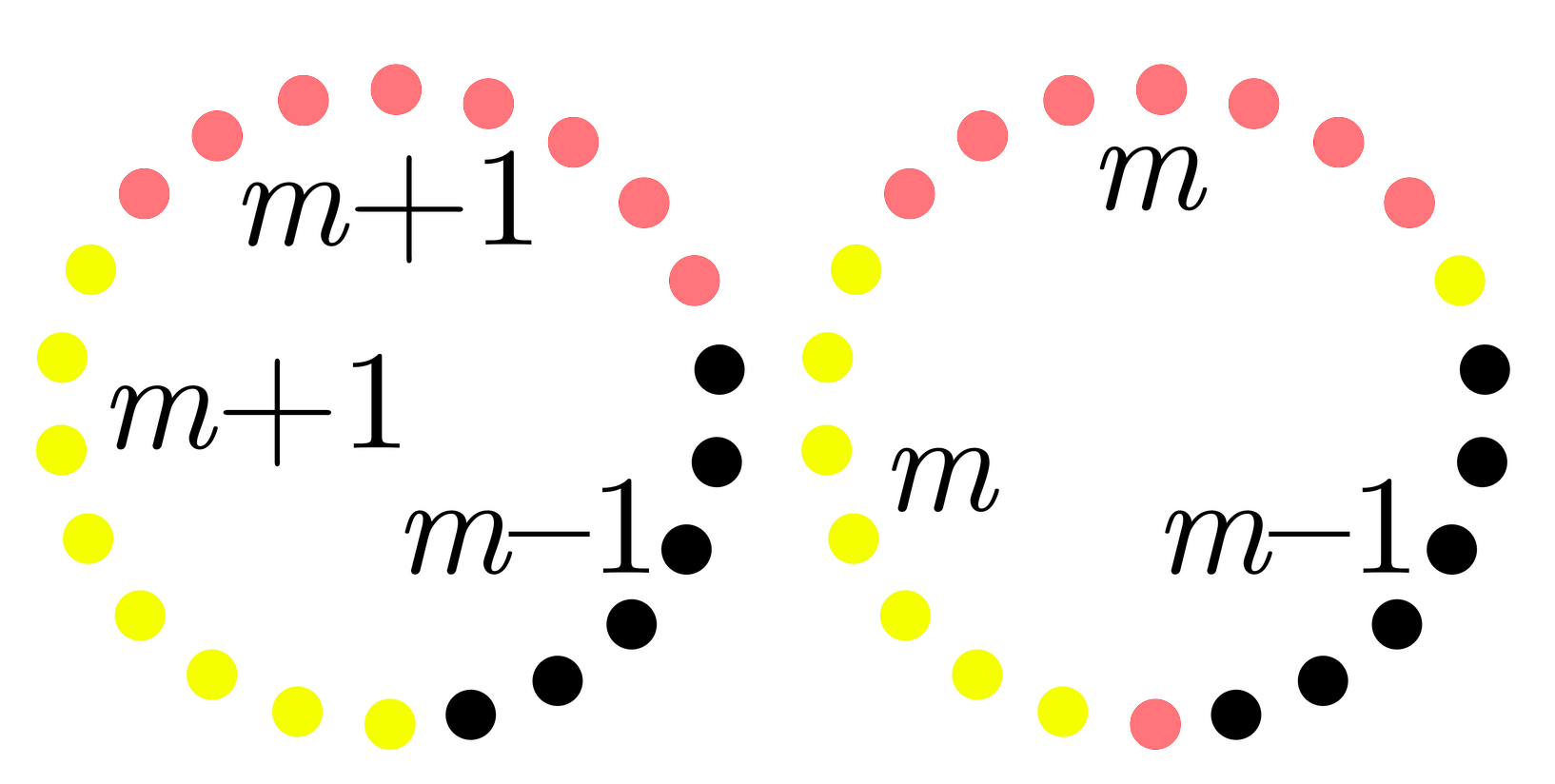 Figure 1
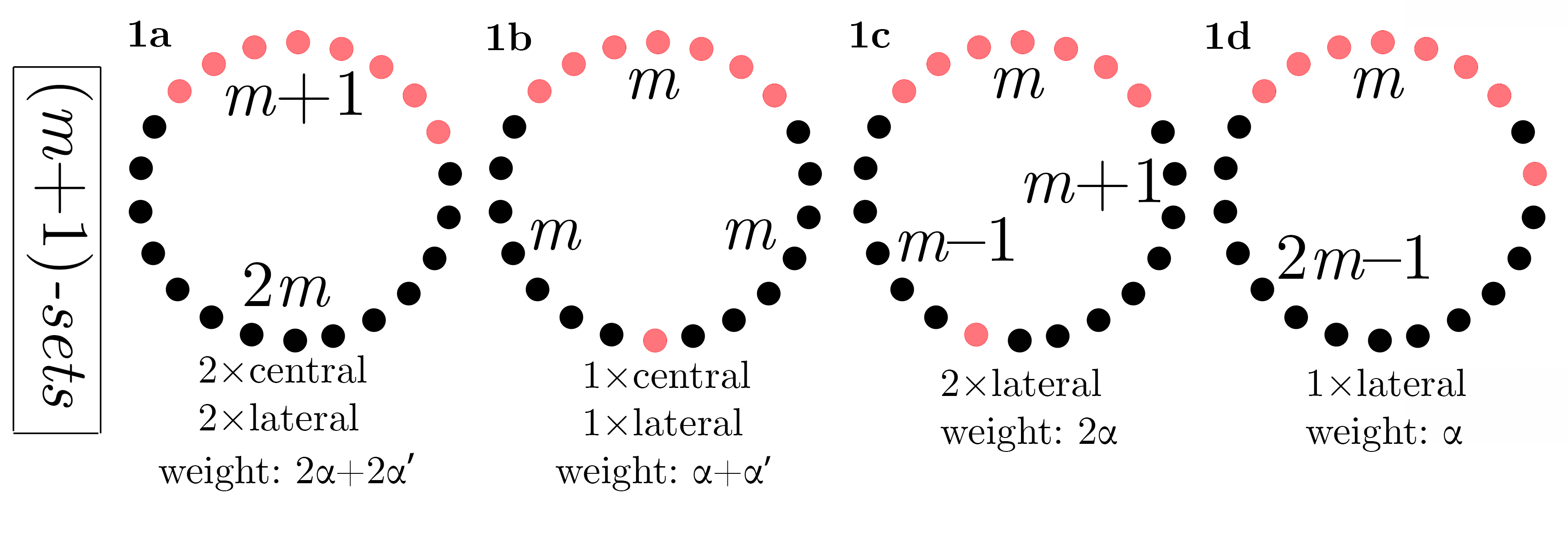 Figure 2
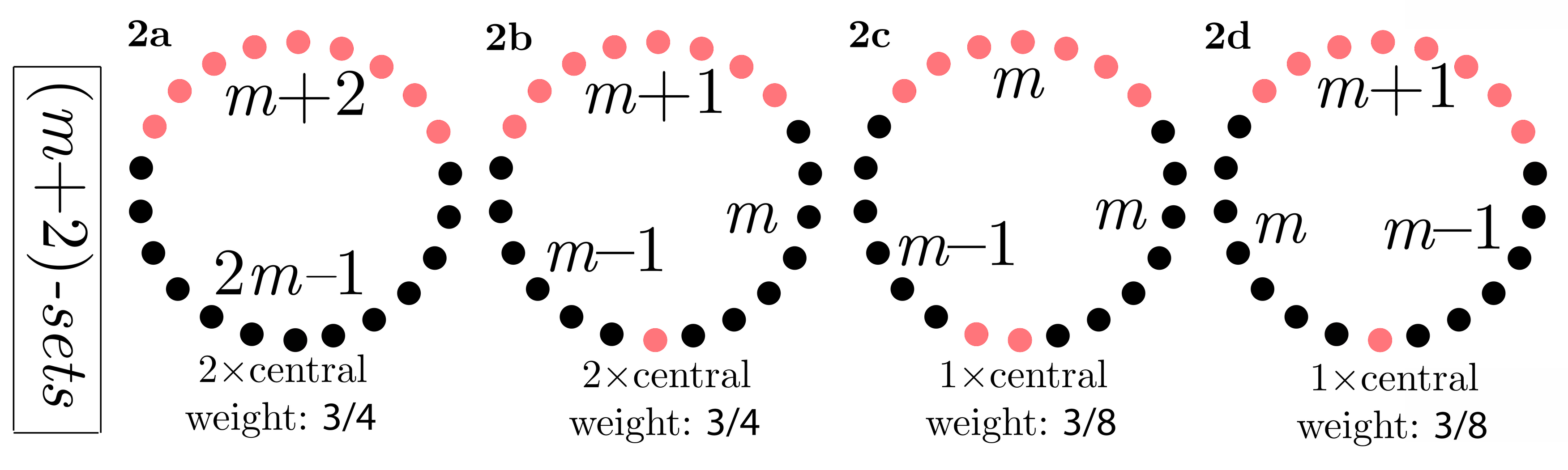 Figure 3
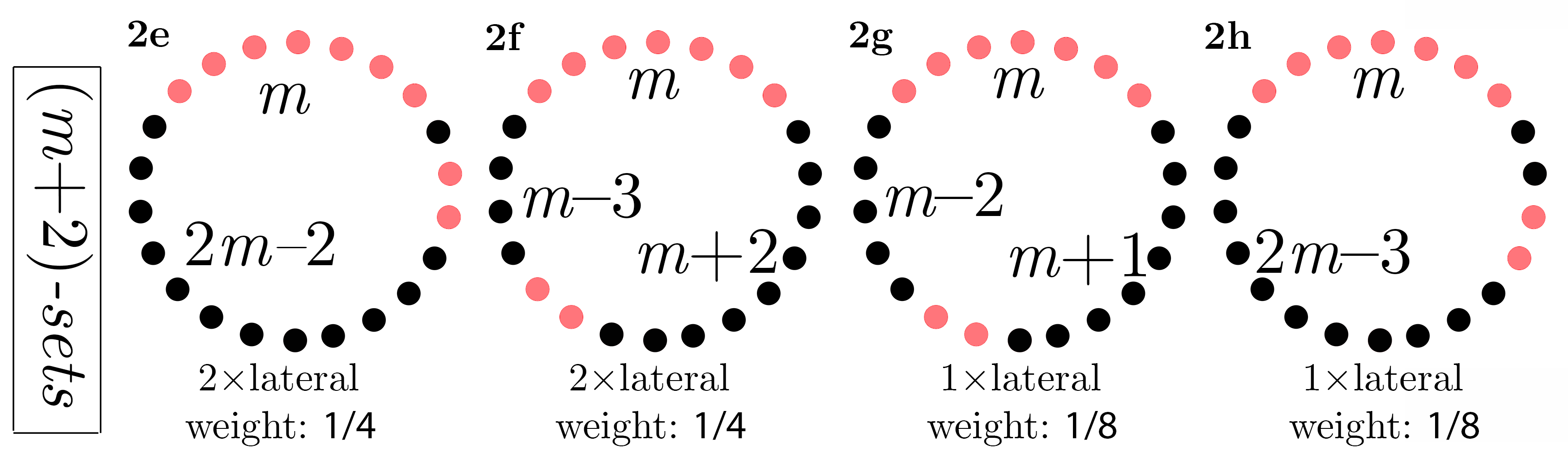 Figure 4
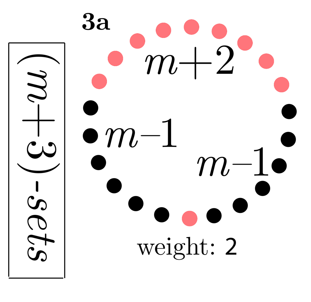 Figure 5
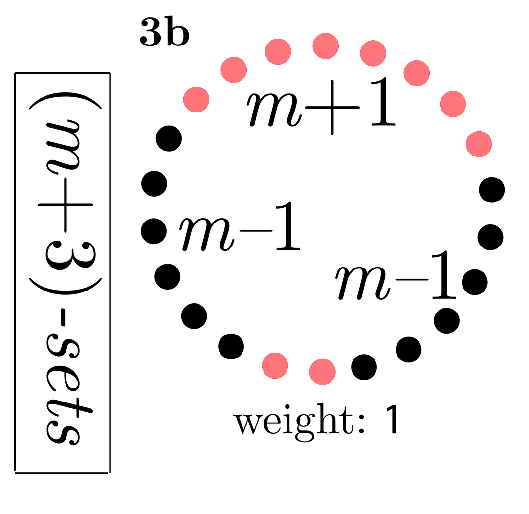 Figure 6
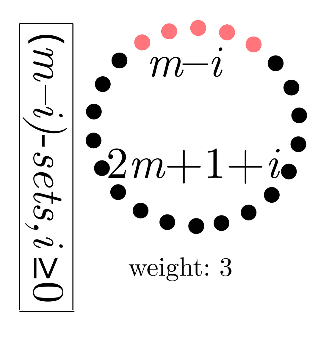 Figure 7
Peer Reviews
No public reviews on file for this paper yet. If you reviewed it on a platform where reviews are public (OpenReview, ICLR, NeurIPS, ICML), you can paste yours below so the community can read it here.
Videos
No videos yet. Explain this paper in a talk, walkthrough, or lecture? Add one.
Families of sets with no matchings of sizes 3 and 4
Peter Frankl, Andrey Kupavskii111Moscow Institute of Physics and Technology, Ecole Polytechnique Fédérale de Lausanne; Email: [email protected] Research supported by the grant RNF 16-11-10014.
Abstract
In this paper, we study the following classical question of extremal set theory: what is the maximum size of a family of subsets of such that no sets from the family are pairwise disjoint? This problem was first posed by Erdős and resolved for by Kleitman in the 60s. Very little progress was made on the problem until recently. The only result was a very lengthy resolution of the case by Quinn, which was written in his PhD thesis and never published in a refereed journal. In this paper, we give another, much shorter proof of Quinn’s result, as well as resolve the case . This complements the results in our recent paper, where, in particular, we answered the question in the case for .
1 Introduction
Let be the standard -element set and its power set. A subset is called a family. For , let denote the family of all -subsets of .
For a family , let denote the maximum number of pairwise disjoint members of . Note that holds unless . The fundamental parameter is called the independence number or matching number.
Denote the size of the largest family with by . The following classical result was obtained by Kleitman. Kleitman’s Theorem ([7]) Let be integers. Then the following holds.
[TABLE]
The value is attained on the family of all sets of size greater than or equal to . The following matching example for (2) was proposed by Kleitman:
[TABLE]
(Note that .) Let us mention that for both bounds (1) and (2) reduce to . This easy statement was proved already by Erdős, Ko and Rado [1].
Although (1) and (2) are beautiful results, for they leave open the cases of For , the only remaining case was solved by Quinn [8]. However, his argument is very lengthy and was never published in a refereed journal. In this paper, we reprove his result, as well as extend it to the case .
Theorem 1**.**
Fix an integer . Then for and we have
[TABLE]
The following -matching-free family shows that “” holds in the equality above for any and .
[TABLE]
Theorem 1 bridges the gap that was left between Quinn’s result and the result of the paper [2], where we verified the same statement for . Contrary to the intuition, the problem gets easier as becomes larger, and thus the proof for is more intricate than that of [2].
The proof is based on a non-trivial averaging technique somewhat in the spirit of Katona’s circle method [6]: we choose a certain configuration of sets, show that the intersection of a family satisfying the conditions of Theorem 1 with each such configuration cannot be too large and then average over all such configurations. However, the configuration is quite complicated, the sets in the configuration actually have weights, and, in order to bound the weighted intersection of the family with each configuration, we use some kind of discharging method.
The method we develop here has proved to be very useful and was already used in several papers. In a recent paper [4], we applied it to completely resolve the following problem studied by Kleitman: what is the maximum cardinality of a family that does not contain two disjoint sets , along with their union ? We refer the reader to the papers [2], [4] for a more detailed introduction to the topic and, in particular, to [2] for the discussion of the case of general . See also [5], where the method we developed was applied.
We note that (1) and (2), along with more general statements, are proved using a simpler version of our technique in [3].
2 Preliminaries
Recall that is called an up-set if for any all sets that contain are also in . Since we aim to upper bound the sizes of families with , we may restrict our attention to the families that are up-sets, which we assume for the rest of the paper.
We are going to use the following inequality in the proofs:
[TABLE]
Indeed, we have for any and , so by the formula for the summation of a geometric progression,
[TABLE]
3 Proof of Theorem 1 for
We first prove the theorem for . Suppose that and put for this section. Consider a family with . Take an arbitrary cyclic permutation (assumed in what follows to be the identity permutation for simplicity) and fix three disjoint -element sets that form arcs in that permutation. This is what we call a triple. For , the -triple is the triple of -sets that do not contain the element . It is clear that there is a one-to-one correspondence between the ’s and the triples. For each triple, we define three groups of sets of sizes and assign them weights. We call this ensemble of sets an -family. Note that the arithmetic operations in the definitions of the sets are performed modulo .
We define three groups of sets, indexed by . In what follows, we define group . The -th -set in the -family has the form . The set of size for has the form . That is, it consists of the last elements of the -set, if seen in the clockwise order. The sets form a full chain. The definition of the sets of size is less straightforward. Each of the -sets in the -th group contains the corresponding -set. The -set
[TABLE]
in group is called central. Note that the extra element it has is the element that was left out by the -sets and so is disjoint of for . The two others
[TABLE]
are called lateral and are disjoint of the corresponding and the remaining -set , where . For each , we define two -element sets: the central set
[TABLE]
and the lateral set
[TABLE]
The former ones are disjoint of and the -set from the remaining -th group, where , while the latter ones are disjoint of . Note that and are disjoint for . Finally, we have one -set in each group:
[TABLE]
It is disjoint of the -sets from the other groups.
Each set in each group gets a weight. We denote by the weight of the -element sets, with possible superscripts depending on whether the set is lateral or central, respectively. Put
[TABLE]
Note that . The weights are as follows ():
[TABLE]
Thus, the total weight of all sets in an -family is . Each set that appears in several -families accumulates all the weight that it was assigned. On Fig. 1, we listed all the types of sets that are assigned non-zero weights, together with the corresponding weights. We recommend the reader to verify Fig. 1, since we shall use the information provided on the figure later in the proof! The elements of the ground set are placed on the circle and the sets are represented modulo rotation. We denote by the family of all sets that got non-zero weight for a given permutation . Note that, for each , we have
[TABLE]
Claim 2**.**
To prove the theorem for , it is sufficient to show that for any we have
[TABLE]
Proof.
For an event , denote by its indicator random variable. Denote the identity permutation. Indeed, if we take a permutation uniformly at random, then, for each , we have
[TABLE]
[TABLE]
[TABLE]
Therefore, (7) implies that
[TABLE]
which implies the statement of the theorem for .∎
Our strategy to prove (7) is as follows. For a set , we define the charge to be equal to if , and to be [math] otherwise. Clearly, . If among the -sets in there are no sets from , as well as there are at most -sets, then we are done since each -set appears in exactly three -families. Otherwise, certain -sets do not appear in . Then we transfer (a part of) the charge of the -sets to the -sets that have zero charge. We show that the total charge transferred to each -set is at most its weight. As a result of this procedure, the -sets will have zero total charge, the -sets will have total charge at most , and each -set will have a charge not greater than its own weight. This will obviously conclude the proof of the theorem.
Next, we design a charging scheme that satisfies the above requirements. For the sets of size at most , we transfer their charge within each -family, assuring that the charge that we transferred to a bigger set in one -family is smaller than the weight that this bigger set got from this -family. See Table 1 for all the triples of pairwise disjoint sets we use in the proof. The reader is welcome to verify that all the triples are actually disjoint.
Stage 1. Transferring charge from the -sets to -sets.
Assume that, for some and , the set is in the family. Choose such that . Then at least one set from each of the two pairs \bigl{(}H_{j_{1}}^{(m+2)}(i,i;x), H_{j_{2}}^{(m+2)}(x,i;x)\bigr{)}, \bigl{(}H_{j_{2}}^{(m+2)}(i,i;x), H_{j_{1}}^{(m+2)}(x,i;x)\bigr{)} is missing from . We transfer of the charge of the subsets , , which is at most , to some two of these missing sets. We again remark that, for each , we transfer only the part of the charge of the sets that they got as the member of the -family. We have
[TABLE]
(We could have put instead of , but it does not matter for the calculations.) Since each -set in the -family may get this charge from each of the two groups to which it does not belong, the total charge transferred in that way is at most . The lateral -sets are not going to get any more charge. As for the central -sets, we have to make sure that they will get not more than additional charge.
We note that the -sets will be discharged together with the corresponding -sets.
Stage 2. Transferring charge from pairs of -sets to -sets.
Due to the fact that is an up-set, from now on we may assume that the charge of any -set is 0. Assume that, for some and , where , both and belong to . Then the set is not in and, consequently, has zero charge. Transfer the charge of the sets and , , to . The charge transferred is at most , which is
[TABLE]
since . The -sets are not going to get any more charge.
Stage 3. Transferring charge from -sets paired with -sets to central -sets.
Assume that, for some and , where , both and belong to . Then the central -set is not in and, consequently, received at most charge within the -family (because of the charge possibly transferred on Stage 1). Transfer the charge of the sets , , to . The charge transferred is at most , which is
[TABLE]
The last inequality is valid for any and is easy to verify by a direct calculation. The right hand side is exactly , and so the total charge of the central -sets is at most in each -family. The -sets are not going to get any more charge.
Stage 4. Transferring charge from single -sets to -sets.
After the above redistribution of charges, for each , there are no -sets and at most one -set and -set with non-zero charges in the -family, moreover, we cannot have an -set and two -sets with non-zero charges in the -family.
Assume that for some and , where , the set belongs to . Then one set from each of the two pairs \bigl{(}H_{j_{1}}^{(m+1)}(x;x), H_{j_{2}}^{(m+1)}(i;x)\bigr{)} and \bigl{(}H_{j_{1}}^{(m+1)}(i;x),H_{j_{2}}^{(m+1)}(x;x)\bigr{)} is missing from . We transfer of the charge of the subsets , , which is at most , to each of these missing sets. We have
[TABLE]
Recall that , and, therefore, , which means that no -set gets more charge than its weight up to this stage.
Stage 5. Transferring charge from pairs of -sets to central -sets.
Denote the number of -sets that have non-zero charge (that is, that are contained in ) by . If , then we are clearly done since each -set appears in exactly three -families.
Assume that . On the one hand, it makes an extra contribution to the left hand side of (7). On the other hand, the number of triples with two -sets belonging to is non-zero. Indeed, if, for , we denote by the number of triples with -sets in the family, then, since each -set participates in three triples, we have . Since , we have . Assume that for some and , where , both and belong to . Then the central -set is not in the family. Moreover, no charge was transferred to it from the -family, since we could not have had two -sets and an -set with non-zero charges at the same time after Stage 3. We transfer charge to from the -sets.
First note that we have transferred charge from the -sets to the central -sets, which results in -sets having total charge of . This is precisely what we needed to have, and we are only left to verify that we did not overcharge the central -sets. Unfortunately, we can run into problems in this situation, so we have to consider two cases. First, assume that . Then the charge on each central set in each -family is at most
[TABLE]
The second inequality holds due to the fact that for the function decreases as grows. Therefore, if , then we are done. Let us verify that this inequality is implied by (5). Adding to the right hand side of the inequality, we get
[TABLE]
[TABLE]
where the last inequality holds for any . Thus, we fulfilled all the requirements on the charging scheme and we are done in the case .
In the case , however, we run into trouble: the inequality may not hold. Recall that . We are still fine if since the calculations in (9) still go through in that case. Thus we only need to examine the case , which we assume until the end of this section. The equation means that there are exactly two triples with two -sets from . This is the only part of the proof when we are not going to compare the amount of charge passed to the -sets to the portion of its weight inside the -family. Instead, we compare the charge to the full weight of the -set.
We have two possible configurations with . One possibility is that we have two -sets from forming an interval of length on the circle, and then the two triples contributing to share the same two -sets. In this case, the central -set that we forbid is the same in both triples, and it is of type 1a (see Fig. 1). Recall that this set has weight . The other possibility is that we have two pairs of -sets, with each pair separated on the two sides by a third -set forming a triple with the pair, and by the element missing from the triple, respectively. In this case, in each of the corresponding two -families we forbid a central -set of type 1b. Each of these two sets (that are clearly different) has weight . In either case, we need to transfer amount of charge from the -sets to some of the -sets. We transfer this weight to the central -set(s), possibly overcharging it.
Assume first that we do not have any -element sets in . Then, in either of the possibilities described above, the central -sets have zero charge before Stage 5. Therefore, we are good if the weight of these (one or two) -sets is greater than the amount of charge we transfer to them from the pairs of -sets. Namely, we are good if
[TABLE]
We have
[TABLE]
where the last inequality holds for . Thus, this case is covered.
Finally, assume that there is at least one -element set . Then, as one can see from Fig. 2, it forbids at least one -set of each of the types 1a and 1b to appear. Denote them by . We have seen two paragraphs above that in either case of the arrangement of the -sets we forbid sets of the same type (either one of type 1a, or two of type 1b). Therefore, at least one of that did not get any charge at Stage 5. We assume that it is a set of type 1b (the other case is easier and is treated similarly). The set appears in two -families and got some charge only at Stage 4. Moreover, got at most charge from each of the two -families. Thus, the charge of after all five stages is at most . This, in turn, means that it has extra capacity of at least . We redistribute some part of the charge from the two -sets (that appeared in the -families with the pairs of -sets from ) to . In order to be able to fulfil the requirements on the charging scheme, we need the total capacity of these -sets to be greater than the charge we transfer. More precisely, it is sufficient if the following inequality holds:
[TABLE]
Note that we replaced the capacity of the (one or two) missing central -set(s) by since the -part of the charge may have been already used up by the -sets at Stage 4. We have verified above (see (10)) that the same inequality holds if one replaces with . One can easily see (cf. (5)) that , so we have . The case is examined in its entirety, and the proof of the theorem in the case is complete.
3.1 The case
In the argument above, we assumed that . However, we want to prove the theorem for , which leaves us with two cases: and . If , then we have , and we have to show that at least four sets, including the empty set, are missing from a family with . If there is at most one singleton in , then we are done. If there are at least two singletons, say, and , then is empty, which gives missing sets. The case is covered.
If then , and we have to show that at least sets are missing from . If there is at least one singleton in , say , then is intersecting, and so, by the Erdős-Ko-Rado theorem, a half of the sets are missing from it. This gives missing sets.
Thus, we may assume that there are no sets of size smaller than in . Now we may slightly modify the proof for the case so that it works for . Namely, among the -sets, we give weights only to the central -sets (the weights on other layers stay the same). Claim 2 stays true in this case. Since we do not have sets of size smaller than , we can go to Stage 5 of the analysis, where we want to show that with the new weights (9) holds for any for :
[TABLE]
The last inequality obviously holds. Thus, for we may terminate the proof right after (9). The proof is complete.
4 Proof of Theorem 1 for
We first prove the theorem for . We put for some throughout this section. The logic of this proof is very similar to that of the proof in the case , and the proof is in a sense even simpler. We present it somewhat more concisely.
We fix an arbitrary permutation of the ground set. For simplicity, we assume that is the identity permutation. Quite predictably, define four groups of sets, indexed by and forming an -family. The four -sets in an -family are disjoint and form an interval of length , leaving two contiguous elements out (thus, the -family is indexed by the last of the two missing elements in the clockwise order). In what follows, we define the -th group. The sets in the -th group of size , form a full chain together with :
[TABLE]
We again have both central and lateral - and -sets. The -sets
[TABLE]
in group are called central. Note that the extra element in both sets is left out by the -sets, and so for both is disjoint of the -set from the -th group, . The three others
[TABLE]
are called lateral and are disjoint of the corresponding and of the -set in the -group, .
For each , we define two lateral -element sets:
[TABLE]
and for each we define one central set:
[TABLE]
The former ones are disjoint of the -set from group and the two -sets from the remaining groups, while the latter one is disjoint of the three -sets from the groups . Finally, we have one -element set for each
[TABLE]
Each set in each group gets a weight. We denote by the weight of the -element sets, with possible superscripts depending on whether the set is lateral or central, respectively. The weights are as follows ():
[TABLE]
It is easy to check that, for each and in each group the weight of -element sets sums up to for fixed , and that is positive.
As before, each set that appears in some -families accumulates all the weight that it was assigned. We denote by the family of all sets that got non-zero weight for a given permutation . Analogously to Claim 2, to prove the theorem in this case, it is sufficient to show that for any we have
[TABLE]
For a set , we define the charge to be equal to if , and otherwise. Clearly, . We again design a scheme for the transfer of (a part of) the charge of the -sets to the -sets that have zero charge. We show that the charge transferred to each -set is at most its weight. As a result of this procedure, the -sets will have zero total charge, the -sets will have total charge , and each -set will have charge not greater than its own weight. This will obviously conclude the proof of the theorem.
Next we design a charging scheme that satisfies the above requirements. For it is sufficient in all cases to redistribute the charge within each -family, assuring that the charge that we transferred to the larger set in one -family is smaller than the weight that this bigger set got from this -family.
Stage 1. Transferring charge from triples of -sets to -sets.
Assume that, for some and , where , the sets for , belong to . Then is missing from , and, consequently, has zero charge. Transfer all the charge of the sets , to the missing -set.
The charge transferred is at most , which is
[TABLE]
where the last inequality holds for any . Note that we apply (4) for in the first inequality above (and in several places below). The -sets are not going to get any more charge.
Stage 2. Transferring charge from pairs of -sets to lateral -sets.
Assume that, for some and , where , both and belong to . Then in each of the four pairs \bigl{(}H_{i_{1}}^{(m+2)}(x^{\prime},j^{\prime};x), H_{i_{2}}^{(m+2)}(x^{\prime\prime},j^{\prime\prime};x)\bigr{)}, where one of the -sets is missing from , and, consequently, has zero charge. Note that all these -sets are lateral. Transfer one quarter of the charge of the sets and , , to each of these missing sets.
The charge transferred to each lateral -set is at most , which is
[TABLE]
where the last inequality holds for any . The lateral -sets are not going to get any more charge.
Stage 3. Transferring charge from single -sets to -sets.
After the above redistribution of charges, we have at most one -set with non-zero charge in each -family.
Assume that for some and , where , the set belongs to and still has non-zero charge. Then one set from each of the six triples \bigl{(}H_{j_{1}}^{(m+1)}(\pi(i);x), H_{j_{2}}^{(m+1)}(\pi(x-1);x),H_{j_{3}}^{(m+1)}(\pi(x);x)\bigr{)}, where is a permutation of the set , is missing from . It is not difficult to see that it means that at least three out of the listed sets are missing from . Note that among the possible missing sets there are both central and lateral -sets.
We transfer of the charge of , , to each of the three missing sets. This is at most which is
[TABLE]
We are not going to transfer any more weight to the lateral -sets.
Stage 4. Transferring charge from pairs and triples of -sets.
At this stage only the sets of size greater than or equal to have non-negative charge. Denote the number of -sets that have non-zero charge (that is, that are contained in ) by . If , then we are clearly done.
Assume that . On the one hand, it makes an extra contribution to the left hand side of (12). On the other hand, the number of quadruples with two or three -sets belonging to is non-zero. Indeed, if we denote by the number of quadruples with -sets in the family, for , then we have . Since , we have
[TABLE]
We proceed as follows.
(i) Triples of -sets. Assume that, for some and , where , the sets belong to for all . Then the central -set is not in the family . Moreover, it has zero charge. We transfer charge to this set. We have for , since this function for decreases as grows. Therefore, we have
[TABLE]
The last inequality holds for .
(ii) Pairs of -sets. Assume that for some and , where , exactly two -sets and from the -family belong to . Then in each of the two pairs of central -sets \bigl{(}H_{i_{1}}^{(m+1)}(x^{\prime};x),H_{i_{2}}^{(m+1)}(x^{\prime\prime};x)\bigr{)} for one of the sets is not in the family. Moreover, each of them has received at most charge within this -family (they could have received charge only in Stage 3). We transfer charge to each of the two missing central sets. We have to verify that the charge transferred is at most . Note that . Therefore, it is enough to verify
[TABLE]
The last inequality holds (with equality) since by (4) we have .
Now we only have to make sure that we have transferred enough charge. Indeed, we have transferred a total amount of charge equal to
[TABLE]
Therefore, the total amount of charge that is left on the -sets is at most , moreover, all sets of size not greater than have zero charge, and none of the sets has the charge that is greater than its weight. The inequality (12) is verified, and the proof of Theorem 1 in the case is complete.
4.1 The case
In the argument above, we assumed that . However, we wang to prove the theorem for , which leaves us with two cases: and . If , then we have , and we have to show that at least sets, including the empty set, are missing from a family with . If there is at most one singleton in , then we are done. If there are at least two singletons, say, and , then is intersecting, and, consequently, at least sets are missing from among the sets from . The case is covered.
If then and we have to show that at least sets are missing from . If there is at least one singleton in , say , then, applying (2) to , we get that at least sets are missing from , which is more than 47.
Thus, we may assume that there are no sets of size smaller than in . Now we may slightly modify the proof for the case so that it works for . Namely, among the - and -sets we give weights only to the central - and -sets (each central -set receives a weight of , each central -set receives a weight of , and the weights on other layers stay the same). Since contains no sets of size smaller than , we may go to part 4 of the analysis, where we have to verify the following analogues of (15) and (14) for :
[TABLE]
Both hold for . The rest of the proof stays the same. The proof is complete.
Acknowledgements. We thank the anonymous referees for their helpful comments on the presentation of the paper.
The reference list from the paper itself. Each links out to its DOI / PubMed record.
- 1[1] P. Erdős, C. Ko, R. Rado, Intersection theorems for systems of finite sets , The Quarterly Journal of Mathematics, 12 (1961) N 1, 313–320.
- 2[2] P. Frankl, A. Kupavskii, Families with no s 𝑠 s pairwise disjoint sets , Journal of the London Math. Soc. 95 (2017), N 3, 875–894.
- 3[3] P. Frankl, A. Kupavskii, Two problems on matchings in set families – in the footsteps of Erdős and Kleitman , accepted at J. Comb. Th. Ser. B, ar Xiv:1607.06126
- 4[4] P. Frankl, A. Kupavskii, Partition-free families of sets , accepted at Proceedings of the London Mathematical Society, ar Xiv:1706.00215
- 5[5] P. Frankl, A. Kupavskii, New inequalities for families without k 𝑘 k pairwise disjoint members , J. Comb. Th. Ser. A 157 (2018), 427-434.
- 6[6] G. Katona, Intersection theorems for systems of finite sets , Acta Math. Acad. Sci. Hung. 15 (1964), 329–337.
- 7[7] D.J. Kleitman, Maximal number of subsets of a finite set no k 𝑘 k of which are pairwise disjoint , Journ. of Comb. Theory 5 (1968), 157–163.
- 8[8] F. Quinn, Ph D Thesis, Massachusetts Institute of Technology (1986).