Achievable Rate Region of the Zero-Forcing Precoder in a 2 X 2 MU-MISO Broadcast VLC Channel with Per-LED Peak Power Constraint and Dimming Control
Amit Agarwal, Saif Khan Mohammed

TL;DR
This paper analyzes the achievable rate region of a 2x2 MU-MISO VLC channel with zero-forcing precoding under power and dimming constraints, proposing a Pareto-optimal boundary and a simplified transceiver architecture.
Contribution
It introduces an analytical characterization of the rate region boundary and a novel transceiver design for VLC with dimming control, enhancing understanding and practical implementation.
Findings
Maximum rate region occurs at half of the peak power.
Achievable rates are sensitive to LED and PD placement.
Coverage zones can be defined with acceptable rate reduction.
Abstract
In this paper, we consider the 2 X 2 multi-user multiple-input-single-output (MU-MISO) broadcast visible light communication (VLC) channel with two light emitting diodes (LEDs) at the transmitter and a single photo diode (PD) at each of the two users. We propose an achievable rate region of the Zero-Forcing (ZF) precoder in this 2 X 2 MU-MISO VLC channel under a per-LED peak and average power constraint, where the average optical power emitted from each LED is fixed for constant lighting, but is controllable (referred to as dimming control in IEEE 802.15.7 standard on VLC). We analytically characterize the proposed rate region boundary and show that it is Pareto-optimal. Further analysis reveals that the largest rate region is achieved when the fixed per-LED average optical power is half of the allowed per-LED peak optical power. We also propose a novel transceiver architecture where…
Click any figure to enlarge with its caption.
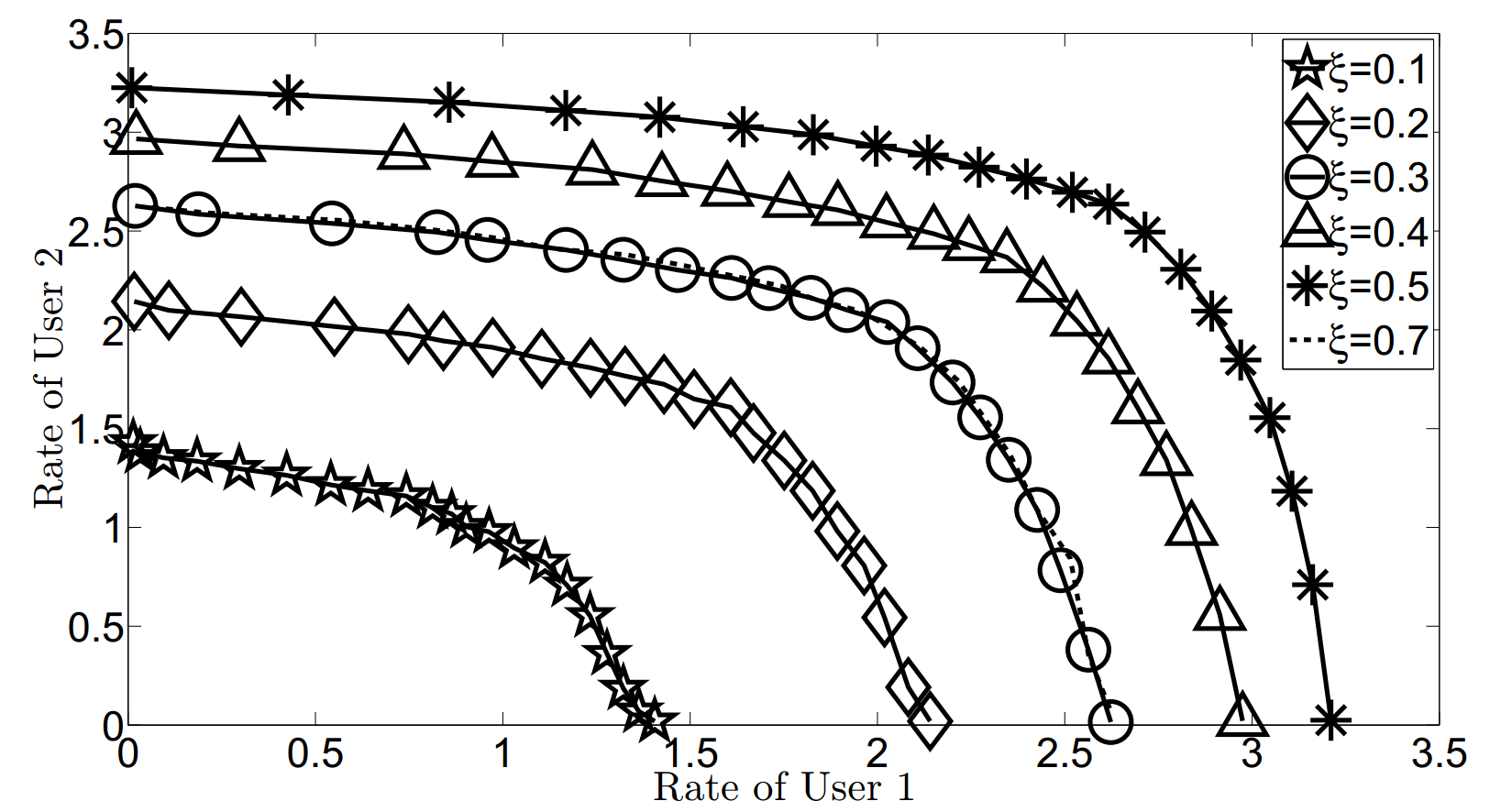 Figure 1
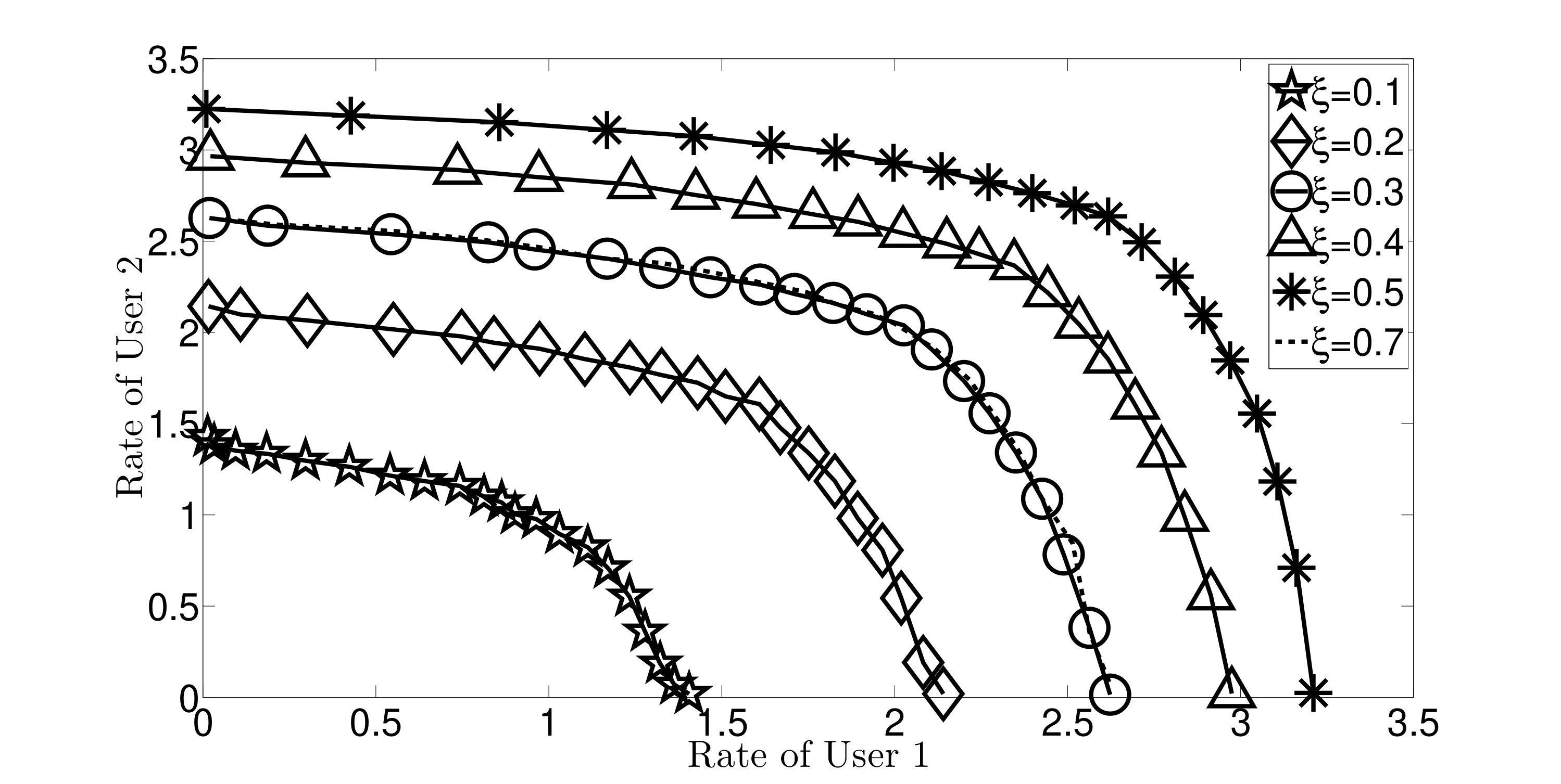 Figure 2
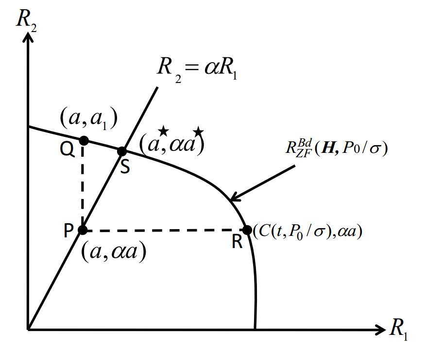 Figure 3
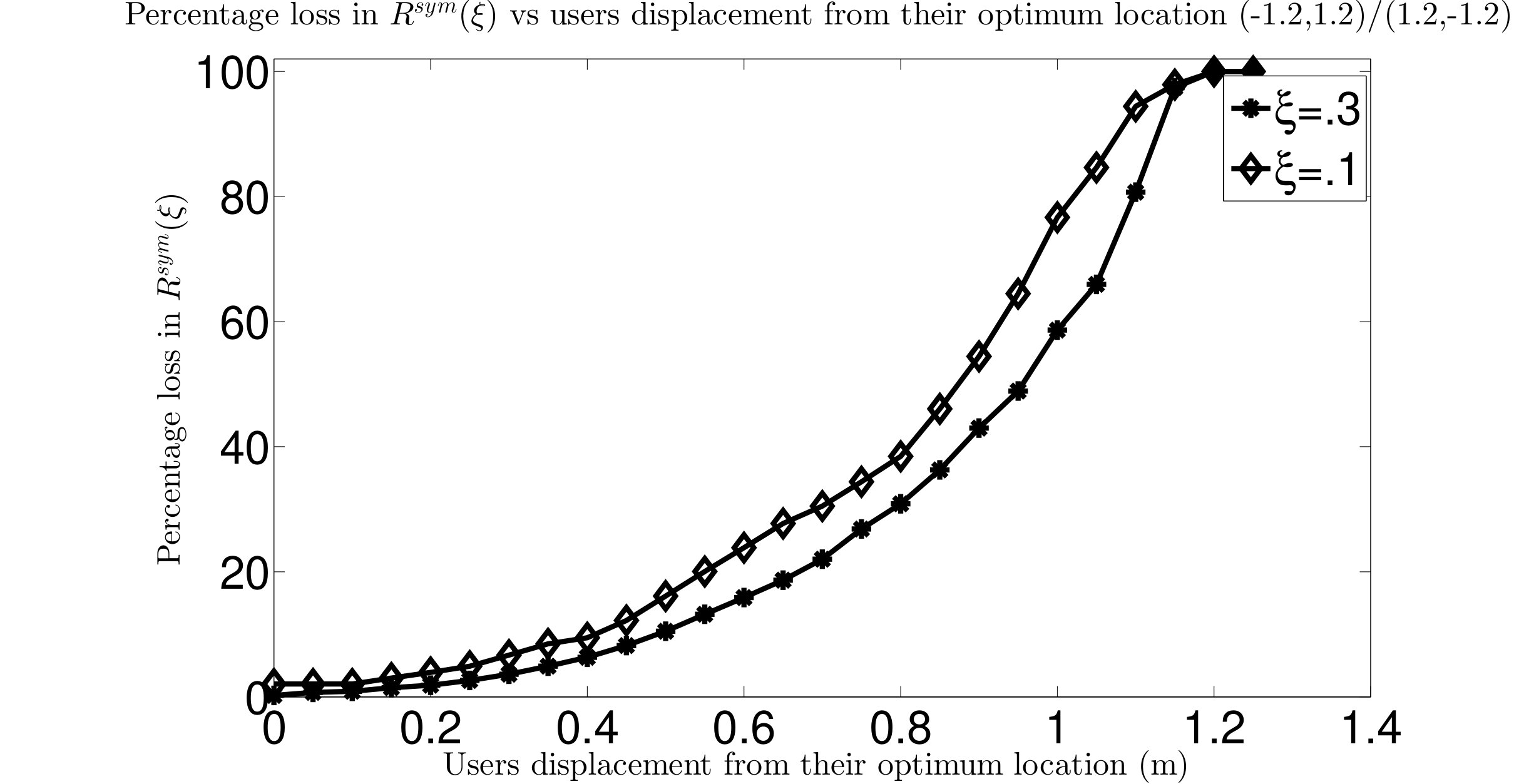 Figure 4
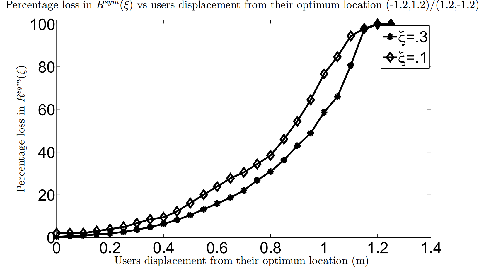 Figure 5
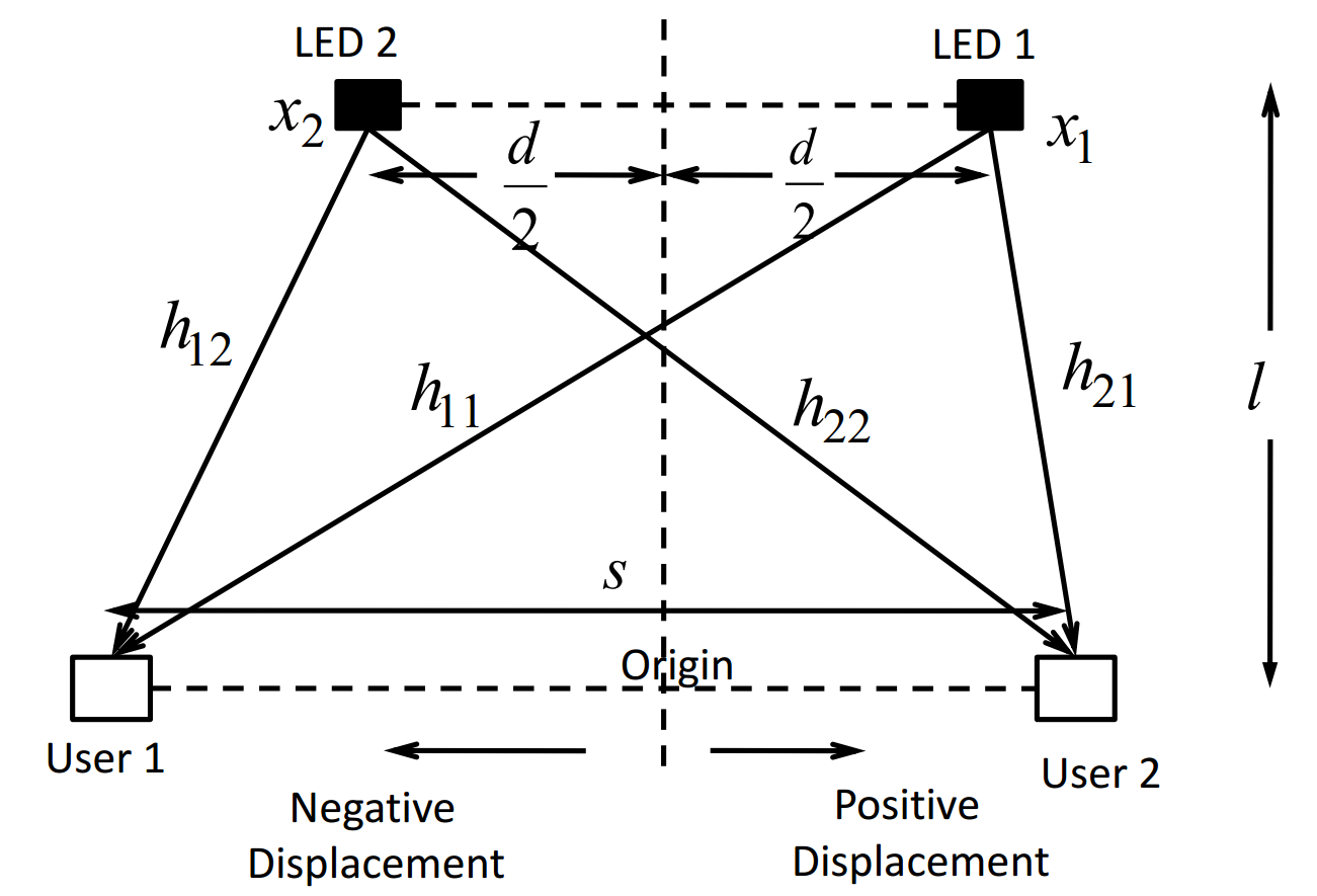 Figure 6
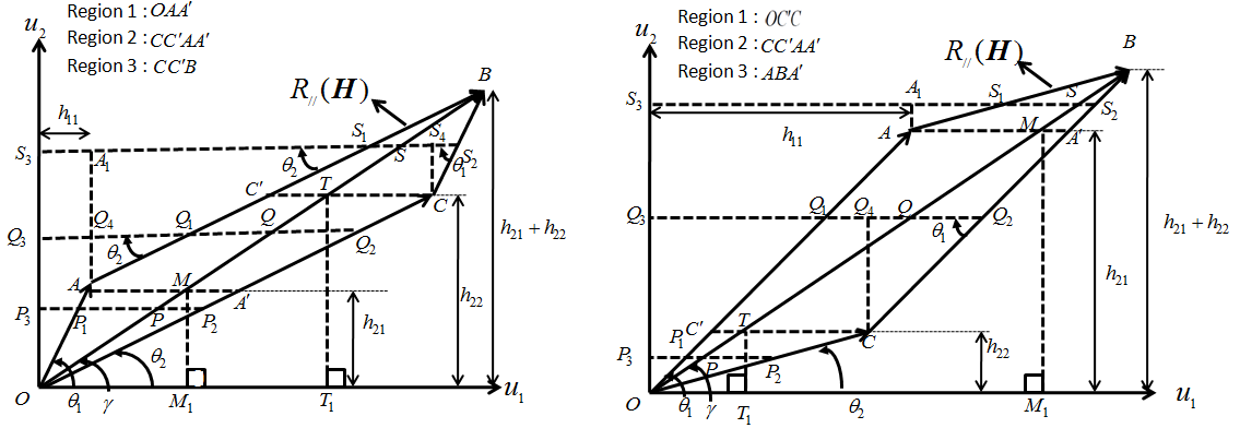 Figure 7
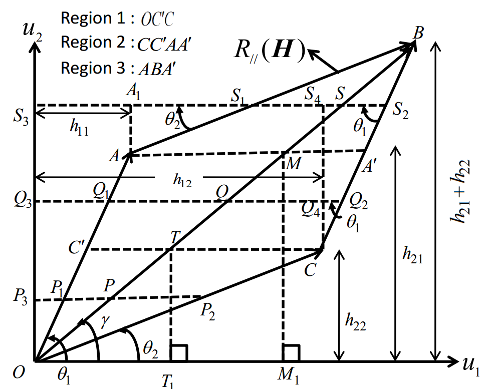 Figure 8
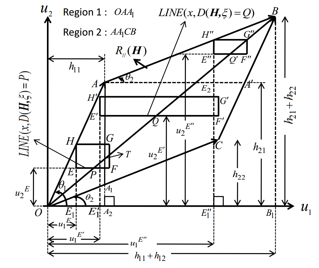 Figure 9
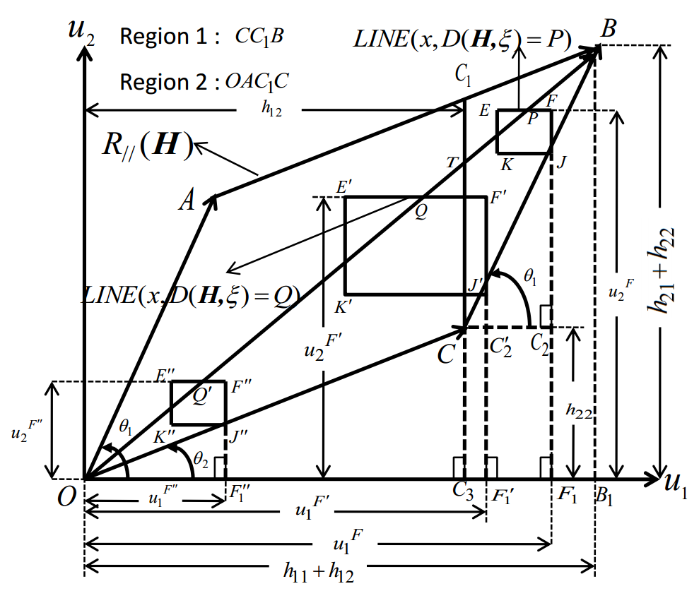 Figure 10
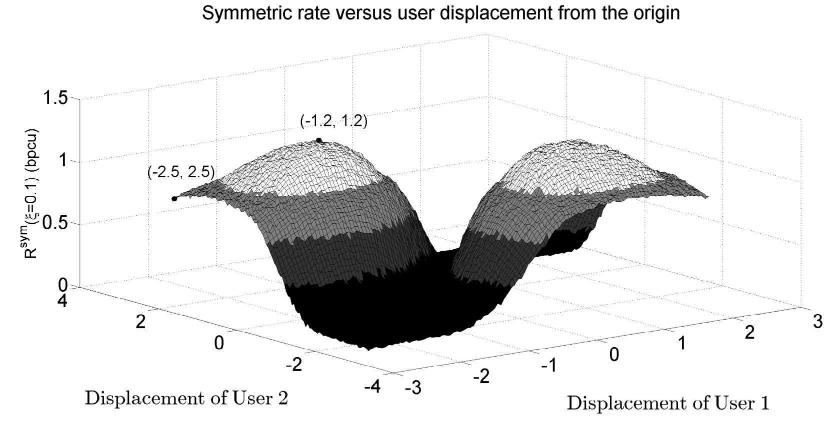 Figure 11
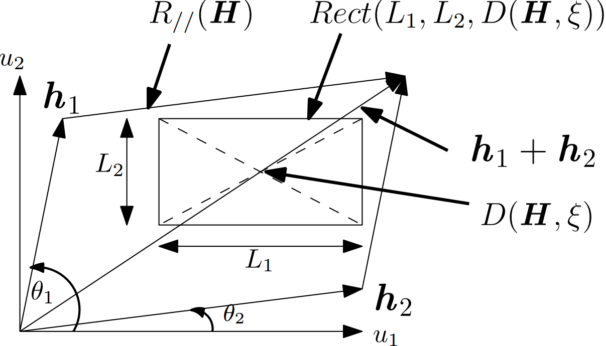 Figure 12
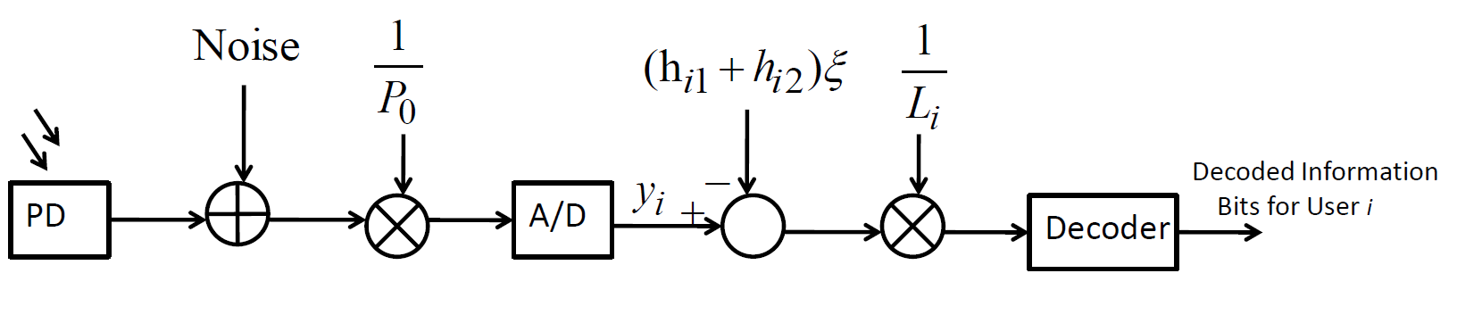 Figure 13
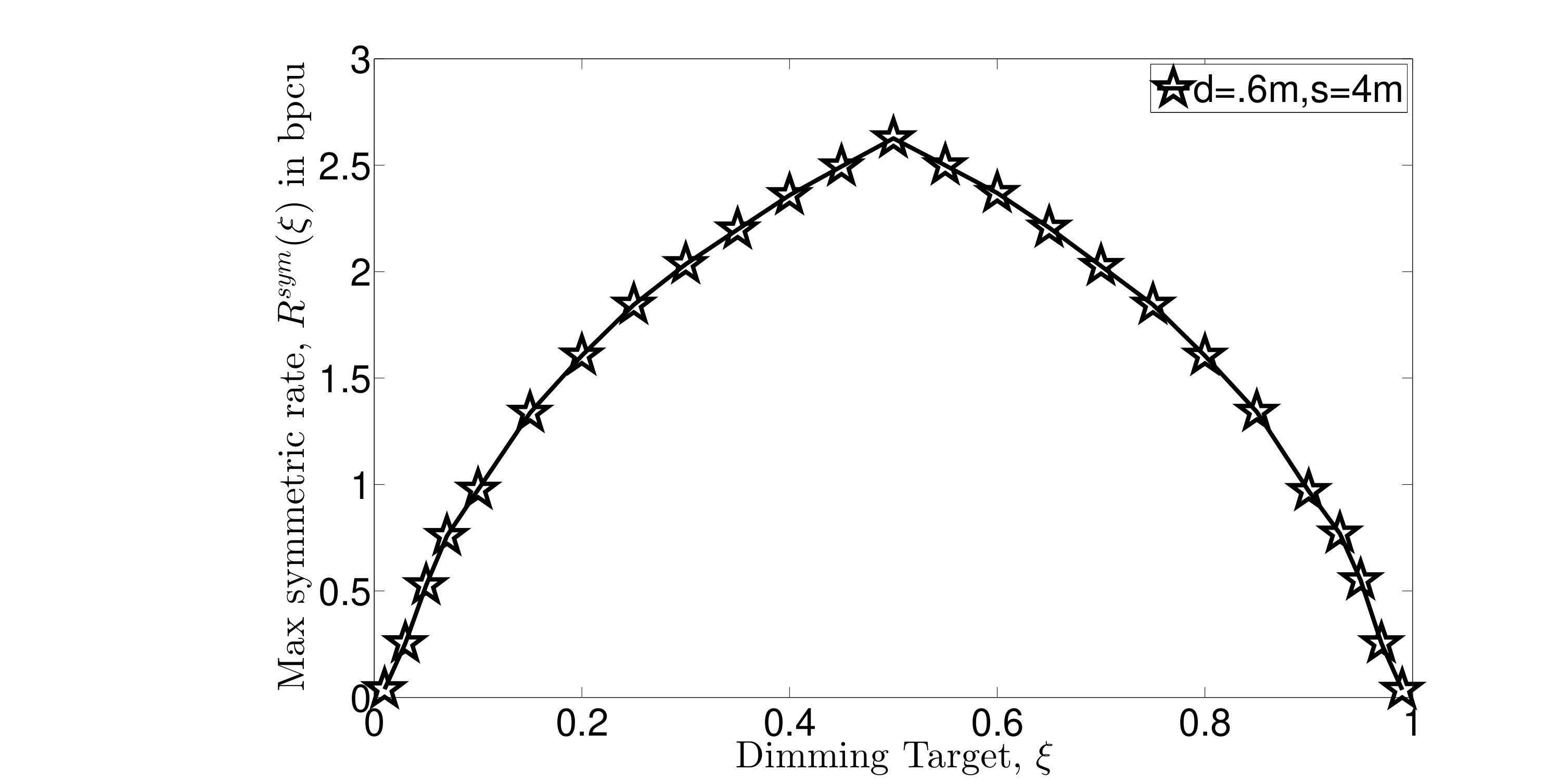 Figure 14
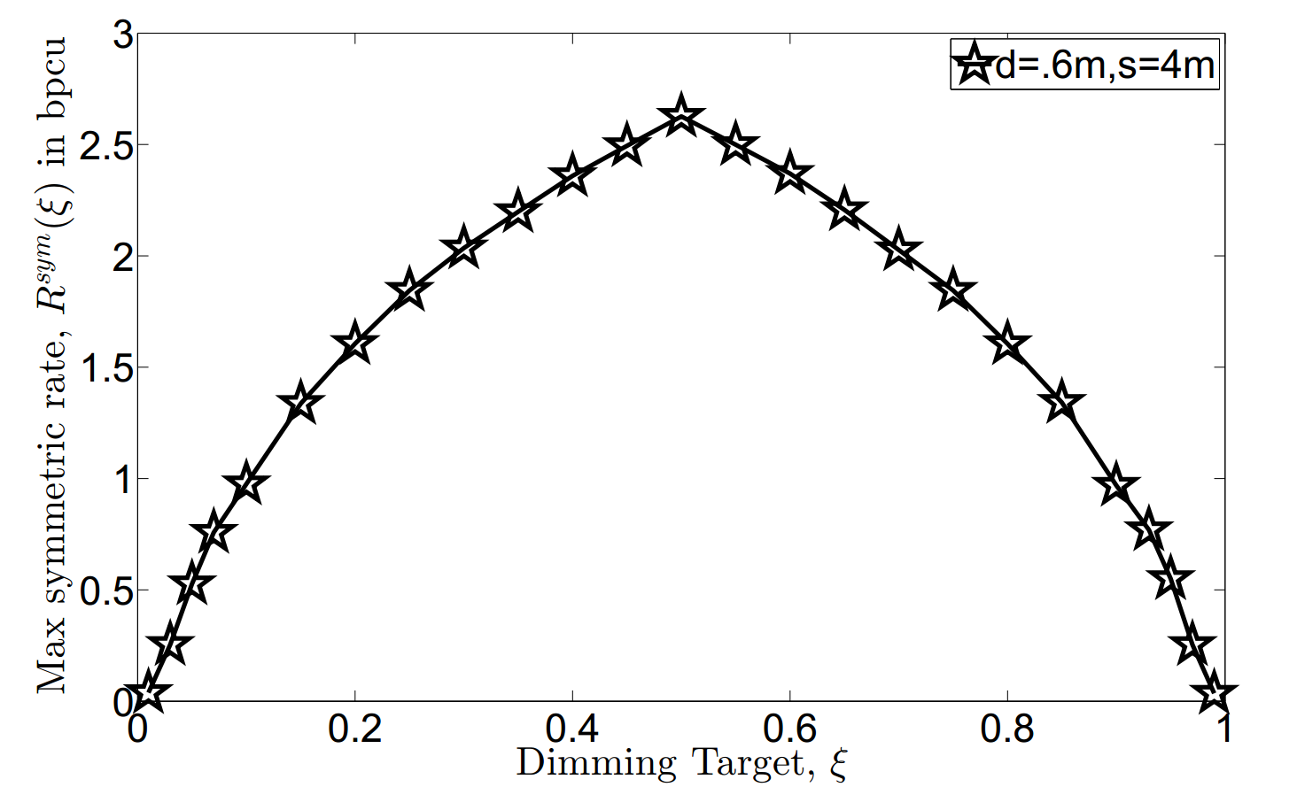 Figure 15
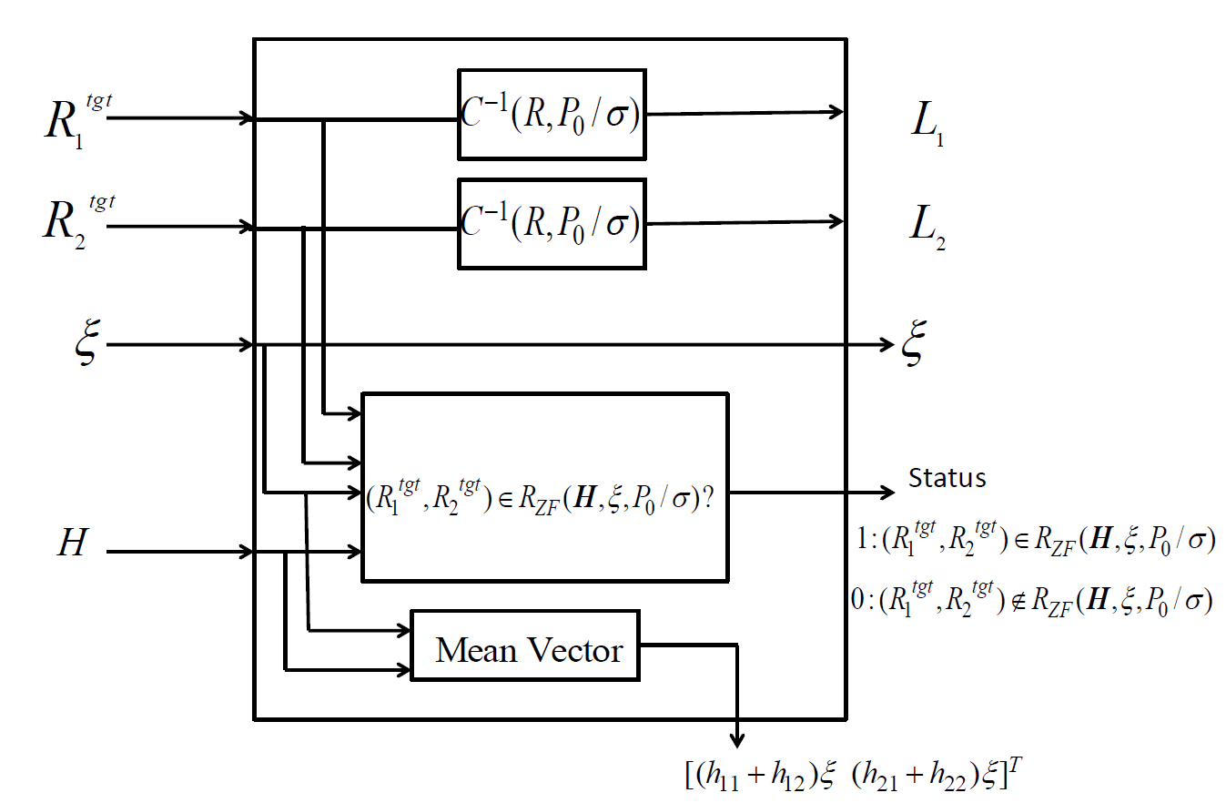 Figure 16
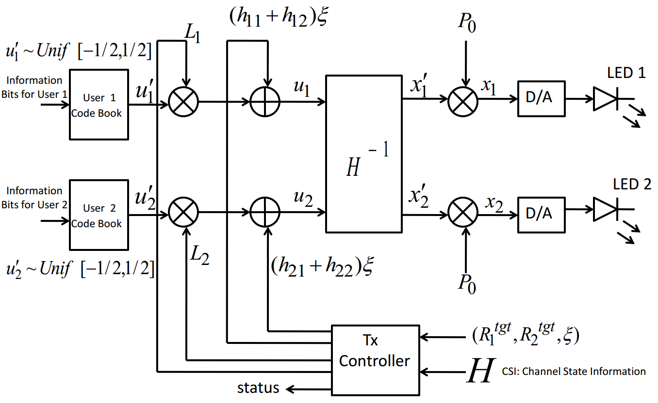 Figure 17
| PD area | 1 |
|---|---|
| Receiver Field of Veiw (FOV) | 60 [deg.] |
| Refractive index of a lens at the PD | 1.5 |
| Semi-angle at half power | 70 [deg.] |
Peer Reviews
No public reviews on file for this paper yet. If you reviewed it on a platform where reviews are public (OpenReview, ICLR, NeurIPS, ICML), you can paste yours below so the community can read it here.
Videos
No videos yet. Explain this paper in a talk, walkthrough, or lecture? Add one.
Achievable Rate Region of the Zero-Forcing Precoder in a 2 2 MU-MISO Broadcast VLC Channel with Per-LED Peak Power Constraint and Dimming Control
Amit Agarwal and Saif Khan Mohammed The authors are with the Department of Electrical Engineering, Indian Institute of Technology Delhi (IITD), New delhi, India. Saif Khan Mohammed is also associated with Bharti School of Telecommunication Technology and Management (BSTTM), IIT Delhi. Email: [email protected]. This work is supported by the Visvesvaraya Young Faculty Research Fellowship (YFRF) of the Ministry of Electronics and Information Technology, Govt. of India.
Abstract
In this paper, we consider the 2 2 multi-user multiple-input-single-output (MU-MISO) broadcast visible light communication (VLC) channel with two light emitting diodes (LEDs) at the transmitter and a single photo diode (PD) at each of the two users. We propose an achievable rate region of the Zero-Forcing (ZF) precoder in this 2 2 MU-MISO VLC channel under a per-LED peak and average power constraint, where the average optical power emitted from each LED is fixed for constant lighting, but is controllable (referred to as dimming control in IEEE 802.15.7 standard on VLC). We analytically characterize the proposed rate region boundary and show that it is Pareto-optimal. Further analysis reveals that the largest rate region is achieved when the fixed per-LED average optical power is half of the allowed per-LED peak optical power. We also propose a novel transceiver architecture where the channel encoder and dimming control are separated which greatly simplifies the complexity of the transceiver. A case study of an indoor VLC channel with the proposed transceiver reveals that the achievable information rates are sensitive to the placement of the LEDs and the PDs. An interesting observation is that for a given placement of LEDs in a 5 m 5 m 3 m room, even with a substantial displacement of the users from their optimum placement, reduction in the achievable rates is not significant. This observation could therefore be used to define “coverage zones” within a room where the reduction in the information rates to the two users is within an acceptable tolerance limit.
Index Terms:
Visible light communication, rate region, zero-forcing, multi-user, multiple-input-multiple-output.
I Introduction
Visible light communication (VLC) is a form of optical wireless communication (OWC) technology which can provide high speed indoor wireless data transmission using existing infrastructure for lighting. One distinctive advantage of VLC technology is that it utilizes the unused visible band of the electromagnetic spectrum and does not interfere with the existing radio frequency (RF) communication in the UHF (Ultra High Frequency) band [1],[2].
In VLC systems, it is common to use intensity modulation (IM) via light emitting diode (LEDs) for transmission of information signal and direct detection (DD) via photodiodes (PDs) for the recovery of the information signal [1]. Contrary to RF systems, in VLC systems the modulation symbols must be non-negative and real valued as information is communicated by modulating the power/intensity of the light emitted by the optical source (LED). The modulation symbols are also constrained to be less than a pre-determined value as the intensity of the light emitted by the LED is peak constrained due to safety regulations and also due to the limited linear range of the transfer function of LEDs [1],[3]. Moreover, due to constant lighting the mean value of the modulation symbol is also fixed (i.e., non-time varying) and can be adjusted according to the users’ requirement (dimming target) [4], [5].
Due to these constraints, analysis performed for RF systems is not directly applicable to VLC systems. For example, the capacity of the RF single-input-single-output (SISO) additive white Gaussian noise (AWGN) channel is well known and it has been shown that the Gaussian input distribution is capacity achieving. For the case of the optical wireless AWGN SISO channel with IM/DD transceiver, closed form expression for the capacity is still not known, though several inner and outer bounds have been proposed [6, 7, 8]. However, it has been shown that the capacity achieving input distribution for the IM/DD SISO AWGN optical wireless channel is discrete [9], and has been computed numerically in [10]. Similarly, for the case of dimmable VLC IM/DD SISO channel with peak constraint, there is no closed from expression for the capacity. However following a similar approach as in [6], an upper and lower bound is presented in [11].
Recently, there has been a lot of interest in multi-user multiple-input multiple-output/single-output (MU-MIMO/MISO) VLC systems, where multiple LEDs are used for information transmission to multiple non-cooperative PDs (users) [12],[1]. Such systems have been shown to enhance the system sum rate when compared to SISO VLC systems [13],[14] .
In [13], the information sum rate of MU-MIMO VLC broadcast systems has been studied under the non-negativity constraint on the signal transmitted from each LED, and also a per-LED average transmitted power constraint with no dimming control. The block diagonalization precoder in [13] is used to suppress the multi-user interference and the numerically computed achievable sum rate is shown to be sensitive to the placement of the users and the rotation of the PDs. However, they do not consider peak power constraints which is important due to eye safety regulations and also due to the requirement of limited interference to other VLC systems.
Per-LED peak and average power constraint has been considered in [14], where the sum-rate of the zero forcing (ZF) precoder is maximized in a IM/DD based MU-MIMO/MISO VLC systems. However, in many practical scenarios fairness is required and therefore maximizing the sum rate might not always be the desired operating regime. For example we would like to find the maximum possible rate such that each user gets the same rate. Such operating points can only be obtained from the rate region characterization of the MU-MIMO VLC systems. In [15], authors have proposed inner and outer bounds on the capacity region of a two user IM/DD broadcast VLC system where the transmitter has a single LED and each user has a single PD. Per-LED average and peak power constraints are considered. The authors have extended their work to more than two users in [16]. However, in both [15] and [16], the transmitter has only one LED. Furthermore, dimming control is not considered in [13, 14, 15, 16].
The capacity/achievable rate region of a IM/DD based VLC broadcast channel where the transmitter has LEDs and users having one PD each, is still an open and challenging problem, primarily due to the non-negativity, peak and average constraints on the electrical signal input to each LED.
In this paper, we consider the smallest instance of this open problem along with dimming control, i.e., with LEDs at the transmitter and users (each having one PD). Dimming control is required in indoor VLC systems since the illumination should not vary with time on its own and should be controllable by the users. Therefore, in this paper, in addition to the peak and non-negativity constraints, we constrain the average optical power radiated by each LED to be fixed, i.e., non-time varying. Subsequently in this paper we refer to this system as the MU-MISO VLC broadcast system.
The major contributions of this paper are as follows:
In Section III, we propose an achievable rate region for the MU-MISO VLC broadcast system with the ZF precoder. In this section through analysis we show that the per-LED non-negativity and peak constraint restricts the information symbol vector for the two users (i.e., to lie within a parallelogram . Each achievable rate pair then corresponds to a rectangle which lies within . The rate to the user depends on the length of the rectangle along the -axis. Due to the same average optical power constraint at each LED, these rectangles should also have their midpoint (i.e., point of intersection of the diagonals of the rectangle) at a fixed point on the diagonal of denoted by D.111Out of the two diagonals of , we refer to the one which has one end point at the origin = (0,0). This fixed point D on the diagonal of is non-time varying, but can be controlled by the user depending upon the illumination requirement. This feature of the proposed system enables dimming control. 2. 2.
In Section III, We also mathematically define the proposed rate region of the ZF precoder for a fix dimming target. 3. 3.
In Section IV, we analytically characterize the boundary of the proposed rate region by deriving explicit expressions for the largest possible length along the -axis of some rectangle inside whose midpoint coincides with the fixed point D on the diagonal of and whose length along the -axis is given. Through analysis we also show that the rate region boundary is Pareto-optimal. 4. 4.
We also analyze the variation in the rate region with change in the dimming level. In depth analysis reveals that the largest rate region is achieved when the fixed point D lies at the midpoint of the diagonal of , i.e., when the fixed per-LED average optical transmit power is half of the per-LED peak optical power. 5. 5.
For practical scenarios with fairness constraints, through analysis we show that the largest achievable rate pair such that is given by the unique intersection of the proposed rate region boundary with the straight line . 6. 6.
In Section V, from the point of view of practical implementation we also propose a novel transceiver architecture where the same channel encoder can be used irrespective of the level of dimming control. 7. 7.
Analytical results have been supported with numerical simulations in Section VI. It is observed that for a fixed placement of the two LEDs, the achievable information rates are a function of the placement of the two PDs/users. Specifically, we observe that for a given placement of the two LEDs, there exists an optimal placement of the two users which maximizes the symmetric rate. Another interesting observation is that in a 5 m 5 m 3 m (height) room with the two LEDs attached to the ceiling and the two PDs placed in the horizontal plane at a height of 50 cm above the floor, even a user displacement of 60 cm from the optimal placement results in only approx. a 10 percent reduction in the symmetric rate when compared to the symmetric rate with the optimal placement of PDs222For this study the dimming control is such that the average optical power radiated from each LED is 30 percent of the peak allowed optical power. This allows for substantial mobility of the user terminals around their optimal placement which is specially desirable when the user terminals are mobile/portable. A practical application of the results derived in this paper could be in defining coverage zones for the PDs/users, i.e., the maximum allowable displacement of the users for a fixed desired upper limit on the percentage loss in the achievable information rates.
II System Model
We consider a IM/DD MU-MISO VLC broadcast system. The transmitter of the MISO system is equipped with two LEDs and each user has a single photo-diode (PD) (see Fig. 1).333 Since each of the two users has a single PD we will be interchangeably using user and PD in subsequent discussions. The LED converts the information carrying electrical signal to an intensity modulated optical signal and the PD at each user converts the received optical signal to electrical signal. The transmitter performs beamforming of the information symbols towards the two non-cooperative users. Let and be the information symbols intended for the first and second user respectively, where and are the information symbol alphabets for user 1 and user 2 respectively. Let be the optical power transmitted from the LED (). At any time instance, the transmitted optical power vector is given by
[TABLE]
where and is the beamforming matrix. In this paper, we consider the following power constraints for our dimmable VLC system.
The instantaneous power transmitted from each LED is non negative and is less than some maximum limit due to skin and eye safety regulations [3]. Further, such a maximum limit on the transmitted power is required also due to limited interference requirement to the neighboring VLC systems, i.e.
[TABLE]
Since our VLC system is dimmable we further impose a per-LED average power constraint of the type
[TABLE]
where is the dimming target [5]. For the sake of analysis, we define as the normalized power transmitted from each LED. Consequently, the normalized optical power transmitted from each LED must satisfy the following constraints given by
[TABLE]
Assuming , to be the normalized received electrical signal at the user (after scaling down by ), the normalized received signal vector is given by444In subsequent discussions, by “received electrical signal”, we refer to the “normalized received electrical signal”.
[TABLE]
[TABLE]
where is the channel gain matrix. The channel gain coefficients between the LED and the user is denoted by 555Note that ’s are non negative and model the overall gains of the line of sight (LOS) optical path between the LED and the user and also the responsivity of the PD of the user [3]. We further define and to be the channel vectors from LED 1 and LED 2 respectively. Further, and are the sum of the thermal noise and ambient light-induced shot noise at the respective users666Note that the above noise impairments of the received signal are the main impairments that are commonly assumed in VLC systems [3]. and are independent of and [12]. The noise signals are i.i.d. zero mean real AWGN with variance , where is the variance of the noise before the scaling down of the received signal by , i.e.,
III An achievable rate region of the channel in (5)
In this section, we derive an achievable rate region for the channel in (5) using the ZF precoder. For the MU-MISO system discussed in section II, the ZF precoding matrix is uniquely given by , i.e., . Thus the received signal vector is given by
[TABLE]
i.e., there is no multi-user interference (MUI). Since
[TABLE]
and (see (4)) it follows that, the information signal vector must be limited to the region
[TABLE]
The region is a parallelogram with its two non parallel sides as and (see in Fig. 2). In addition to this, the diagonal of the parallelogram is the vector as shown in Fig. 2.
Let be the mean information symbol vector. From (7) and (4), the mean information symbol vector is given by
[TABLE]
where step (a) follows from (5). Therefore, the mean information symbol pair is a point corresponding to the tip of the vector . From (8) it is clear that the vector is a diagonal of (see Fig. 2). For a given , the tip of the mean information symbol vector is therefore a fixed point on the diagonal . We denote this point by
[TABLE]
With the ZF precoder, the broadcast channel in (5) is reduced to two parallel SISO (single-input single-output) optical channels between the transmitter and the two users (see (6)). Since and are independent and originate from different codebooks, it follows that . From (8), we know that must belong to the parallelogram and therefore
[TABLE]
In general we choose and to be intervals of the type [9]. Let the length of the intervals and be and respectively, i.e. . With and as intervals, it is clear that must be a rectangle whose length along the axis is and that along the axis is . In this paper we assume and , to be uniformly distributed in the interval and respectively.777At high SNR (), uniformly distributed information symbol is near capacity achieving [10]. Therefore, for a given and , the mean information symbol pair will lie at the point of intersection of the two diagonal of the rectangle . We will subsequently call this point of intersection as the “midpoint” of the rectangle and will denote it by .
From (III), it follows that the mean information symbol pair must exactly coincide with , i.e.
[TABLE]
The ZF precoder transforms the broadcast channel into two parallel SISO channels Let and denote the information rates achieved on these SISO channels with distributed uniformly in . Any given and satisfying the conditions in (11) and (12) would satisfy the optical power constraints in (4) and would therefore correspond to an achievable rate pair for the broadcast channel in (5). Since a rectangle in the plane corresponds to a unique and and vice versa, it follows that any rectangle lying inside the parallelogram and having its midpoint at will correspond to an achievable rate pair. In this paper, for the broadcast channel in (5), we therefore propose an achievable rate region which consists of rate pairs corresponding to such rectangles (one such rectangle is shown in Fig. 2). We define our proposed rate region more precisely in the following. Towards this end, we first formally define the achievable rate of a SISO AWGN optical channel, where the transmitted information symbol is constrained to lie in an interval.
Result 1**.**
[From [6], [10]] The achievable information rate of a SISO channel (where and depends on the interval only through its length , and is given by the function
[TABLE]
here denote the uniform distribution in the interval and is the mutual information between and .
Result 2**.**
[From [6], [10]] The function is continuous with respect to and increases monotonically with increasing for a fixed .
Let denote the unique rectangle having its midpoint as and whose length along the axis is and that along the axis is (see Fig. 2). Any such rectangle will correspond to an achievable rate pair given by
[TABLE]
For a given the proposed achievable rate region for the ZF precoder is given by
[TABLE]
where .
IV Characterizing the Boundary of the Rate Region
In this section, we completely characterize the boundary of the rate region, , for a fixed . Towards this end, for each information rate achievable by the first user, we find the corresponding maximum possible information rate achievable by the second user.* Each pair of and its corresponding maximum possible is therefore a point on the boundary of the proposed rate region*. By increasing from [math] to its maximum possible value, all such pairs characterize the boundary of the rate region.
From (15), we know that any achievable rate pair in the proposed rate region corresponds to some rectangle . The rate to the user, i.e. depends only on the length of this rectangle along the -axis. Since the function is monotonic and continuous in its first argument, each value of corresponds to a unique and vice versa. Therefore, towards characterizing the boundary of , we note that for a given ,i.e., for a given length along the -axis, we would like to find the largest possible ,i.e., the largest possible such that the rectangle lies entirely inside . Hence, we can characterize the boundary of simply by varying from [math] to its maximum possible value (denoted by ), and for each value of we find the largest possible which gives us a corresponding rate pair on the boundary of the rate region .
For a given () the corresponding information rate pair lies on the boundary of the proposed rate region . We denote this information rate pair by . From (14), this information rate pair is given by
[TABLE]
[TABLE]
This then completely characterizes the boundary of the rate region , which is given by888 From (16) and (17) it is clear that the exact computation of and requires the computation of for which we derive closed form expressions in the next section. Computation of and also requires us to compute the function which is done numerically.
[TABLE]
It is noted that the analysis done in this paper is applicable to any placement of the users and the LEDs. Subsequently, we follow the following convention that, by LED 1 we shall refer to the LED whose channel vector has a higher inclination angle (from the axis) than the inclination angle of the channel vector of the other LED.
Let the inclination of the vector and from the axis be and respectively (see Fig. 2). From our definition of LED 1 and LED 2 (see the above paragraph), it follows that . Therefore it follows that . Since
[TABLE]
Hence, implies that
[TABLE]
In the following proposition, we first compute the maximum value of and subsequently we derive the maximum value of for each value of .
Proposition 1**.**
The largest possible value of (i.e., length of the interval ) such that there exists a rectangle which lies completely inside the parallelogram , is given by
[TABLE]
Proof.
See Appendix A. ∎
It is clear from (1) in Proposition 1 that is a continuous function of and .
Remark 1**.**
The function is a continuous function of and is symmetric about , i.e.
[TABLE]
From (1) it is clear that since (see (IV)) is linearly increasing for and is linearly decreasing for . Hence has a unique maximum at .
Remark 2**.**
The function has its unique maximum at , i.e.
[TABLE]
Proposition 2**.**
For a given , the largest possible such that there exists a rectangle , is given by
[TABLE]
*where is given by
Case I: *
[TABLE]
Case II:
[TABLE]
*where .
is given by
Case I: *
[TABLE]
*where
Case II: *
[TABLE]
Proof.
See Appendix B. ∎
Lemma 1**.**
The function is a monotonically decreasing and continuous function of .
Proof.
From Proposition 2 it is clear that for a given both and are continuous and monotonically decreasing function of . From this it follows that is a continuous and decreases monotonically with increasing . ∎
Lemma 2**.**
The proposed rate region boundary is Pareto-optimal. That is, for any two rate pairs and on the boundary , if then it must be true that and if then it must be true that .
Proof.
Let and be any two rate pairs on the boundary such that . Then from ((16) and (17)) it follows that there exists and such that and , , where the functions is defined in (13). From Result (2), we know that for a given , is a continuous and monotonically increasing function of its first argument. Since , it follows that . From Lemma 1, we know that is a monotonically decreasing function of , and therefore , and hence . Similarly, it can also be shown that, if then it must be true that . This completes the proof. ∎
Lemma 3**.**
For a given and , the function is symmetric about , i.e.
[TABLE]
Proof.
See Appendix C. ∎
Using Lemma 3 along with the definition of the rate region boundary in (IV) we get the following result.
Result 3**.**
The proposed rate region boundary is symmetric about , i.e.
[TABLE]
The following theorem shows that for , the largest rate region is achieved when .
Theorem 1**.**
For a fixed ,
[TABLE]
Proof.
See Appendix D. ∎
The proposed rate region boundary can be used to compute many practical operating points. Consider a case where we are interested in finding the largest achievable rate pair such that . This operating point could make sense, if for example the average data throughput requested by user 2 is times that of the throughput requested by user 1.
Moreover, for a given and , the maximum achievable rate pair of the form is given by where is defined as
[TABLE]
Theorem 2**.**
* is unique and lies on the boundary .*
Proof.
See Appendix E. ∎
Remark 3**.**
From the proof in Appendix E it is clear that Theorem 2 is non-trivial as it depends on the monotonicity and continuity of , which is shown in Lemma 1. If Lemma 1 were not true, Theorem 2 would not hold.
Result 4**.**
Using Theorem 2 and (38) of Result 3 it follows that for a given , is symmetric about , i.e.
[TABLE]
Corollary 2.1**.**
From the geometrical interpretation of Theorem 2 it follows that lies on the intersection of the straight line and the rate region boundary . Further, from the Pareto-optimality of the proposed rate region boundary, it follows that there is only a unique point of intersection between the line and .
IV-A Maximum symmetric rate
Note that for the special case of is nothing but the maximum achievable symmetric rate which we shall denote by
[TABLE]
From Theorem 2 it is clear that the maximum symmetric rate is nothing but the largest rate such that the rate pair lies on the boundary . From the characterization of the boundary points in (IV), it follows that there must exist for some such that
[TABLE]
and therefore
[TABLE]
since from Result 2 we know that is a continuous and monotonic function. From 14 it follows that there exists a rectangle corresponding to the rate pair where satisfies 44.
Since it follows that this rectangle is infact a square. Further, from the definition of in (2) it follows that this is the largest sized square whose midpoint is at and has side length .
Hence, the maximum achievable symmetric rate corresponds to the largest sized square which is completely inside and has its midpoint at
V A Novel Transceiver Architecture
In this section we propose a novel transceiver architecture for the practical implementation of the proposed MU-MISO VLC system to achieve any rate pair (see Section IV), under a per-LED peak power constraint of and a controllable dimming target.
In Fig. 3, we have shown the block diagram of both the transmitter and the receiver. The block diagram in Fig. 3(a) depicts the transmitter, the block diagram in Fig. 3(b) depicts the controller for the transmitter which we call as Tx controller and the block diagram in Fig. 3(c) depicts the receiver. The working of this transceiver is as follows.
Consider a scenario where the rate requested by User 1 and User 2 are bpcu and bpcu respectively and to satisfy the lighting requirement inside the room the required dimming target is . We call this rate pair , as the target rate pair of the system. The Tx controller first checks if this target rate pair lies in the proposed achievable rate region (see Section IV). If the target rate pair lies inside the proposed achievable rate region, (i.e., ) then the Tx controller flags , otherwise it flags [math] (see status output of the Tx controller in Fig. 3(b)). If this flag is 1, then the Tx controller provides and , the lengths of the intervals and . From (15) we know that since there must exist some such that and . From Result 2 we also know that for a given , is a monotonic function of , and therefore there exists a corresponding inverse function such that and . It then follows see Fig. 3(c). In the Tx controller we also have a block which outputs the mean information symbol vector (defined in (9)).
Further, in Fig. 3(a) the information bits for user 1 and user 2 are coded separately using independent codebooks each having i.i.d. codeword symbols which are unifromly distributed in . The codeword symbols for user 1 and user 2 are denoted by and respectively (note that and are the information symbols for User 1 and User 2 respectively). From Section III, we know that the information symbols for the user must be uniformly distributed in the interval i.e., (since the horizontal length of the rectangle corresponding to the rate pair is , the vertical length of this rectangle is and its midpoint is ). Therefore, starting with the codeword symbol we can get the information symbol by
[TABLE]
This is also shown in Fig. 3. The information vector is then precoded with and scaled by to give the transmit signal vector . It is noted that the proposed transmitter architecture in Fig. 3(a) allows us to use the same channel encoder/codebook irrespective of the dimming target . This is because the effect of the dimming control is only in shifting the mean of the information symbols (see the adders in Fig 3(a)).999Note that different target rates can be achieved by the same codebook through puncturing of the codewords.
At the receiver after performing the operations shown in Fig. 3(c), we obtain the received vector as given by (5).
VI Numerical Results and Discussions
In this section, we present numerical results in support of the results reported in previous sections. For all numerical results we consider an indoor office room environment where the room is m m and its height is 3 m. The two LEDs are attached to the ceiling and the two PDs (users) are placed at a height of 50 cm from the floor of the room. The two LEDs and the PDs lie in a plane perpendicular to the floor of the plane. The LEDs are placed 60 cm apart and the ratio is fixed to 70 dB. The channel gains are modeled for an indoor line of sight (LOS) channel. The other parameters used for simulation are given in Table I. All these parameters and the channel model are taken from prior work [3, 17, 18, 14].
In Fig. 4, for a LED separation of 0.6 m and PD (user) separation of 4 m such that the placement of both the LEDs and the PDs is symmetric101010Both the line segment joining the two users and the line segment joining the two LEDs have the same perpendicular bisector., we plot the proposed rate region boundary (see IV), for
For a given , it is observed that the boundary is indeed Pareto-optimal as is stated in Lemma 2. We also observe that as increases from to , the rate region expands and then it shrinks with further increase in from onwards to . We have also observed that rate region boundary is same for both and as is stated in Result 3 (see the dotted line and the solid line marked with circle in Fig. 4). It is also observed that gives us the largest rate region as is stated in Theorem 1. The expansion/shrinking of the rate region with changing is explained in the following.
For a given , the points on the rate region boundary correspond to rectangles in the plane having their midpoints at , i.e., on the diagonal and at a distance of from the origin. As increases, the midpoint of the rectangles move away from the origin and towards the interior of the parallelogram . This allows us to fit bigger rectangles and hence the rate region expands. As is increased beyond the midpoint of the rectangles moves towards the other end of the diagonal and hence the size of the rectangles reduces thereby shrinking the rate region.
In Fig. 5, for a fixed user separation of m, an LED separation of cm and symmetric placement of LEDs and PDs, we plot the maximum achievable symmetric rate as a function of varying . We numerically find this operating point by considering all possible points in the - plane which lie in the achievable rate region and also lie on the line . Then among all these possible points we choose the one which has the largest component along the axis. From the figure it is observed that the variation in the maximum symmetric rate with change in the dimming target is small when is around , as compared to when is small. For example, when is reduced from to (i.e., reduction), the corresponding maximum symmetric rate drops only by . However when is reduced by from to , the maximum symmetric rate decreases by approximately . From this it appears that the maximum symmetric rate is lesser sensitive to variations in the dimming target around as compared to variations around smaller values of . It is also observed that symmetric rate is symmetric about as is stated in Result 4 (symmetric rate is nothing but for ).
We next study the variation in the maximum symmetric rate when the two users (PDs) are moved along a line parallel to the ceiling (at a height of 50 cm above the floor) while the two LEDs are stationary and fixed to the ceiling with a fixed separation of 60 cm between them and the dimming target is also fixed to . Further, the two LEDs and the two PDs are co-planar. In Fig. 6, we plot the symmetric rate on the vertical axis as a function of the displacement111111Displacement is nothing but the distance of the user from the origin (see Fig. 1. of the two users from the origin (origin is the point of intersection of the perpendicular bisector of the line joining the LEDs with the line joining the two users, see Fig . 1). In Fig. 6 a positive displacement implies that the user PD is located on the right side of the origin and vice versa (see Fig. 1).
It is observed that the maximum symmetric rate is almost zero if the displacement of both the users is same, i.e., the two users are almost co-located. In the figure this is represented by the dark black region. This is expected since in that case the channels to the users is also the same and hence the performance of the ZF precoder degrades. From the figure we observe that starting with both the users at the origin, as user 2 moves towards the right and User 1 moves towards left the maximum symmetric rate increases sharply (in the figure the colour changes from dark black to light black to gray to white as the displacement vector moves from to ). This happens because as the users move away from each other, their channels become distinct i.e., the angles between the vectors and increases and hence the area of increases. This results in an increase in the largest sized square that can be fit into with center at . This then implies that the maximum symmetric rate would also increase (see the discussion in Section IV-A for the correspondence between the largest square and the maximum symmetric rate). With further increase in the separation between the two users the angular separation between the channel vectors does not increase as sharply as before. At the same time, due to increased path loss from the LEDs to the users, the area of starts decreasing which results in the decrease in the maximum symmetric rate. This can be seen in the figure, as the colour changes back from white to gray, as we move from the displacement vector to . This shows that the maximum symmetric rate is dependent on the location of the users and therefore there is an optimal location121212By the optimum user location we mean the displacement vector of the users at which we get maximum . for both the users which results in the highest symmetric rate. In Fig. 6 the optimum location is , or .
Next in Fig. 7, for a fixed LED separation of 60 cm we plot the percentage loss in the maximum symmetric rate (w.r.t. the symmetric rate at the optimum location) with the users’ displacement from their optimum location for two different values of .
It is observed that the percentage loss increases with increasing displacement of the PDs from their optimal location. Further, the increase in the percentage loss is small when the displacement is small as compared to when the displacement is large. For example, with , the percentage loss increases only by as the displacement increases from 0 cm to 40 cm. However with a further increase in displacement from 40 cm to 80 cm, the percentage loss increases sharply from to . A similar behavior is also observed with , though for a given displacement the loss is greater when as compared to when . A practical application of this study could be in defining coverage zones for the PDs, i.e., the maximum allowable displacement for a fixed desired upper limit on the percentage loss. For example, in the current setup with , for a upper limit on the percentage loss, the maximum allowable displacement is roughly 70 cm. It therefore appears that indoor VLC systems allow for a lot of flexibility in the movement of the user terminals without significant loss in the information rate.
VII Conclusion
We have proposed an achievable rate region for the MU-MISO broadcast VLC channel under per-LED peak power constraint and dimming control. The boundary of the proposed rate region has been analytically characterized. We propose a novel transceiver architecture to implement such systems. Interestingly, the design of encoder/codebook is independent of the dimming target, which reduces the complexity of the transceiver. Work done in this paper reveals that, in an indoor setting, the two users have enough mobility around their optimal placement without sacrificing their information rates. Our work can also be applied to a 2-D setting, where the users are allowed to move in a plane rather than being restricted to a line.
Appendix A Proof of Proposition 1
Proof.
Under the condition in (IV), to find we need to consider three scenarios that cover all geometrically possible parallelograms : (a) ( and ; (b) ; and (c) and .
For a given dimming target, , let denote the length of the longest line segment parallel to the -axis lying completely inside and whose midpoint coincides with the point ( is defined in (III)). For any rectangle , its side along the axis is a line segment inside . From the definition of , it follows that for any rectangle . Additionally, the longest line segment of length corresponds to a rectangle . Hence, it is clear that , i.e.
[TABLE]
In the following, we firstly evaluate the expression for for scenario (a), i.e., when the channel gains satisfy ( and . Towards this end, we partition into three regions, Region as is shown in Fig. 8. We now derive an expression for depending upon the region where lies. In Fig. 8 we denote by the point if lies in Region 1, by the point if lies in Region 2 and by the point if lies in Region 3. Next, we compute when lies in .
**Computation of when : ** The point belongs to Region 1 if and only if
[TABLE]
where the point denote point of intersection of the diagonal and . Further, the line is the line parallel to the -axis. Next, by looking at the right angle triangle in Fig. 8, it follows that , where denotes inclination of the diagonal, , of the parallelogram from the -axis. Since, from Fig. 8, , and , it follows that
[TABLE]
Since the point is nothing but the point , from (III), it follows that . Using and (48) in (47) we have that if and only if
[TABLE]
For all such values of the dimming target, , satisfying (49), it follows that Next, we evaluate when .
Since is the length of the line segment parallel to the -axis having its midpoint at point and lying completely inside . it follows that
[TABLE]
where both the line segments and are parallel to the -axis. Further, lies on the line whereas lies on the line as shown in Fig. 8. Next, we evaluate and . To this end, from Fig. 8, we compute the length of the line segment as follows
[TABLE]
where step (a) follows from the fact that, is equal to the co-ordinate of the point along the -axis and therefore from (III), we have . In step (a) we have also used the fact that since is a right angle triangle having . Hence, it follows that . Step (b) also follows from two facts. Firstly, is equal to the co-ordinate of the point along the -axis and therefore from (III), we have that and secondly, from (19), we know that . Similarly from Fig. 8, we calculate the length of as follows
[TABLE]
where step (a) follows from the fact that, is equal to the co-ordinate of the point along the -axis and therefore from (III), we have that . In step (a) we have also used the fact that is a right angle triangle having . Hence, it follows that . Step (b) follows from two facts. Firstly, is equal to the co-ordinate of the point along the -axis and therefore from (III), we have that and secondly, .
Using (A) and (A) in (50) we see that when (since in scenario (a)), we have
[TABLE]
**Computation of when : ** Point lies in Region 2= if and only if
[TABLE]
where is the point of intersection of the line segment and the diagonal (see Fig. 8). In the following we firstly show that if and only if
[TABLE]
Towards this end, we firstly derive an expression for . From the right angle triangle in Fig. 8, we know that and since , . We have
[TABLE]
Since the point is nothing but the point , from (III), we have and from (48), it follows that . In (54), we substitute by , by the R.H.S in (56) and by to get
[TABLE]
For all such values of the dimming target, , satisfying (A), it follows that Next, we evaluate when . For this scenario, from Fig. 8 we see that
[TABLE]
where construction of and is similar to the construction of and (see Fig. 8), except the fact that lies on instead of . Next, we evaluate and . To this end, using the similar steps as for the evaluation of (see (A)) we have,
[TABLE]
However, evaluation of is not the same as evaluation of , as the point lies on the line segment whereas the point lies on the line . Towards this end, using Fig. 8, we evaluate as follows
[TABLE]
[TABLE]
Using (59) and (A) in (58), we see that when , i.e. (since in scenario (a)), we have
[TABLE]
[TABLE]
where step (a) follows from the fact that , since for scenario (a), we know that
Computation of when :
Point lies in Region 3= if and only if . Using (56) and the fact that (from (III)), we have
[TABLE]
Next, we evaluate when . From Fig. 8 it is clear that when then is given by
[TABLE]
where and are the intersections of the straight line parallel to the axis passing through , with the line segment and respectively. Next, we evaluate and . To this end, using similar steps as for the evaluation of (see (A)) we have,
[TABLE]
However, evaluation of is not same as evaluation of , as the point lies on the line segment whereas the point lies on the line . Towards the evaluation of , using Fig. 8, we have
[TABLE]
Using (A) and (A) in (64), we see that when , i.e. (since in scenario (a)), we have
[TABLE]
where step (a) follows from the fact that , since for scenario (a), we know that
Therefore for the scenario (a), we have the expression of as follows
[TABLE]
Since
[TABLE]
and
[TABLE]
where the above two inequalities follows from the simple mathematical manipulations, and therefore the expression in (73) can be further simplified. To this end, we consider two cases based on the values of .
Case (a):
For this case we know that and hence
[TABLE]
Since from (74) and (75), we know that and and hence, for from (73) and (76) we have
[TABLE]
Case (b):
For this case we know that and hence
[TABLE]
Since from (74) and (75), we know that and and hence, for from (73) and (78) we have
[TABLE]
Therefore from (77) and (79) the final expression of for scenario (a) is as follows
[TABLE]
Using similar arguments as for scenario (a), we evaluate for Scenario (b): ; and for Scenario (c): and as follows.
To this end, we first partition into three regions as shown in Fig. 9. Next, we denote by the point if lies in Region 1, by the point if lies in Region 2 and by the point if lies in Region 3.
Using (56) and (48) we can also show that the point lies in if and only if , lies in iff and it lies in iff Next, we evaluate when lies in Region .
Following similar steps as for scenario (a), from Fig. 9 it follows that when , i.e., when
[TABLE]
Similarly, using Fig. 9 it can be shown that when , i.e., when
[TABLE]
Further, using Fig. 9 it can be shown that when , i.e., when
[TABLE]
Following the steps used to arrive at (82) from (73) in scenario(a), for scenario (b) and (c) also we get the same final expression for as in (82). This completes the proof. ∎
Appendix B Proof of Proposition 2
Proof.
Similar to proposition 1, for proving proposition 2, we consider three mutually exclusive scenarios. (a) and ; (b) ; and (c) and . Moreover, from the definition of LED 1 and LED 2, it follows that, the channel matrix satisfies (IV), i.e. For a fixed , in the following, for a given , we derive the expression for the maximum , (i.e., length of the side of the rectangle along the -axis (vertical length)), such that there exists a rectangle , i.e.
[TABLE]
To this end, for a fixed ,131313Once we fix , location of the point gets fixed (see (III)). and given , we construct all such possible rectangles and among them we choose the rectangle having the maximum possible vertical length.
To get this rectangle we first construct a horizontal line segment of the length parallel to the -axis such that its midpoint coincides with the point . We denote this line segment by , i.e.
[TABLE]
where and Since , from the definition of it follows that lies completely inside .
Given any horizontal line segment of length parallel to the -axis, any rectangle inside having this line segment as one of its side can be constructed in two possible ways, either by extending it vertically downwards or extending it vertically upwards.141414By extending a horizontal line segment vertically downwards/upwards, we mean that we create a rectangle by drawing two vertical lines from the end points of this horizontal line segment in the downward/upward direction and then connecting the other two end points of these two vertical lines to form a rectangle. Subsequently, we shall refer to these construction methods as “downward extension” and “upward extension”.
Using this for a given we can construct a rectangle by extending the line segment vertically upwards. We denote this rectangle by
[TABLE]
where . Let denote the largest possible vertical length of all such rectangles which lie completely inside and are constructed by the upward extension of the line segment , i.e.
[TABLE]
Similarly, we construct any rectangle of vertical length by extending the line segment vertically downwards. We denote this rectangle by
[TABLE]
where . Let denote the largest possible vertical length of all such rectangles which lie completely inside and are constructed using the “downward extension” method, i.e.
[TABLE]
is the maximum possible vertical length of any rectangle lying completely inside with horizontal side length equal to and having its mid point at , which is the midpoint of the line segment . Equivalently, such a maximal rectangle151515 By the maximal rectangle we mean, the rectangle with the maximum possible vertical length for a given horizontal length and which lies completely inside the rectangle . must be symmetric about the line segment . Since such a maximal rectangle lies inside , from (89) and (91) it follows that
[TABLE]
where and and . Further since the maximal rectangle has the maximum possible vertical length and is symmetric about , it follows that if , and if , i.e.
[TABLE]
We next derive expressions for and for for a fixed . We firstly consider scenario (a) and .
B-A Computation of for scenario (a)
Towards this end, we divide into two regions, Region , namely Region 1= and Region 2 = (see Fig. 10). Note that in Fig. 10, the straight line is parallel to the -axis and is the point of intersection of this line segment with the side OC of . Next, we evaluate expressions for depending upon the region where lies. In Fig. 10, we denote by the point if lies in Region 1 and by the point / if lies in Region 2.
Computation of when Region: The point iff
[TABLE]
where is the point of intersection of the line segment with the diagonal (see Fig. 10). Next, we evaluate expression for . Towards this end, from the similarity of the triangles and it follows that . Further, from Fig. 10, it follows that and and therefore we have,
[TABLE]
Since the point is nothing but the point , from (III) we have . Therefore, using (94) and in (93) we have, iff .
When , from (89) it follows that for evaluating , we need to construct rectangles using the “upward extension” of the line segment as shown in Fig. 10. is then the largest possible vertical length of all such rectangles which lie inside . From Fig. 10, it is clear that during the upward extension of the line , with increasing vertical length of the constructed rectangle , the vertically upward line from will be the first to move out of when compared to the vertical line from . Hence it follows that in Fig. 10, for and , we have . To evaluate , we firstly denote the coordinates of the point by . From the definition of and (III) it is clear that
[TABLE]
When and , using Fig. 10, is computed as follows
[TABLE]
where is the point of intersection of the extension of the line segment and the -axis (see Fig. 10). Step (a) follows from (95) and (19).
Computation of when Region: Point lies in Region 2 = if and only if . Since denote the point , from (III) we have, and from (94) we have . Hence, it follows that lies in Region 2 iff We next evaluate when lies in this interval.
From (89), it follows that for evaluating , we need to construct rectangles using the “upward extension” of the line segment as shown in Fig. 10. is then the largest possible vertical length of all such rectangles which lie inside . From Fig. 10, it is clear that during the upward extension of the line segment , the upper left vertex of the constructed rectangle having the largest vertical length will either intersect with the side of or with the side of (see rectangles and in Fig. 10). The upper left vertex intersects with the side if and only if the lower left vertex of the constructed rectangle, (i.e., the leftmost point of the line segment (see in Fig. 10) lies inside Region 1, i.e.
[TABLE]
where coordinate of the point is denoted by . From (III), we know that On the other hand, the upper left vertex intersects with the side of if and only if the lower left vertex of the constructed rectangle, i.e., the leftmost point of the line segment (see in Fig. 10) lies inside Region 2, i.e.
[TABLE]
From the above, we know that when satisfies (B-A), i.e. , the lower left vertex of the constructed rectangle lies in Region 1 and the upper left vertex lies on he side . Hence, we have
[TABLE]
Similarly, when satisfies (B-A), i.e. , the lower left vertex of the constructed rectangle lies in Region 2 and the upper left vertex lies on the side . Hence, we have
[TABLE]
where is the point of intersection of the line with and (, ) are the coordinates of the point . Step (a) follows from right angle triangle . Step (b) follows from the fact that, and . In step (c) the expression for and follows from the definition of in (87) and (III) and the value of follows from (19). Therefore, when Region 2, (i.e., and , we have
[TABLE]
Therefore, in scenario (a) , from (B-A), (99) and (100) we finally have
[TABLE]
where and . In the next section, we derive expressions for for scenario (a).
B-B Computation of for scenario (a)
Evaluation of is similar to that of . In Fig. 11, we partition the parallelogram into two regions, namely, Region 1 = and Region 2 = . Next, we evaluate the expression for depending upon the region where lies. In Fig. 11, we denote by the point if lies in Region 1, by point / if lies in Region 2.
Computation of when Region 1:
The point iff
[TABLE]
where is the point of intersection of the straight line with the diagonal (see Fig. 11). Note that the straight line is parallel to the axis (see Fig. 11). Next, we derive an expression for . Towards this end, from the similarity of the triangles and it follows that
[TABLE]
Since , from (III) we have . Therefore, using (106) and in (105) we have, iff .
When , from (91), it follows that for evaluating , we need to construct rectangles using the “downward extension” of the line segment as shown in Fig. 11. is then the largest possible vertical length of all such rectangles which lie inside . From Fig. 11, it is clear that during the downward extension of the line , with increasing vertical length of the constructed rectangle , the vertically downward line from will be the first to move out of when compared to the vertical line from . Hence, it follows that in Fig. 11, for and , we have . Let us denote the coordinates of the point by . From the definition of in (87) and from (III) we have
[TABLE]
When and , using Fig. 11, is computed as follows
[TABLE]
where is the point of intersection of the extension of the line with the -axis (see Fig. 11). Step (a) follows from the right angle triangle . Step (b) follows from the fact that, and . In step (c) we use the expressions for and from (107) and the value of from (19).
Computation of when Region:
We know from Fig. 11, that iff
[TABLE]
Since is nothing but , from (III) we have . Further, from (106) we have . Therefore, it follows that iff . Next, we evaluate when lies in this interval.
From (91), it follows that for evaluating , we need to construct rectangles using the “downward extension” of the line segment as shown in Fig. 11. is then the largest possible vertical length of all such rectangles which lie inside . From Fig. 11, it is clear that during the downward extension of the line segment , the lower right vertex of the constructed rectangle having the largest vertical length will either intersect with the side of or with the side of (see rectangles and in Fig. 11). The lower right vertex intersects with the side if and only if the upper right vertex of the constructed rectangle, (i.e., the rightmost point of the line segment (see in Fig. 11) lies inside Region 1, i.e.
[TABLE]
where denote the coordinate of the point . From (III) we know that On the other hand, the lower right vertex of the constructed rectangle intersects with the side of if and only if the upper right vertex of the constructed rectangle (i.e., the rightmost point of the line segment ) (see in Fig. 11) lies inside Region 2, i.e.
[TABLE]
From the above, we know that when , the upper right vertex of the constructed rectangle lies in Region 2 and the lower right vertex lies on the side . Hence, we have . Towards this end, we firstly denote the coordinates of the point by . From the definition of in (87) and from (III) we have
[TABLE]
Next, for and , we evaluate expression for as follows.
[TABLE]
where is the point of intersection of the line extended downward with the -axis (see Fig. 11). Step (a) follows from the two facts. Firstly, from the fact that is the coordinate , and secondly from the right angle triangle , we have , i.e. . Step (b) follows from (112) and (19).
On the other hand, when , the upper right vertex of the constructed rectangle lies in Region 1 and the lower right vertex lies on the side . Hence, we have . Towards this end, we firstly denote the coordinates of the point by . From the definition of in (87) and from (III) we have
[TABLE]
The steps involved in the evaluation of is exactly the same as for the evaluation of in (B-B). Hence, from Fig. 11 we have
[TABLE]
[TABLE]
Therefore, in scenario (a) , from (B-B), (B-B) and (115) we finally have
[TABLE]
where and . In the following, we derive expressions for and for scenario (b) ; and (c) and .
Similarly, for scenarios (b) and (c) also, by using the upward and downward extension methods we derive the expressions for and respectively by constructing rectangles which lie inside and have the maximum possible vertical lengths for a given horizontal length. It turns out that the expression for is exactly the same as that for scenario (a).
∎
Appendix C Proof of Lemma 3
Proof.
To prove (37) we consider its R.H.S. . From (2) the R.H.S. is given by
[TABLE]
where the expression for is given by,
Case I: For From (28) we have
[TABLE]
where step (a) follows from (24) and step (b) follows from (36).
Case II: For , from (31) we have
[TABLE]
where step (a) follows from two facts, firstly that and secondly from (24). Step (b) follows from (34). Therefore we have,
[TABLE]
From (134) we also have
[TABLE]
Using (134) and (135) in (121) we finally have
[TABLE]
where step (a) follows from (2). This therefore completes the proof. ∎
Appendix D Proof of Theorem 1
To Prove this theorem we need the following Lemma.
Lemma 4**.**
For a fixed , the function attains its maximum at , i.e.
[TABLE]
where for any , is the unique161616Uniqueness follows from the fact that is continuous, increases linearly when , has a unique maximum at , and value such that
[TABLE]
Proof.
To prove Lemma 4 we consider two cases (a) ; and (b) . From Lemma 3, we know that for a fixed , is symmetric about , hence we consider only in the range [0,1/2]. The proof of Lemma 4 is as follows
Case(a) :
[TABLE]
Since and , we have . Therefore from (28) we have
[TABLE]
From the above equation it is clear that is an increasing function of and therefore for any we have
[TABLE]
From (135) we know that , and therefore for
[TABLE]
[TABLE]
and hence using this along with (141), for any fixed we have
[TABLE]
Therefore for case(a) () and finally we have
[TABLE]
Case(b) :
[TABLE]
For this case, in order to prove , we further consider two different cases on the basis of the values of (b.I): ; and (b.II): .
case (b.I):
From (34) we have
[TABLE]
From the above equation it is cleat that is monotonically decreasing with and therefore we have
[TABLE]
and since we know that , hence for any value of , will always be less than , i.e. . Therefore from (34) we have
[TABLE]
From the above equation it is clear that for a fixed , is a monotonically increasing function of . Therefore for any we have
[TABLE]
Therefore for case(b.I) finally we have
[TABLE]
case (b.II) :
From (31) we have
[TABLE]
It is clear from the above equation that is monotonically increasing with and hence for we have
[TABLE]
Since we have
[TABLE]
Therefore for case(b.II), from (28) and (31) we have
[TABLE]
It is clear that is monotonically increasing with and hence using the similar argument as for (D) we can show that
[TABLE]
Therefore using (151) and (155)171717In (151), , whereas in (155), , both of these cases we have the same result and for the union of both of these cases . for case (b) ( we have
[TABLE]
Therefore finally from (156) and (D) and Lemma 3 we have for any
[TABLE]
This completes the proof of Lemma 4.∎
Proof.
Next using this Lemma we prove Theorem 1.
Towards this end, we consider an arbitrary , for which we show that . For , the proof is similar due to the symmetricity of the and functions (see Remark 1 and Lemma 3). For a given let . From (14), we know that there exists a which corresponds to this rate pair . Further from proposition 2, it follows that there exists
[TABLE]
From Lemma (4) we know that for any a given and , there exists
[TABLE]
[TABLE]
We know that for there exists a rectangle . From (159) it therefore follows that there will exists a rectangle and hence . The rate pair corresponding to the rectangle is and therefore .∎
Appendix E Proof of Theorem 2
Proof.
The proof of Theorem 2 is as follows. Let be any arbitrary rate pair of the form lying strictly inside the rate region and which does not lie on the boundary (see the point in Fig. LABEL:fig:Lemma_2).
We then show that there exists the unique rate pair which lies on the boundary such that . This shows that the rate pair is the unique rate pair of the form which lies on the boundary.
Since, the rate pair , from (14) such a pair will correspond to some rectangle inside the parallelogram , where such that
[TABLE]
[TABLE]
From (17), it follows that for the given in (160), (i.e., for rate of User 1 given in (160)) the largest possible rate to the second user is given by
[TABLE]
From (IV), it follows that the rate pair lies on the boundary . Since, is the largest possible rate of User 2 when rate of User 1 is equal to (see the point in Fig. LABEL:fig:Lemma_2). it follows that
[TABLE]
where step (a) follows from (162) and (161). Step (b) follows from the fact that is a monotonically increasing function of its first arguments. From the above equation it follows that lies in the range of the function . It also follows from the continuity and monotonicity of that there will exist a unique such that
[TABLE]
From the last two equations it follows that
[TABLE]
and hence since is monotonically deceasing we have
[TABLE]
where step (a) follows from Result 2 and step (b) follows from (160). We have shown the rate pair by the point in Fig. 12.
We now define the function
[TABLE]
where . With increasing , increases (see Result 2) and decreases (as is a monotonically decreasing function of , see Lemma 1). Hence is a monotonically increasing function of . Further, since and are continuous functions, it follows that is also continuous. It is clear that
[TABLE]
where step (a) follows from (167), step (b) follows from (160) and (162), and step (c) follows from (E). Similarly
[TABLE]
where step (a) follows from (167), step (b) follows from the fact that (see (164)). Step (c) follows from (161). Step (d) follows from (E).
Further, since and is monotonically increasing in , it follows that . Similarly, since and . Since, is a monotonically increasing and continuous in , and , , it follows that there exists a unique such that [19]. The uniqueness follows from the monotonicity of . That is, from (167) we have
[TABLE]
Let and therefore from (170) it follows that From (IV), it is clear that the rate pair . Uniqueness of such a rate pair follows from the uniqueness of . Further since (see Eq. 168) and is monotonically increasing, it follows that
[TABLE]
From Result (2) we know that is monotonically increasing in and therefore form (171) Therefore we have shown that the unique rate pair lies on the boundary and for any arbitrary choice of , where lies strictly inside . As shown in Fig. LABEL:fig:Lemma_2, the point lies on the line and also on the boundary . This therefore completes the proof. ∎
The reference list from the paper itself. Each links out to its DOI / PubMed record.
- 1[1] H. Elgala, R. Mesleh, and H. Haas, “Indoor Optical Wireless Communication: Potential and State-of-the-Art,” IEEE Communications Magazine , vol. 49, pp. 56–62, September 2011.
- 2[2] S. Dimitrov and H. Hass, Principles of LED Light Communications: Towards Networked Li-Fi . Cambridge University Press, 2015.
- 3[3] J. M. Kahn and J. R. Barry, “Wireless Infrared Communications,” Proceedings of the IEEE , vol. 85, pp. 265–298, Feb 1997.
- 4[4] J. Y. Wang, J. B. Wang, M. Chen, and X. Song, “Dimming scheme analysis for pulse amplitude modulated visible light communications,” in 2013 International Conference on Wireless Communications and Signal Processing , pp. 1–6, Oct 2013.
- 5[5] J. B. Wang, Q. S. Hu, J. Wang, M. Chen, and J. Y. Wang, “Tight bounds on channel capacity for dimmable visible light communications,” Journal of Lightwave Technology , vol. 31, pp. 3771–3779, Dec 2013.
- 6[6] A. Lapidoth, S. M. Moser, and M. A. Wigger, “On the Capacity of Free-Space Optical Intensity Channels,” in 2008 IEEE International Symposium on Information Theory , pp. 2419–2423, July 2008.
- 7[7] L. Wu, Z. Zhang, J. Dang, and H. Liu, “Capacity Lower Bounds of IM/DD AWGN Optical Wireless Channels Based on Fano’s Inequality,” in Wireless Communications Signal Processing (WCSP), 2015 International Conference on , pp. 1–5, Oct 2015.
- 8[8] A. Thangaraj, G. Kramer, and G. Böcherer, “Capacity Upper Bounds for Discrete-time Amplitude-Constrained AWGN Channels,” in 2015 IEEE International Symposium on Information Theory (ISIT) , pp. 2321–2325, June 2015.