Error modeling for surrogates of dynamical systems using machine learning
Sumeet Trehan, Kevin Carlberg, Louis J. Durlofsky

TL;DR
This paper introduces a machine learning framework to model and correct errors in surrogate models of parameterized dynamical systems, improving accuracy and enabling statistical error analysis.
Contribution
The paper presents a novel machine learning approach that automatically models surrogate errors without feature selection, using local regression models for improved accuracy.
Findings
Enhanced accuracy in surrogate model predictions.
Effective statistical modeling of surrogate errors.
Applicable to nonlinear oil-water flow simulations.
Abstract
A machine-learning-based framework for modeling the error introduced by surrogate models of parameterized dynamical systems is proposed. The framework entails the use of high-dimensional regression techniques (e.g., random forests, LASSO) to map a large set of inexpensively computed `error indicators' (i.e., features) produced by the surrogate model at a given time instance to a prediction of the surrogate-model error in a quantity of interest (QoI). This eliminates the need for the user to hand-select a small number of informative features. The methodology requires a training set of parameter instances at which the time-dependent surrogate-model error is computed by simulating both the high-fidelity and surrogate models. Using these training data, the method first determines regression-model locality (via classification or clustering), and subsequently constructs a `local' regression…
Click any figure to enlarge with its caption.
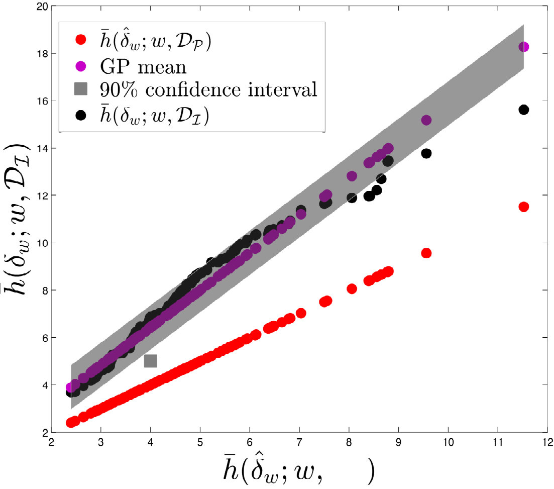 Figure 1
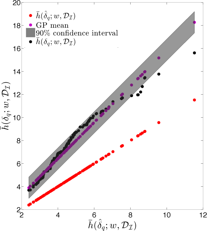 Figure 2
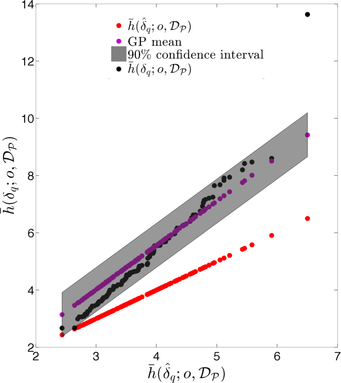 Figure 3
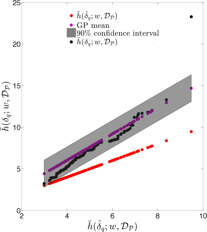 Figure 4
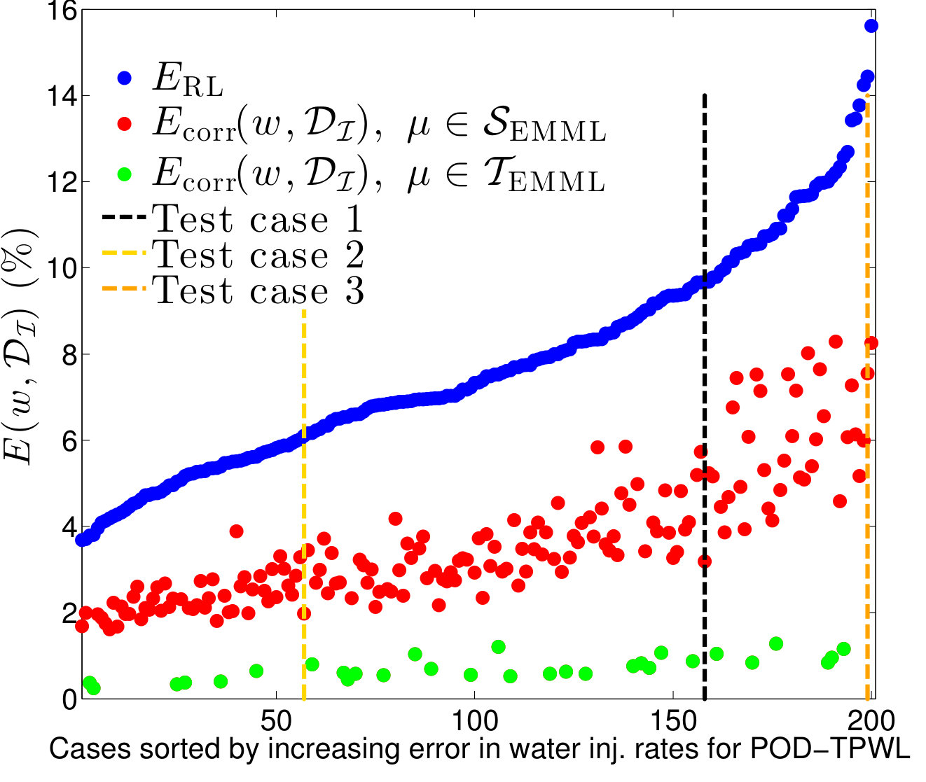 Figure 5
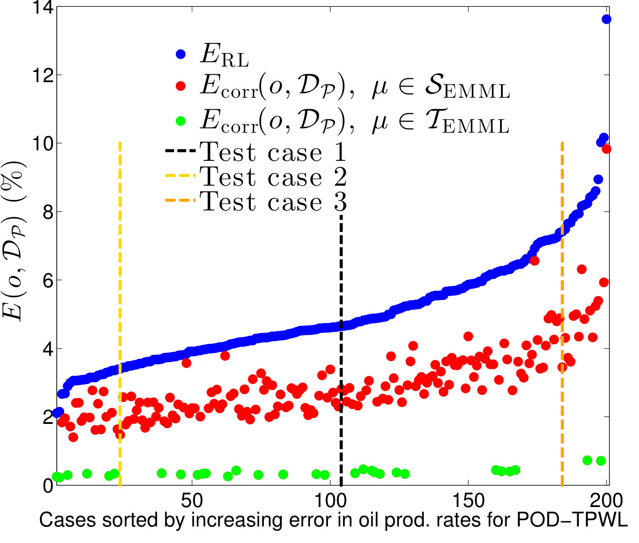 Figure 6
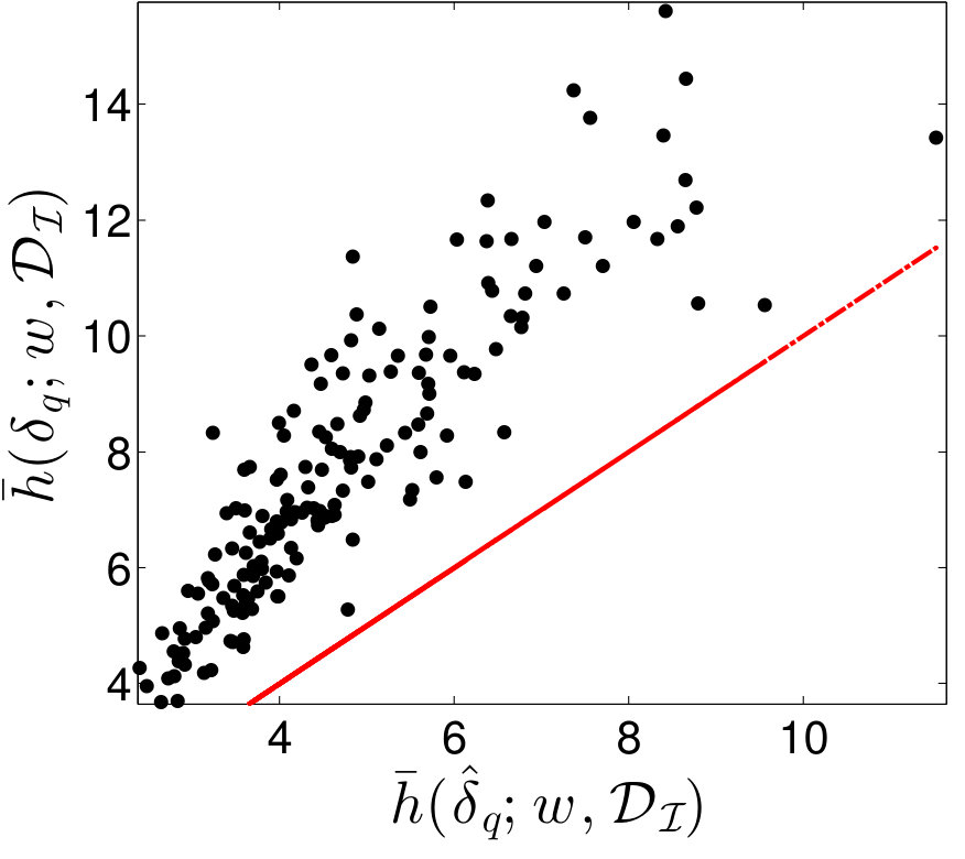 Figure 7
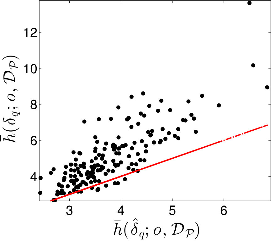 Figure 8
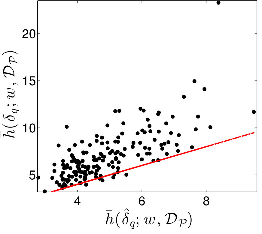 Figure 9
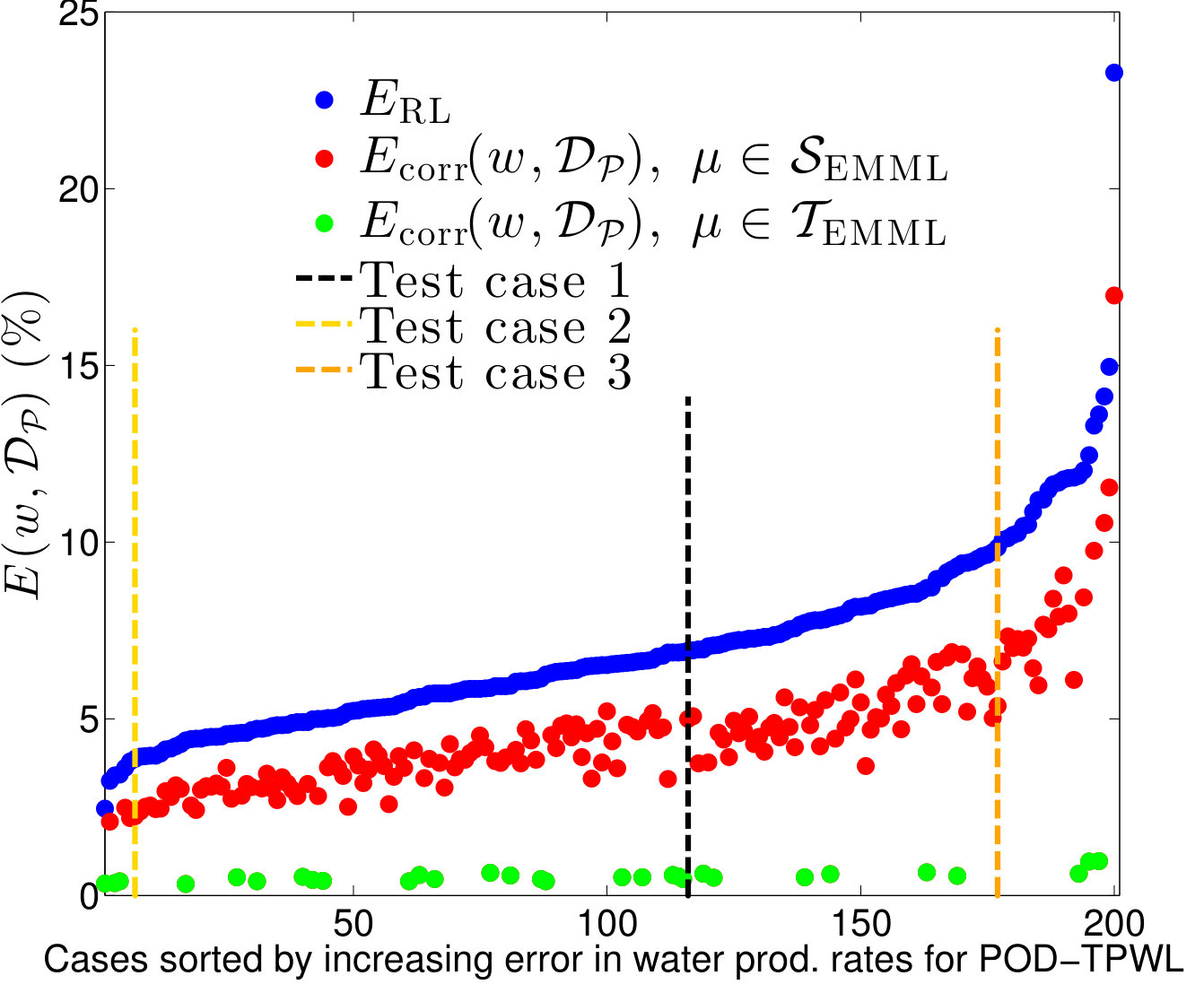 Figure 10
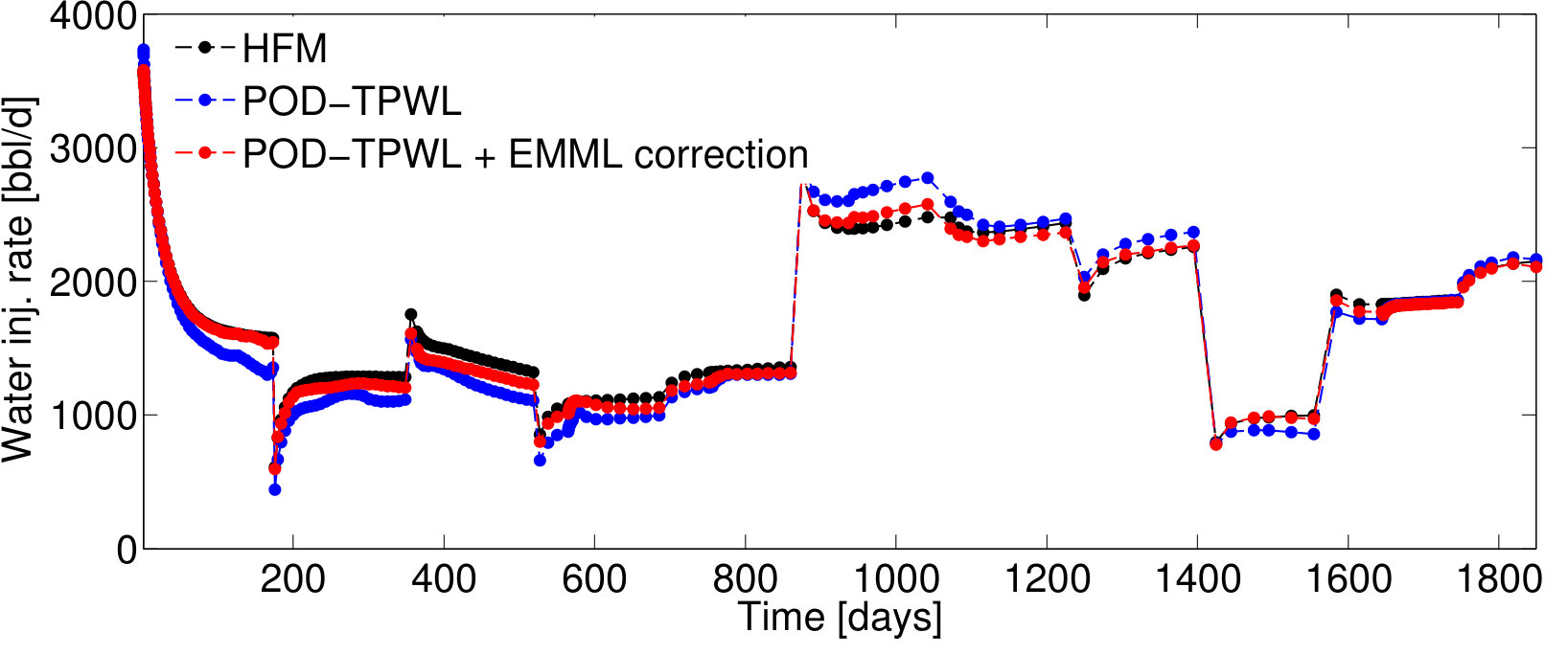 Figure 11
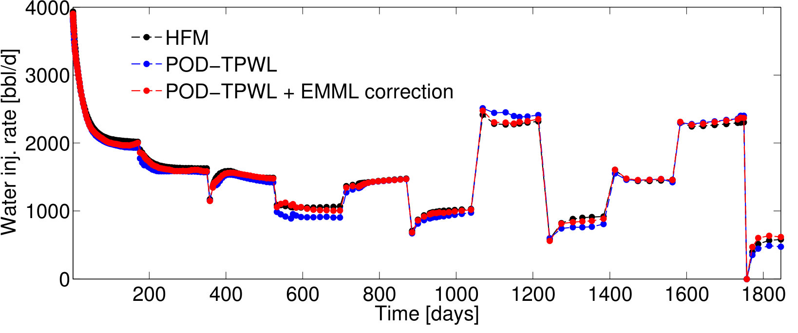 Figure 12
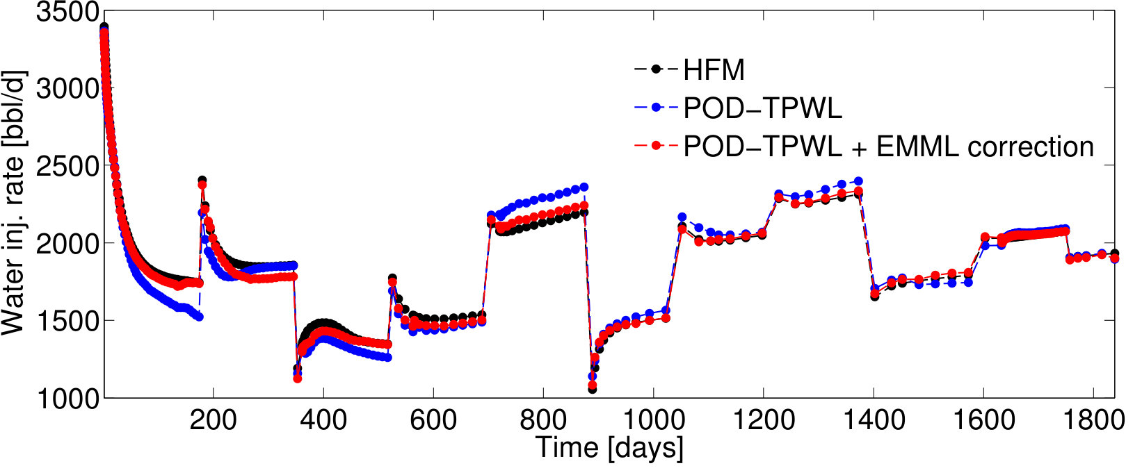 Figure 13
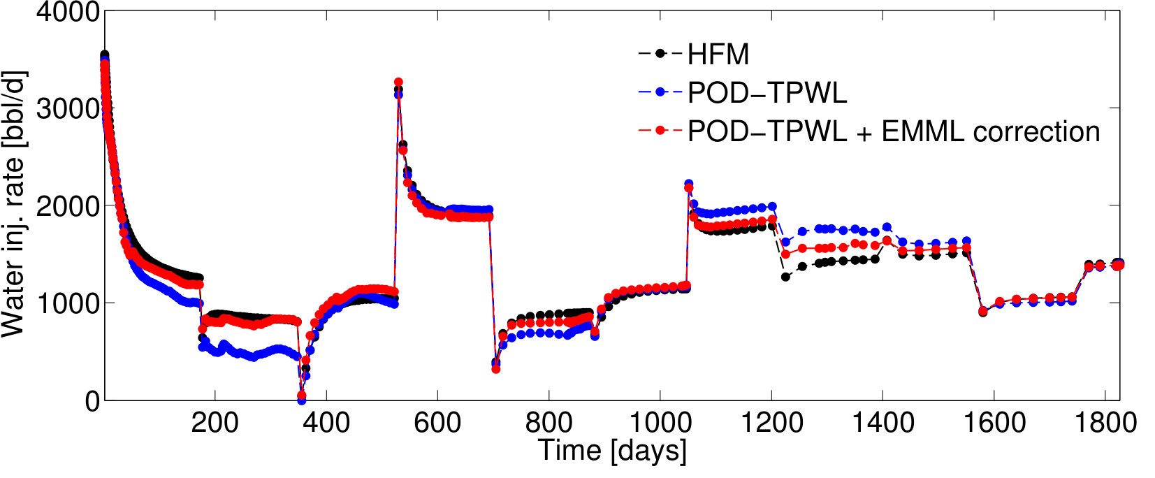 Figure 14
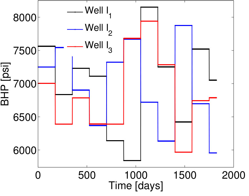 Figure 15
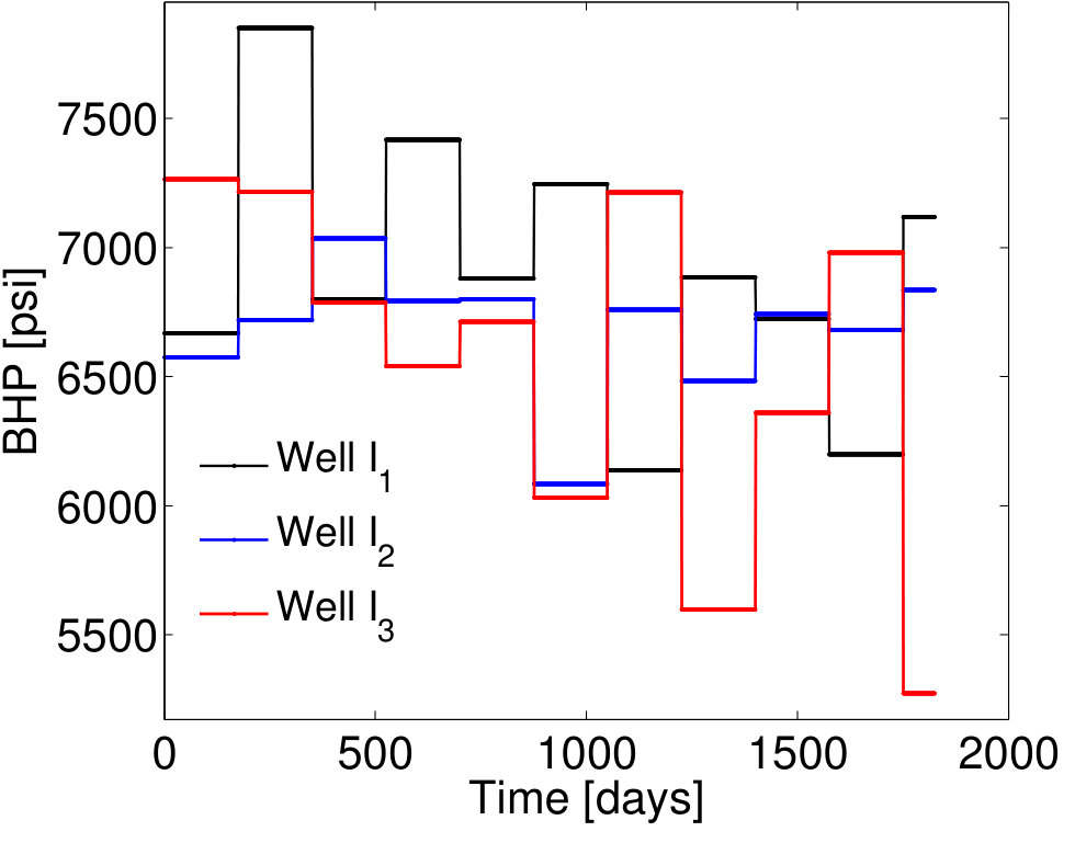 Figure 16
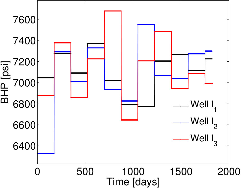 Figure 17
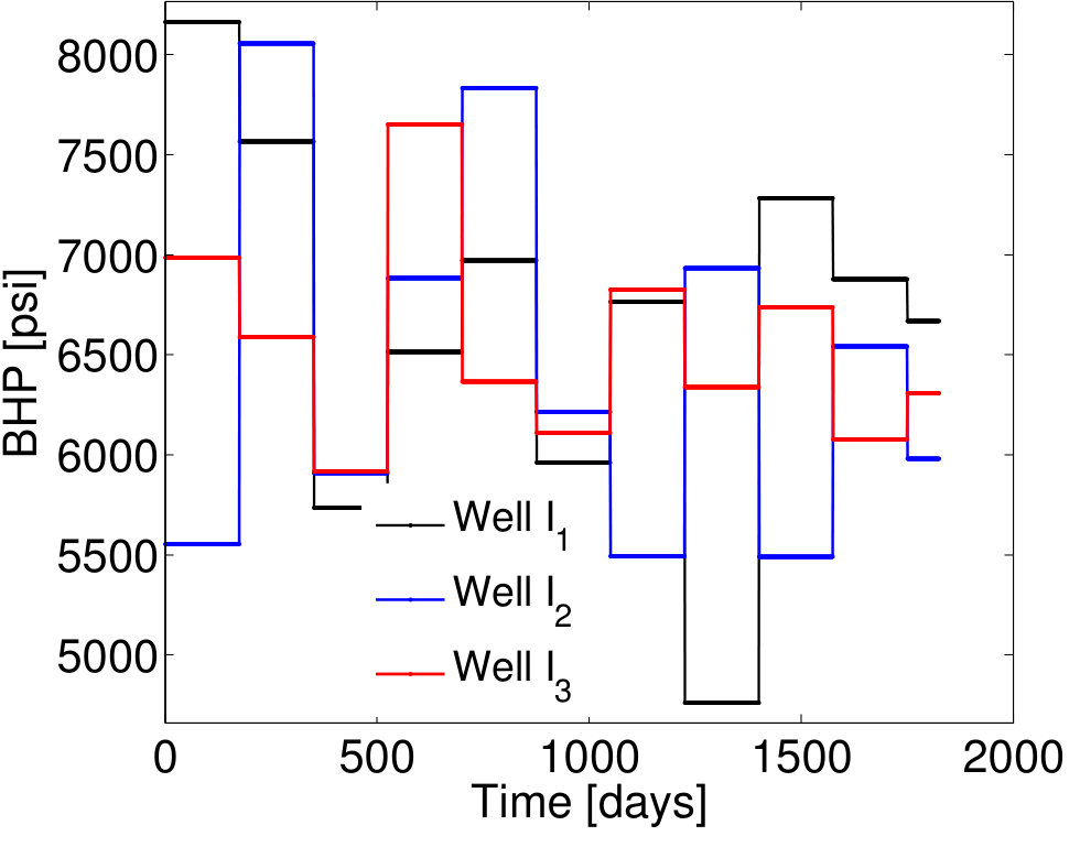 Figure 18
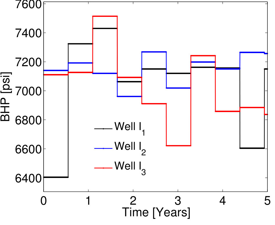 Figure 19
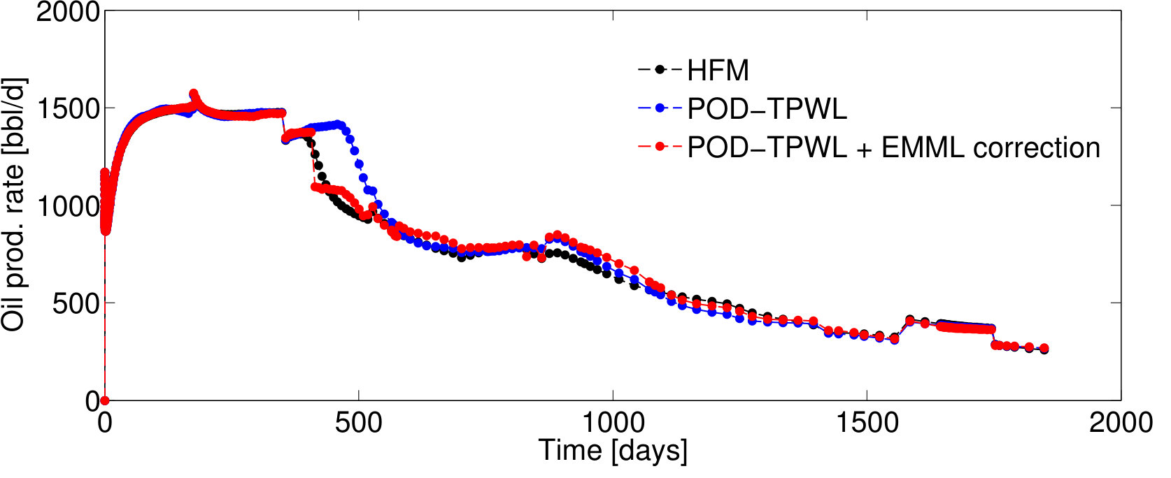 Figure 20
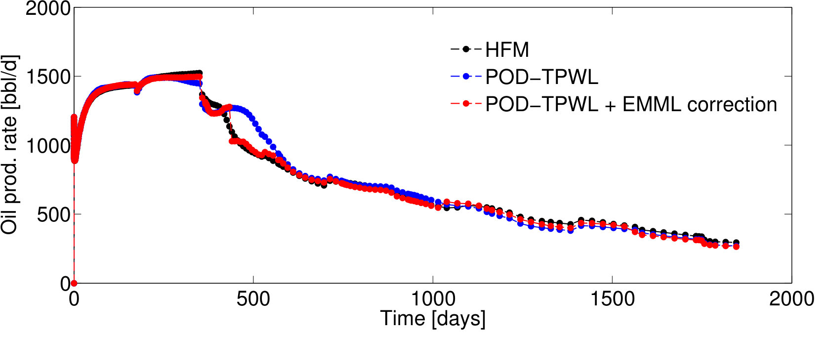 Figure 21
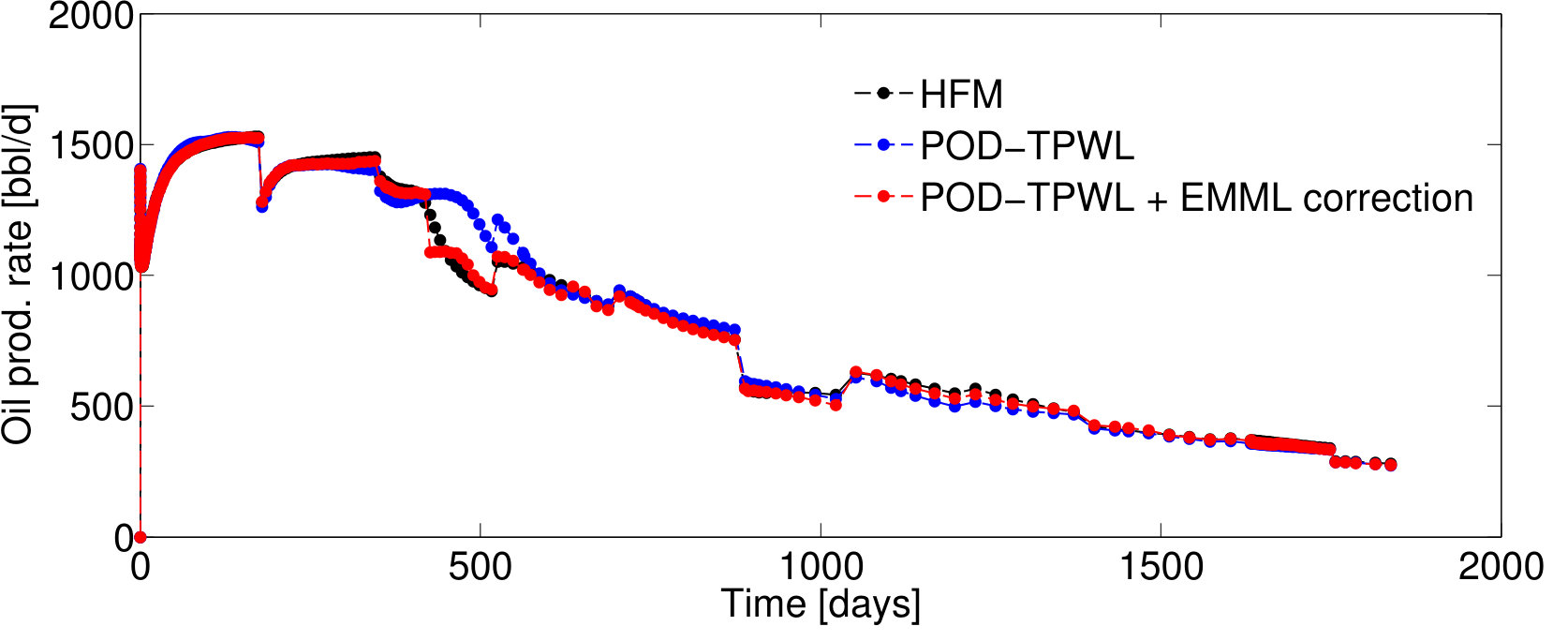 Figure 22
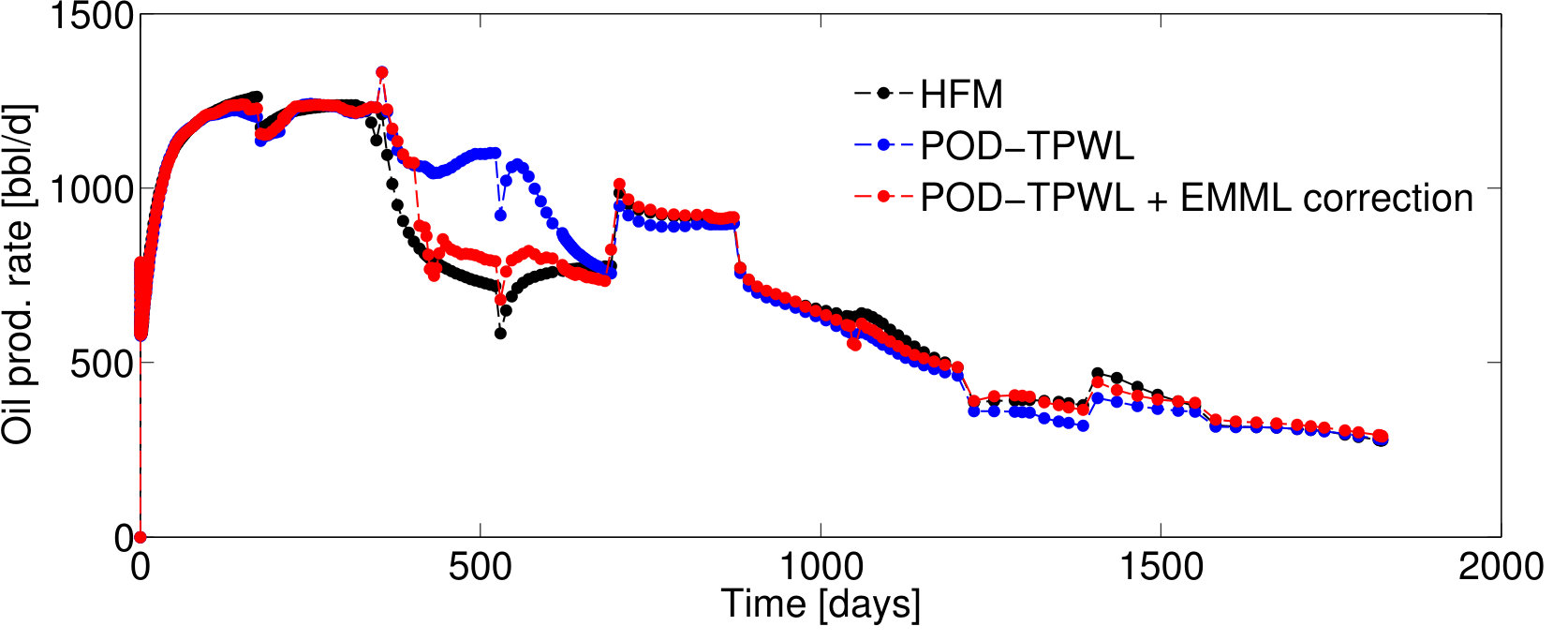 Figure 23
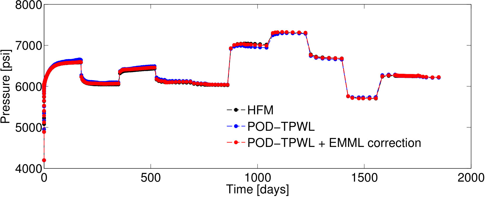 Figure 24
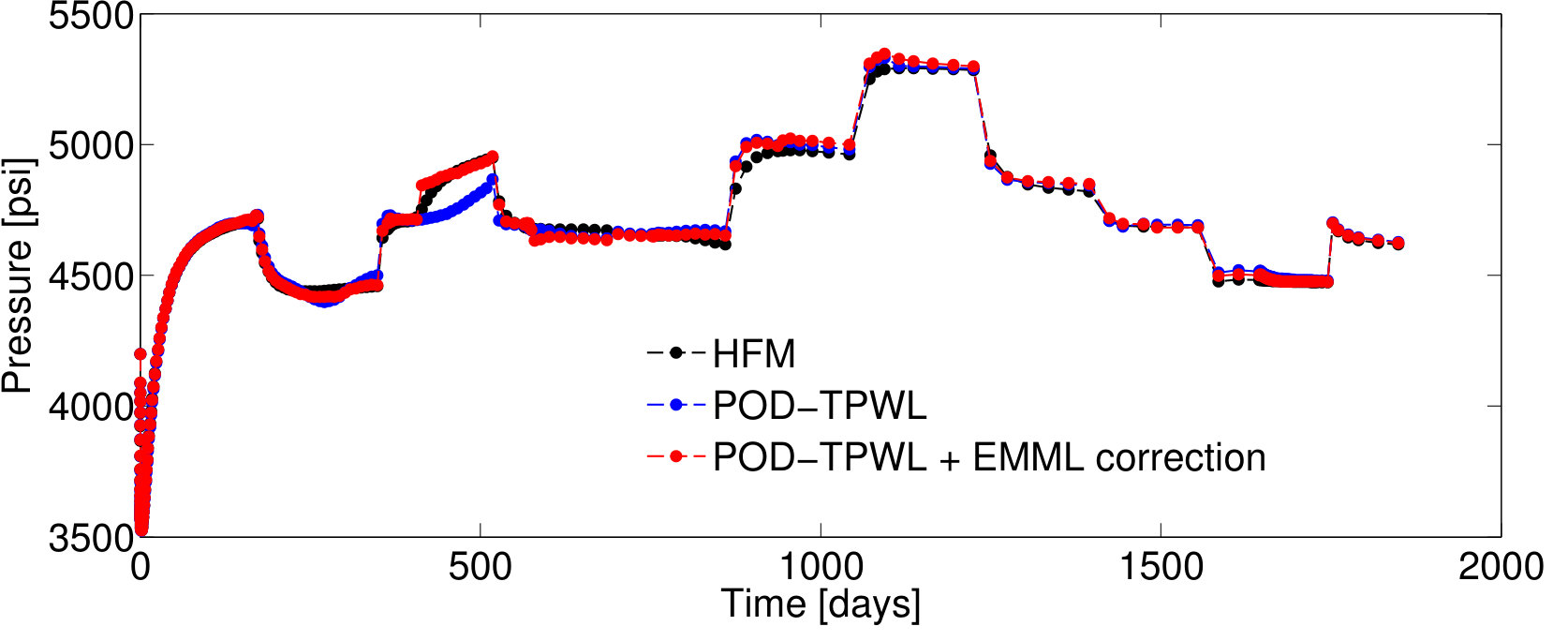 Figure 25
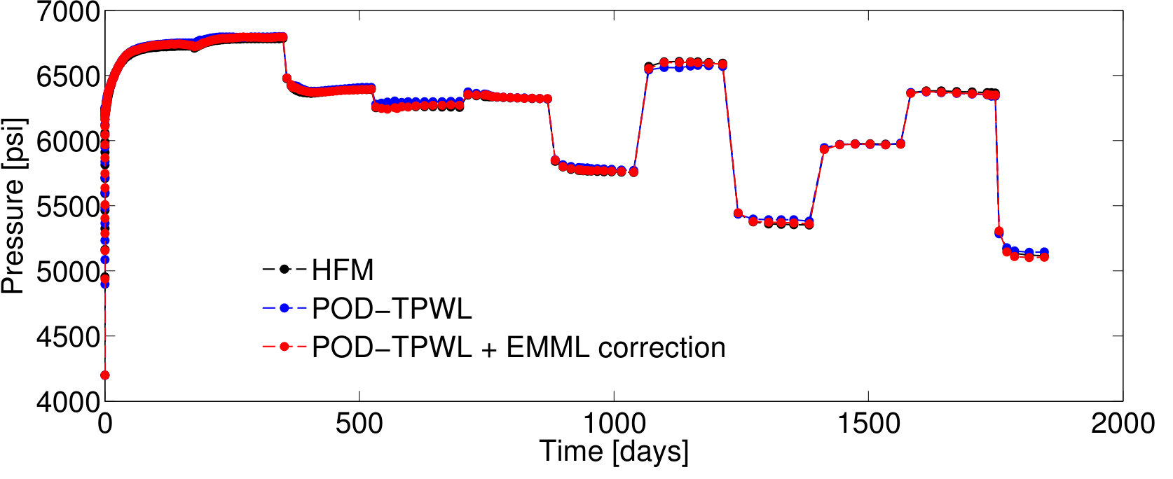 Figure 26
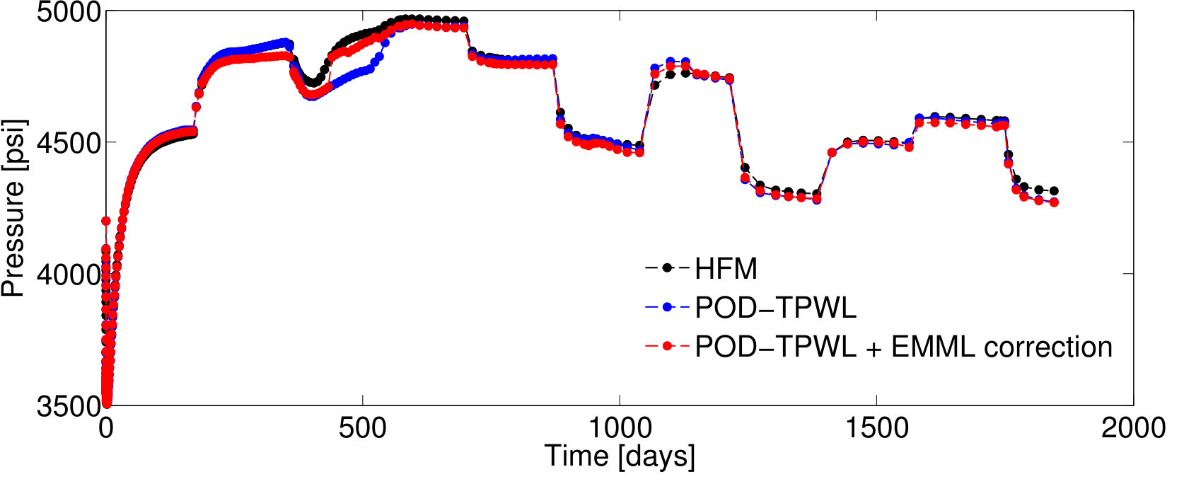 Figure 27
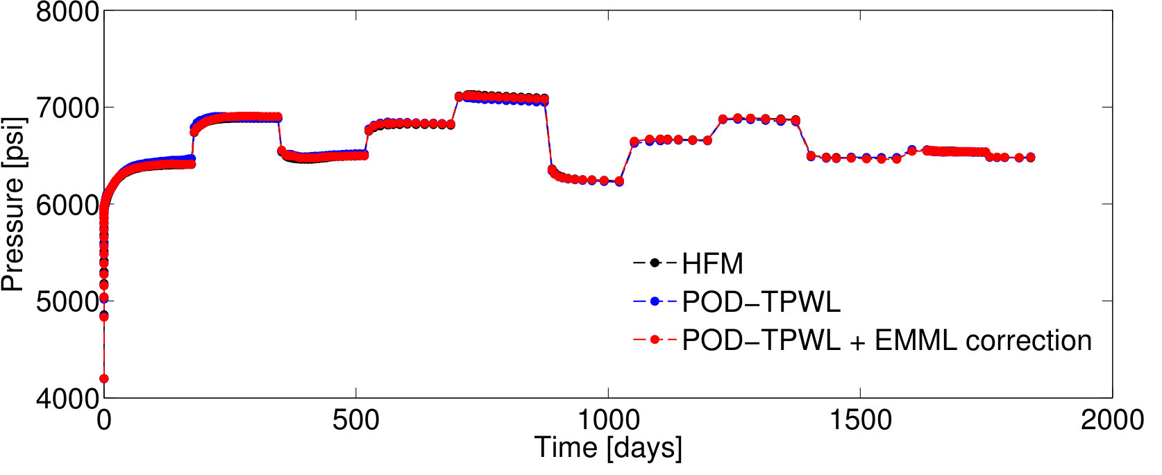 Figure 28
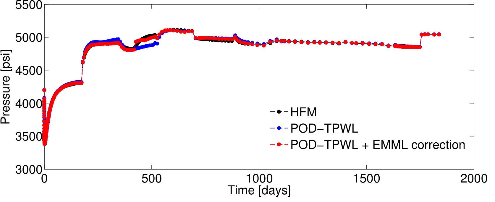 Figure 29
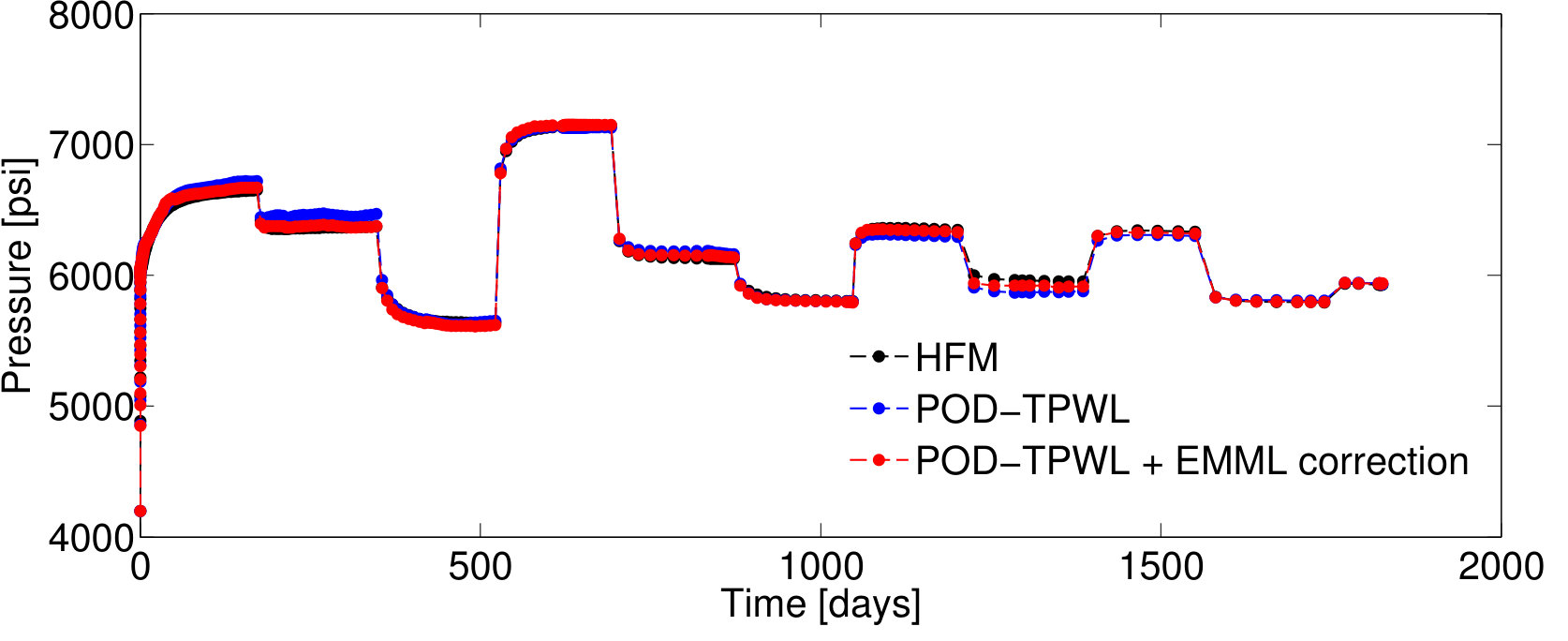 Figure 30
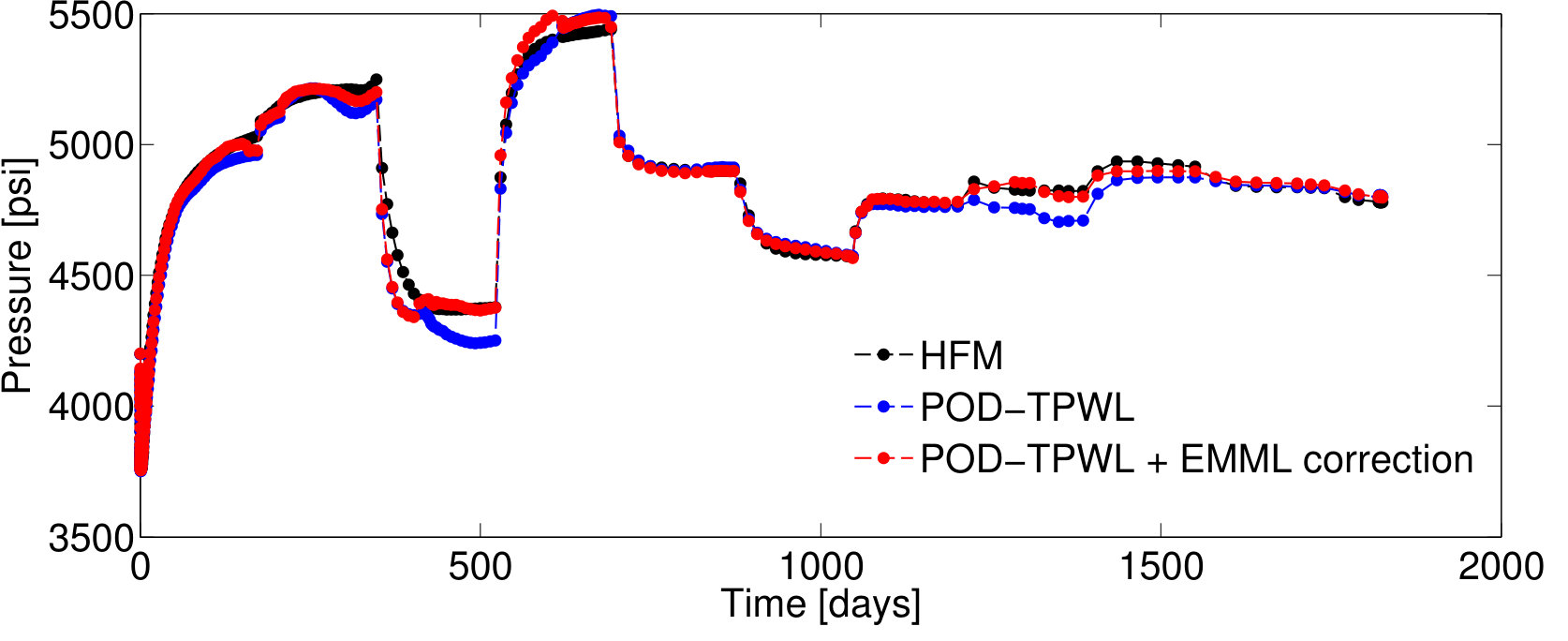 Figure 31
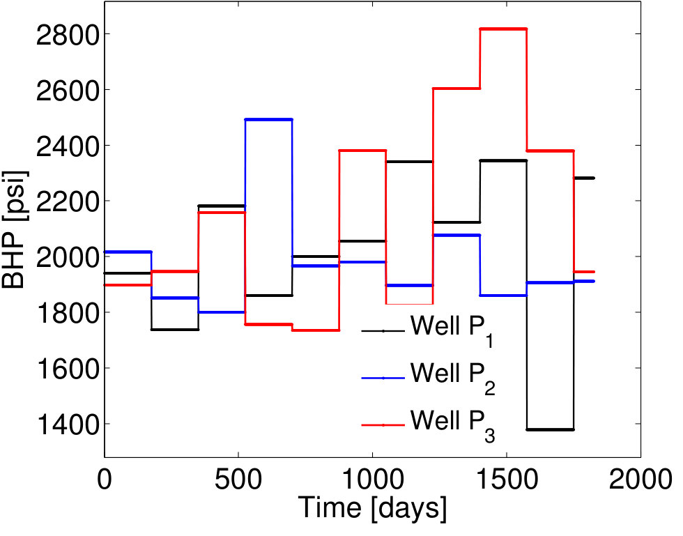 Figure 32
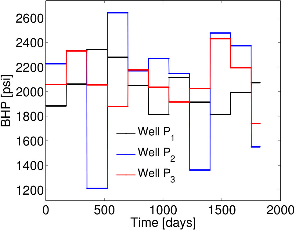 Figure 33
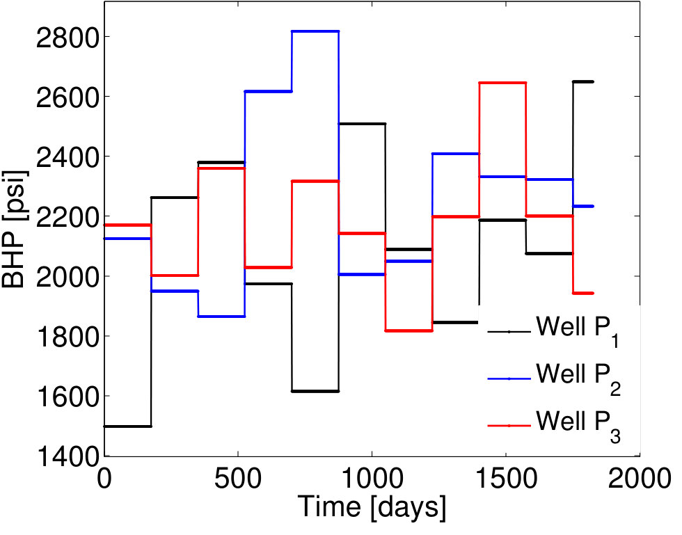 Figure 34
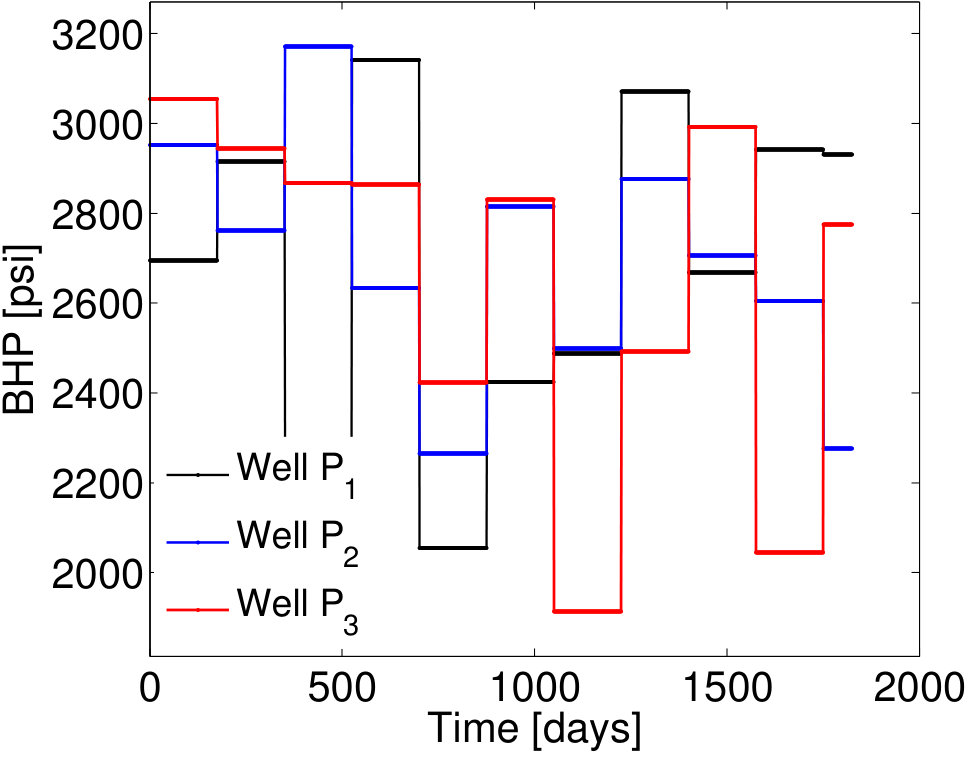 Figure 35
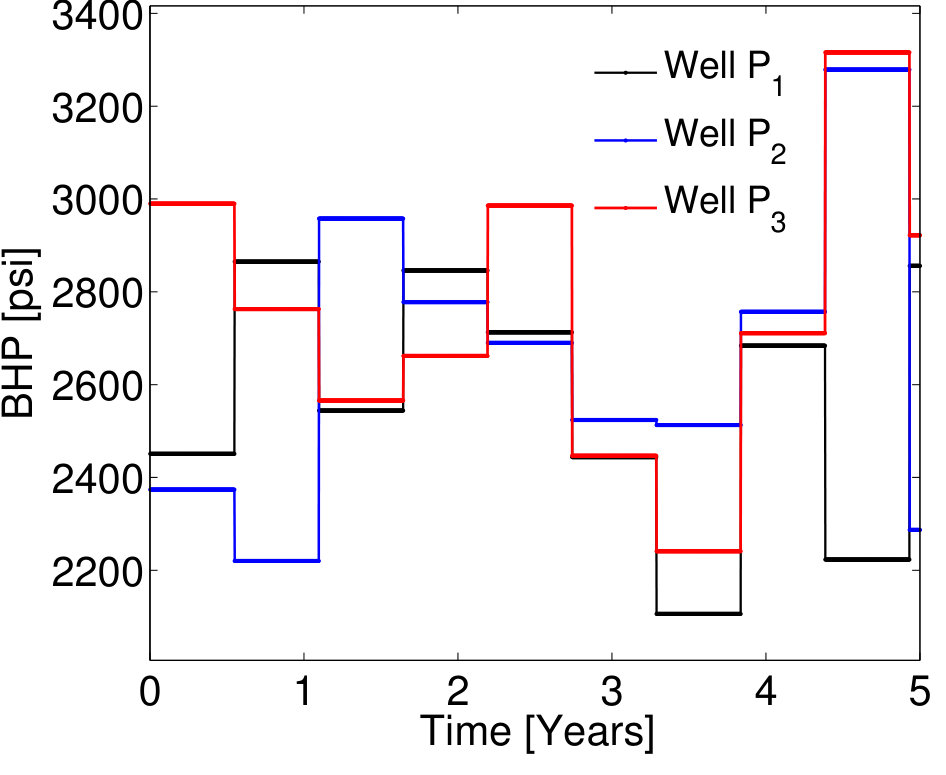 Figure 36
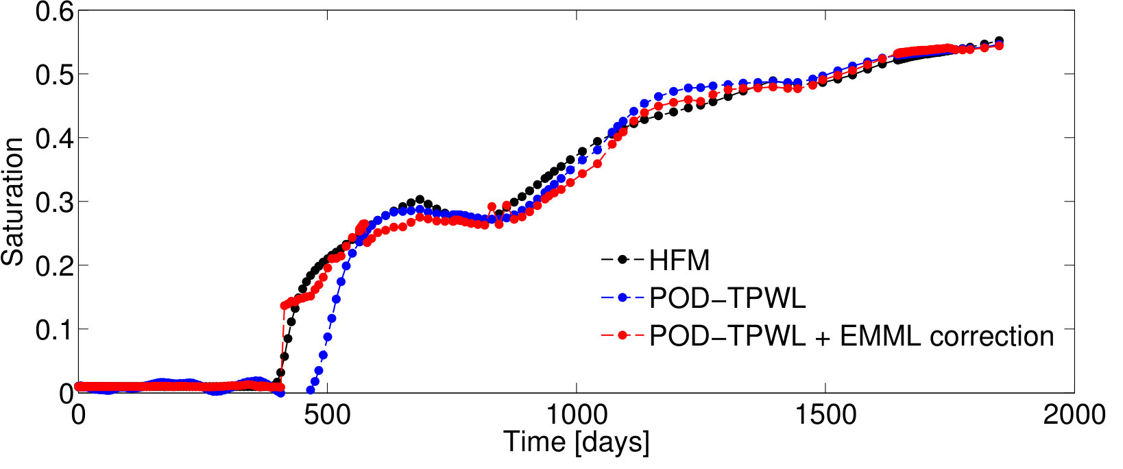 Figure 37
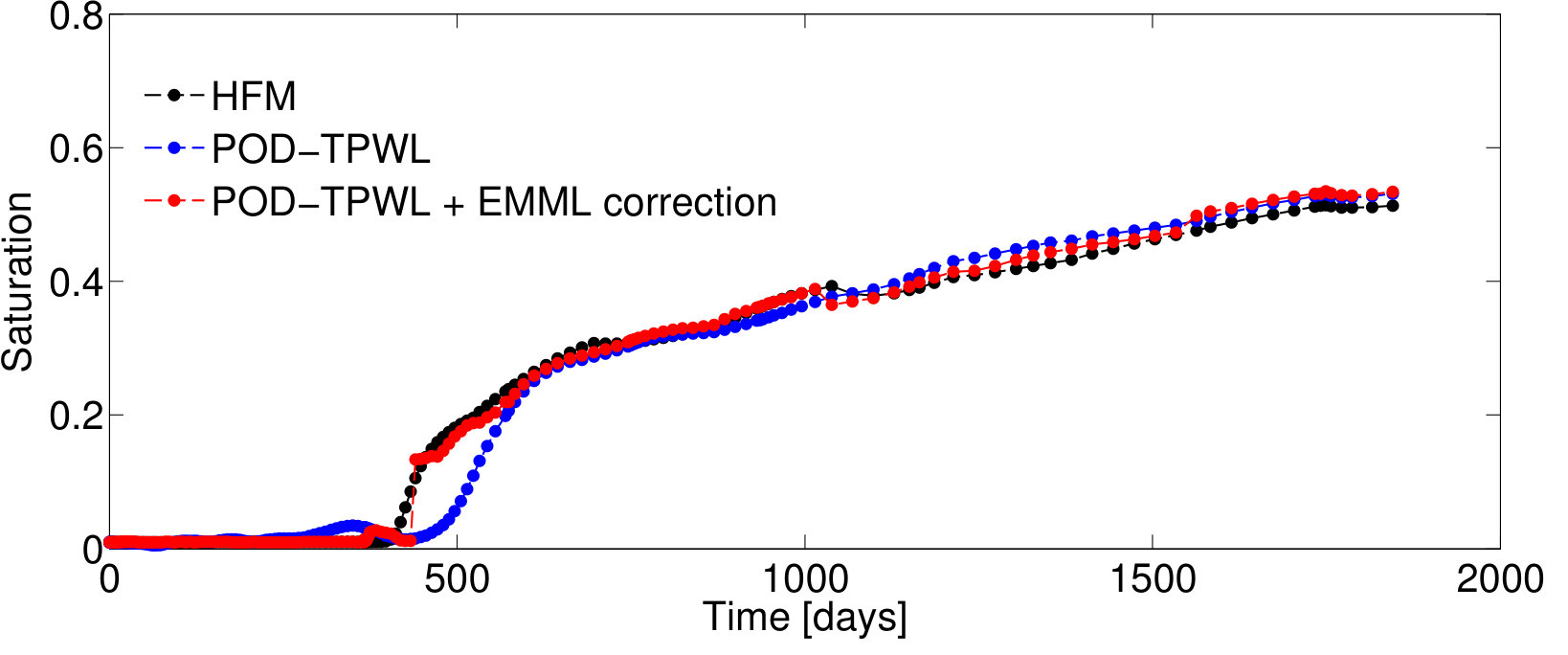 Figure 38
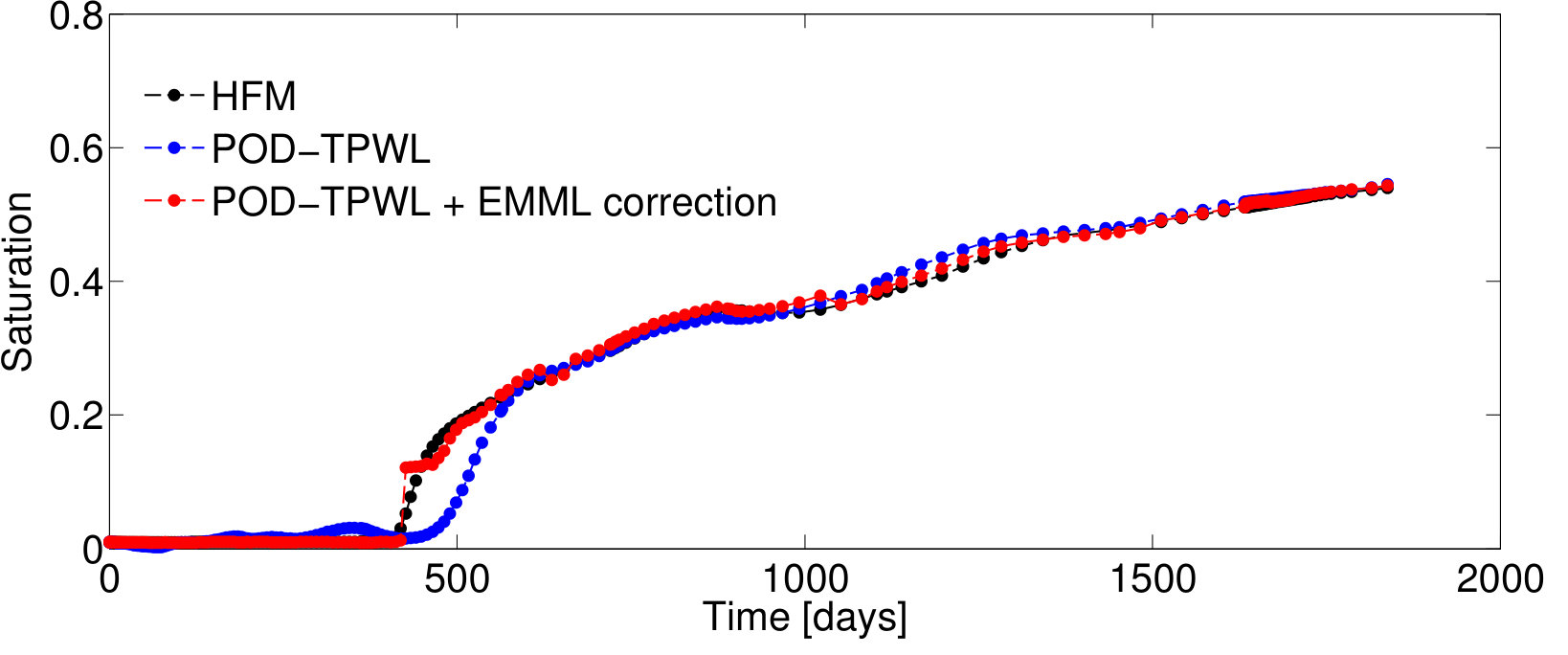 Figure 39
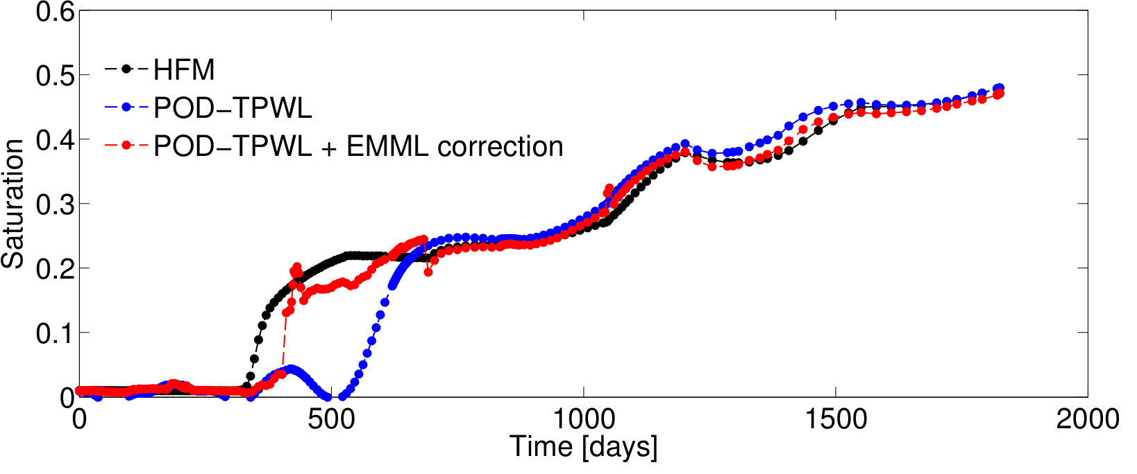 Figure 40
| No. | Feature | No. | Feature |
|---|---|---|---|
| 1. | 2. | ||
| 3. | 4. | ||
| 5. | 6. | ||
| 7. | 8. | ||
| 9. | 10. | ||
| 11. | 12. | ||
| 13. | 14. | ||
| 15. | 16. | ||
| 17. | 18. | ||
| 19. | 20. |
| No. | Feature | No. | Feature |
|---|---|---|---|
| 1. | 2. | ||
| 3. | , | 4. | |
| 5. | , | 6. |
| Method | |||
|---|---|---|---|
| POD–TPWL () | 4.5% | 6.3% | 6.6% |
| EMML correction (corr) | 2.8% | 4.4% | 3.7% |
| Method | |||||||
| (%) | (%) | (%) | |||||
| POD–TPWL () | 4.49 | 6.34 | 6.62 | ||||
| EMML correction (corr) | |||||||
| Approach | Locality | Regression | |||||
| 1 | 1 | 30 | classification | RF | 2.78 | 4.39 | 3.67 |
| 1 | 0 | 30 | classification | RF | 2.79 | 4.38 | 3.68 |
| 1 | 1 | 15 | classification | RF | 3.58 | 5.63 | 4.12 |
| 1 | 1 | 30 | classification | LS | 3.33 | 5.67 | 11.32 |
| 1 | 1 | 30 | clustering | RF | 3.23 | 5.22 | 3.68 |
| 1 | 1 | 30 | none | RF | 3.26 | 5.18 | 3.67 |
| 2 | 1 | 30 | classification | RF | 2.78 | 5.62 | 11.06 |
Peer Reviews
No public reviews on file for this paper yet. If you reviewed it on a platform where reviews are public (OpenReview, ICLR, NeurIPS, ICML), you can paste yours below so the community can read it here.
Videos
No videos yet. Explain this paper in a talk, walkthrough, or lecture? Add one.
Taxonomy
TopicsModel Reduction and Neural Networks · Probabilistic and Robust Engineering Design · Reservoir Engineering and Simulation Methods
\corraddr
Sumeet Trehan, Department of Energy Resources Engineering, Stanford University, 367 Panama Street, Stanford, CA 94035. Email: [email protected]
Error modeling for surrogates of dynamical systems using machine learning
Sumeet Trehan\corrauth
1
Kevin Carlberg and Louis J. Durlofsky
2
1
11affiliationmark: Department of Energy Resources Engineering, Stanford University, 367 Panama Street, Stanford, CA 9403522affiliationmark: Extreme-Scale Data Science and Analytics Department, Sandia National Laboratories, 7011 East Ave, MS 9159, Livermore, CA 94550
Abstract
A machine-learning-based framework for modeling the error introduced by surrogate models of parameterized dynamical systems is proposed. The framework entails the use of high-dimensional regression techniques (e.g., random forests, LASSO) to map a large set of inexpensively computed ‘error indicators’ (i.e., features) produced by the surrogate model at a given time instance to a prediction of the surrogate-model error in a quantity of interest (QoI). This eliminates the need for the user to hand-select a small number of informative features. The methodology requires a training set of parameter instances at which the time-dependent surrogate-model error is computed by simulating both the high-fidelity and surrogate models. Using these training data, the method first determines regression-model locality (via classification or clustering), and subsequently constructs a ‘local’ regression model to predict the time-instantaneous error within each identified region of feature space. We consider two uses for the resulting error model: (1) as a correction to the surrogate-model QoI prediction at each time instance, and (2) as a way to statistically model arbitrary functions of the time-dependent surrogate-model error (e.g., time-integrated errors). We apply the proposed framework to model errors in reduced-order models of nonlinear oil–water subsurface flow simulations, with time-varying well-control (bottom-hole pressure) parameters. The reduced-order models used in this work entail application of trajectory piecewise linearization in conjunction with proper orthogonal decomposition. When the first use of the method is considered, numerical experiments demonstrate consistent improvement in accuracy in the time-instantaneous QoI prediction relative to the original surrogate model, across a large number of test cases. When the second use is considered, results show that the proposed method provides accurate statistical predictions of the time- and well-averaged errors.
keywords:
surrogate model, error modeling, machine learning, nonlinear dynamical system, POD–TPWL
1 Introduction
Computational simulation is being increasingly employed for real-time and many-query problems such as design, optimal control, uncertainty quantification, and inverse modeling. However, these applications require the rapid and repeated simulation of a (parameterized) computational model, which often corresponds to a discretization of partial differential equations (PDEs) that can be nonlinear, time dependent, and multiscale in nature. Accurate predictive models can therefore incur substantial computational costs. While recent advances in parallel computing have reduced simulation times for high-fidelity models, the rapid, repeated simulation of such models remains a bottleneck in many applications.
This computational challenge has motivated the development of a wide range of surrogate-modeling methods. Surrogate models—which can be categorized as data fits, lower-fidelity models, or reduced-order models (ROMs)—are approximations of high-fidelity models (HFMs) that aim to provide large computational savings while preserving accuracy. Unfortunately, these models often introduce non-negligible errors due to the assumptions and approximations employed in their construction, and these errors can have deleterious effects on the resulting analysis. Thus, to more rigorously employ surrogate models, it is critical to quantify the errors they introduce. Without reliable error quantification —which can be accomplished via statistical approaches, rigorous error bounds, error indicators, or error models—the accuracy of surrogate-model predictions is unknown, and the trustworthiness of the resulting analysis may be questionable.
For this reason, researchers have developed a variety of methods for quantifying surrogate-model errors. Data-fit surrogate models construct a deterministic function (e.g., polynomial fit [1], artificial neural network [2]), or stochastic process (e.g., Gaussian process/kriging [3, 4]) that explicitly approximates the mapping from the model input parameters to the model output quantity/quantities of interest (QoI). For this class of surrogate model, statistical approaches such as the value [5], cross validation [5, 6], confidence intervals, and prediction intervals [5, 6] can be applied to quantify surrogate error. When the data fit corresponds to a stochastic-process model, the prediction variance can be applied to quantify the uncertainty in the prediction directly [7, 8]. Although data-fit surrogates are nonintrusive to implement (they require only ‘black-box’ queries of the HFM), their predictions are not physics based, which can lead to inaccurate predictions, especially for high-dimensional input-parameter spaces. For this reason, many applications demand more sophisticated physics-based surrogates such as lower-fidelity or reduced-order models.
Lower-fidelity models are physics-based surrogates that apply simplifications to the original HFM, such as coarser discretizations, lower-order approximations or linearization, or they neglect some physics. In this case, one approach for quantifying the error would be to explicitly model the error via a ‘data-fit’ mapping between input parameters and lower-fidelity-model error. These approaches—which have been pioneered in the field of multifidelity design optimization—typically enforce ‘global’ zeroth-order consistency between the corrected low-fidelity-model QoI and the HFM QoI at training points [9, 10, 11, 12, 13, 14, 15], or ‘local’ first- or second-order consistency at trust-region centers [16, 17]. Unfortunately, in the context of dynamical systems (which we consider in this work), such corrections are only applicable to scalar-valued QoI (e.g., time-averaged quantities). Quantifying the error in time-dependent quantities has been largely ignored, with the exception of recent work that interpolates time-dependent error models in the input-parameter space [18]. In addition, the error may exhibit a complex or oscillatory dependence on the input parameters, which adds further challenges in high-dimensional input-parameter spaces and can cause the approach to fail [13, 19]. Alternatively, adjoint-based error estimation (i.e., dual-weighted-residual error indicators) can also be applied to approximate QoI errors in the context of coarse finite-element [20, 21, 22, 23], finite-volume [24, 25, 26], and discontinuous Galerkin [27, 28] discretizations. Unfortunately, for dynamical systems, dual-weighted residuals require an additional (time-local or time-global) dual solve, which can incur a non-negligible additional cost.
Projection-based ROMs apply projection to reduce the dimensionality of the equations governing the HFM. Typically, the low-dimensional bases are derived empirically by evaluating the HFM at training points or by performing other analyses, e.g., solving Lyapunov equations or computing a Krylov subspace. ROM error is typically estimated by deriving rigorous a priori and a posteriori error bounds for the state, QoI, or transfer function; such bounds have been derived for the reduced-basis method [29, 30, 31], system-theoretic approaches (e.g., balanced truncation, rational interpolation) [32], and proper-orthogonal-decomposition (POD) Galerkin [33, 34] and least-squares Petrov–Galerkin (LSPG) [35] methods; see, e.g., [36] for a review. However—for dynamical systems—such error bounds typically grow exponentially in time, causing the bound to significantly overpredict the error [37], which can limit the practical utility of these bounds. Note that the approaches developed for quantifying the low-fidelity-model error could also be adopted to quantify ROM errors [13, 38], as ROMs can be interpreted as lower-dimensional models with empirically derived basis functions.
To address the above issues in the context of quantifying ROM errors, Drohmann and Carlberg [19] devised the reduced-order-model error surrogates (ROMES) approach , which can be considered an error-modeling approach, as it constructs a Gaussian process that maps error indicators (e.g., error bounds, residual norms, dual-weighted residuals) produced inexpensively by the ROM to a distribution over the ROM QoI error. This study demonstrated that—even in the presence of high-dimensional input-parameter spaces—the ROM produces a small number of inexpensively computable error indicators that can be employed to derive accurate, low-variance predictions of the ROM error. Follow-on work also investigated the use of statistical modeling and regression methods to model ROM errors from indicators [39]. While promising, the ROMES approach requires the user to hand-select the error indicators that are most strongly correlated with the ROM error; i.e., feature selection is left to the user. This task can be challenging in general applications, as the user may not have strong a priori knowledge of which (small number of) features inform the error. Further, the ROMES method was demonstrated only on a stationary (i.e., steady-state) problem, and its extension to dynamical systems is nontrivial. Finally, application of the ROMES method to other physics-based surrogates (e.g., coarsened or upscaled models) is not obvious, as different error indicators will likely be required for such surrogates.
In this paper, we propose a machine-learning-based framework for modeling the error introduced by physics-based surrogate models of dynamical systems. The approach applies statistical techniques for high-dimensional regression (e.g., random forests) to map a large set of inexpensively computed quantities or features generated by the surrogate model to a prediction of the time-instantaneous surrogate-model QoI error. This method is referred to as error modeling via machine learning (EMML). In contrast to the ROMES method, the proposed EMML approach enables a large number of potential error indicators to be included in the candidate feature set and thus does not require the user to manually select a small number of features that inform the error, which can be challenging as mentioned above. Thus, feature selection is included in the process of constructing the error model, and extension to multiple types of physics-based surrogates is straightforward—we assume only that the surrogate produces a large set of features that can be mined for potential error indicators.
While the proposed framework can be applied to any surrogate model in principle, in this study we apply the method to model errors introduced by a TPWL ROM [40, 41, 42, 43] applied with a proper orthogonal decomposition (POD) basis and LSPG projection [44, 35], which we refer to hereon as POD–TPWL. We employ this ROM rather than other approaches (e.g., (D)EIM with POD–Galerkin, GNAT) because TPWL is less intrusive: it simply requires extracting linear operators (i.e., Jacobians of the residual with respect to the current state, previous state, and controls) from the HFM simulation code during the offline training stage, and it is entirely independent of the HFM simulation code during the online stage. This particular ROM was also employed in previous subsurface-flow studies involving oil–water and oil–gas compositional problems [45, 46, 47]. At each time step during test simulations, POD–TPWL performs linearization around the nearest training solution; LSPG projection is then applied—with a low-dimensional POD basis—to reduce the dimensionality of the linearized system. While the approach has been shown to yield speedups [42, 43, 45], POD–TPWL incurs non-negligible errors due to the approximations it introduces, namely (1) linearization error, and (2) ‘out-of-plane error’ [34] arising from employing a low-dimensional POD trial subspace, (3) ‘in-plane error’ arising from projection, and (4) error propagated from the previous time step. See [46] for further discussion of POD–TPWL error. We aim to apply the proposed EMML framework to model the QoI error resulting from these approximations.
Finally, we note that while machine learning and its application across various disciplines have been extensively studied, the use of machine learning within the domain of physics-based modeling and simulation is relatively new, although it is quite promising [48, 49]. In the context of improving surrogate-model predictions, researchers have recently investigated the use of machine learning techniques to identify (via classification) the spatial locations for high low-fidelity-model error [50]. Machine learning has also been used to quantify the inherent error with kriging data-fit surrogates [51] and to derive improved closure models in the context of computational fluid mechanics [52, 53, 54, 55, 56]. Machine learning was also applied to derive the source term for the transport of an intermittency variable while transitioning from laminar to turbulent flow [57]. Similarly, regression techniques (e.g., LASSO [58]) have been used to calibrate and infer uncertainties in viscosity-model coefficients for transonic flow applications [59]. We note that although machine learning has been used in a post-processing step to identify the physical regions of high surrogate-model error [50], to our knowledge, the direct approximation of error through construction of a regression model has not been pursued.
The paper proceeds as follows. In Section 2 we describe the general EMML framework. Following the definition of the error in the QoI, we introduce four methods to map this error to a set of inexpensively computed features using high-dimensional regression techniques. The particular HFM (subsurface flow) and surrogate model (POD–TPWL) considered as an application are discussed in Section 3. In Section 4, we present numerical results for modeling the POD–TPWL error in flow quantities driven by time-varying control variables over a large number of test cases. Different algorithmic treatments are also considered. A summary and suggestions for future work are provided in Section 5. Appendices A and B present descriptions of random-forest and LASSO regression.
2 General Problem Statement
In this section, we describe the overall EMML framework for error modeling. We begin by introducing both the high-fidelity model (HFM) and the surrogate model in a general setting.
2.1 Dynamical-system high-fidelity model
Given input parameters , we assume that the HFM generates a time history of states , , and a scalar-valued output QoI that depends on the state, i.e.,
[TABLE]
Here, with is a sampling matrix comprising selected rows of the identity matrix. This operator extracts the elements of the state vector required to compute the QoI .
2.2 Dynamical-system surrogate model
We assume that the inexpensive surrogate model generates a time history of surrogate-model states , (ideally with ), given the input parameters . The QoI can be computed from the surrogate model states z using the function . Our critical assumption is that the surrogate model also produces auxillary data in the form of a time history of ‘features’ , , given these parameters . The surrogate model is described as follows:
[TABLE]
Here, denotes a prolongation operator that transforms the surrogate model state into the elements of the high-fidelity state required to compute the QoI. The decision of what to include in the set of features is motivated by the underlying form of , as discussed in Section 3.3. For notational simplicity, from hereon we use in place of .
2.3 Error modeling
Our objective is to predict the error in the QoI at each time step , which we define as
[TABLE]
where , , denotes the QoI computed using the HFM at time instance , and denotes the QoI computed using the surrogate model at time instance . We propose to approximate this QoI error as , by constructing error surrogates using high-dimensional regression methods developed in the context of machine learning.
In particular, we propose four regression-based approaches that construct a mapping from the surrogate-model features to a QoI-error prediction . While it is possible to construct an error prediction as a function of only the input parameters , this approach can fail due to the oscillatory behavior of certain surrogate-model errors in the input space [13, 19], as discussed in the Introduction. For notational simplicity, hereon .
2.3.1 Method 1: QoI error.
The first method models the nondeterministic mapping as a sum of a deterministic function , and nondeterministic noise as follows:
[TABLE]
Here, is a zero-mean random variable that accounts for potentially unknown features, deficiencies in the model form of , and the error introduced due to sampling variability. Thus, denotes irreducible error induced by the error model Equation (7), and it may in principle depend on the features (i.e., ); this heteroscedasticity can occur, for example, when the mean and variance of the predicted error are larger for larger-magnitude features. For simplicity, we neglect this dependence in the current study.
We note that employing the error model in Equation (7) allows us to (1) approximate the form of using data, which in turn enables us to express the error in the QoI as a function of the features only, and (2) account for the possibility that the same feature vector may yield different values of the QoI error, i.e., with but .
Next, we construct a model of the function , such that , . This model allows the error to be approximated as a function of the features as
[TABLE]
Note that we consider modeling as a prediction problem rather than as a time-series-analysis problem. This is because, in the problem under consideration, we perform numerical experiments for different input-parameter instances over the same time interval. Thus, we include time in the feature set, as described in Section 3.3. Implicitly, we assume that samples are independent and identically distributed (i.i.d.), with each sample corresponding to the quantity at a given time step.
2.3.2 Method 2: relative QoI error.
In many cases, the QoI errors can exhibit a wide range of observed values. This can make the machine-learning task more challenging, as the associated regression model must be predictive across this entire range of values. To address this, we can instead apply regression to the relative QoI errors—which typically exhibit a narrower range of values—and subsequently approximate the QoI errors in a postprocessing step.
We define the relative QoI error at time step by
[TABLE]
and—following Method 1—express the mapping as
[TABLE]
where is an unknown deterministic function. We model by constructing an approximation such that , , . This allows the approximated relative error to be expressed as
[TABLE]
From Equation (6), it follows that
[TABLE]
which allows the QoI error to be related to the relative QoI error by
[TABLE]
Therefore, we can model the QoI error as from the relative QoI regression model in a postprocessing step as
[TABLE]
2.3.3 Method 3: state error.
As an alternative to modeling the QoI error, we can model the error in the relevant state(s), and then use this quantity to approximate the QoI error. This method is advantageous when the QoI error exhibits a more complex behavior than the state error, as may be the case for highly nonlinear QoI. We denote the error in the sampled state at time step by
[TABLE]
where and denotes the th element of the vector-valued argument.
The next steps follow closely the derivation of Method 1. As before, we model the mappings as
[TABLE]
where , , denote unknown deterministic functions that allow the state-variable errors to be computed as a function of the features. Analogous to Equation (7), we construct regression models , such that , , , . This model allows the approximated state error to be expressed as
[TABLE]
Note that instead of pursuing multi-response multivariate regression, we execute independent multivariate regressions, i.e., we construct a unique and independent mapping for each of the sampled states. Because the QoI error can be expressed as
[TABLE]
we can model the QoI error from the modeled state error in a postprocessing step as
[TABLE]
2.3.4 Method 4: relative state error.
Finally, if the errors in a particular sampled state exhibit a wide range of observed values, we can construct a regression model for the relative state error, which we define as
[TABLE]
with , and subsequently use this model to predict the QoI error. Analogous to Methods 1–3, we construct a regression model, which maps the features to the relative error in the sampled state , thus enabling the computation of the approximated relative error . Analogous to Method 2, we relate the relative error in the sampled state to the actual error. After using Method 3 or Method 4 or some combination thereof to compute the value of , we apply Equation (19) to determine the QoI error model .
2.4 Training data
Each of the four methods described above entails the use of a regression model to predict the output (response)—which corresponds to the actual or relative error in the QoI or in the sampled state—given the inputs (features). Constructing any such regression model relies on training data. We denote points in the input-parameter space used to collect these data as
[TABLE]
where , denotes the th EMML training instance of the input parameters, and denotes the number of training points.
Next, we simulate both the HFM and the surrogate model for input-parameter instances in the training set . This produces the EMML training data, which comprise errors , and features over all time steps and training simulations, i.e.,
[TABLE]
As mentioned previously, we assume that the associated samples are i.i.d. In the following, we denote a general training error by , .
2.5 Regression-model locality
As an alternative to constructing a single global regression function, , or , that is valid over the entire feature space, we can instead construct multiple ‘local’ regression models that are tailored to particular physical regimes or feature-space regions with the intent of improving prediction accuracy. To realize this, we partition the training data into subsets corresponding to different feature-space regions and construct separate regression functions for each subset. We consider two methods for determining regression-model locality: classification and clustering.
Classification is a supervised machine learning technique [6] that predicts the label (or category) to which an observation belongs. In this work it entails constructing a statistical model from EMML training data containing samples whose category membership is known, along with categorization criteria for those samples. In the current context, we propose applying classification using ‘classification features’ that may in general be different from the EMML features . We employ these features to identify the subsets of the EMML training data associated with different physical regimes of the problem, for which different regression models are appropriate. Then, given a new observation for which we require error prediction, we first identify its category using the classification model, and subsequently apply the associated local regression model for error prediction.
Clustering is an unsupervised machine learning method [6] that can be applied to partition the training data according to the (e.g., Euclidean) distance in feature space between the training samples. We propose partitioning feature space (or a lower-dimensional space embedded in feature space computed, e.g., via principal component analysis) according to the Voronoi diagram produced by the cluster means. In this work, we employ -means clustering where the number of clusters is determined by identifying the elbow of the curve reporting the sum of squared errors as a function of the number of clusters [6]. Given a new observation, we first identify its cluster from the Voronoi diagram, and then apply the local regression model.
2.6 High-dimensional regression methods
While, in principle, standard regression methods (e.g., linear regression) could be used to construct error surrogates , and , such approaches may be ineffective when the number of candidate features produced by the surrogate model is large. This occurs, for example, when a projection-based reduced-order model is employed as the surrogate. This ineffectiveness arises due to (1) the lack of available guidelines for feature-subset selection, (2) the time-consuming and challenging nature of a priori identification of the relevant subset of features, and (3) the fact that the response–feature relationship may depend on nonlinear interactions between a large number of features. We therefore propose applying high-dimensional regression methods that incorporate automatic feature selection.
A wide range of methods—such as tree-based methods (gradient boosting, random forests), support vector machines, -nearest neighbors, elastic-net, and artificial neural network—fits within this category. While the specific choice of regression technique depends on the problem at hand, we pursue two specific methods in this work: random-forest regression (RF) and LASSO (least absolute shrinkage and selection operator [58]) regression (LS). For completeness, Appendices A and B provide brief summaries of these two techniques.
2.7 Application of error models
We propose two practical ways to use a QoI-error prediction : (1) as a correction to the surrogate-model QoI prediction at a given time instance, or (2) as an error indicator to be used within the Gaussian-process-based ROMES framework [19] for statistically modeling arbitrary functions of the time-dependent surrogate-model error. These approaches are now described in turn.
2.7.1 QoI correction
The most obvious way in which to employ the QoI-error prediction is simply to apply it as a correction to the time-instantaneous QoI computed using the surrogate model, i.e., employ
[TABLE]
as a corrected QoI at time instance . Of course, our expectation is that the corrected QoI error has smaller magnitude than the surrogate QoI error, i.e., .
2.7.2 QoI error modeling
Alternatively, we can adopt the perspective of the ROMES method [19], which aims to construct a statistical model of the surrogate-model error via Gaussian-process regression. The key insight of the method is that one particular type of surrogate—reduced-order models—produce inexpensively computable error indicators such as error bounds, residual norms, and dual-weighted residuals that correlate strongly with the surrogate-model error. The method exploits such error indicators by constructing a Gaussian process that maps the chosen error indicator to a (Gaussian) distribution over the true surrogate-model error.
In the present context, given an arbitrary function of the time-dependent surrogate-model error that we would like to predict, , we propose employing the same function applied to the EMML-predicted surrogate QoI errors, , as an error indicator in the ROMES framework. We expect this to perform well if the EMML QoI-error predictions , , are accurate representations of the true QoI errors , .
Specifically, defining a probability space , we approximate the deterministic mapping by a stochastic mapping , with a scalar-valued Gaussian random variable that can be considered a statistical model of the true error function . The stochastic mapping is constructed via Gaussian-process regression using ROMES training data
[TABLE]
where denotes the ROMES training set, which should be distinct from the EMML training set .
3 Application to subsurface flow
In this section, we first present the governing equations for a two-phase oil–water subsurface flow system, followed by the POD–TPWL reduced-order (surrogate) model used in this work. We then describe the specialization of the EMML components (error-modeling approach, feature design, training/test data, determining locality for the regression model) employed for this application. Please refer to [42] for a description of the oil–water flow equations and associated finite-volume discretization, and for a detailed development of POD–TPWL for such systems. The use of LSPG projection with POD–TPWL is described in [45, 46, 47].
3.1 High-fidelity model: two-phase oil–water system
The HFM for the two-phase oil–water problem entails statements of conservation of mass for the oil and water components combined with Darcy’s law for each phase. Assuming immiscibility (which means that components only exist in their corresponding phase), and neglecting capillary pressure and gravitational effects, the equations for phase can be written as
[TABLE]
where = designates the oil phase and = the water phase, is time, is porosity (void fraction within the rock), denotes phase density, is phase saturation (i.e., phase fraction), is the Darcy phase velocity, denotes the well phase flow rate per unit volume ( for production/sink wells and for injection/source wells), k denotes the permeability tensor (taken to be isotropic in the examples here), designates the phase mobility, with the relative permeability to phase and the phase viscosity, and denotes pressure (note that because capillary pressure is neglected). We additionally have the saturation constraint . For subsurface flow problems, we are often interested in predicting the phase flow rates for all production and injection wells.
The two-phase system described by Equation (22) is discretized using a finite-volume method with pressure and water saturation in each grid block as the primary unknowns. Thus, . Then, the (time-dependent) states can be represented as
[TABLE]
where denotes the number of grid blocks; thus, for this application. At each time step, we consider the set of QoI to be the well phase flow rates , at a subset of grid blocks referred to as the well blocks, which we represent by the indices with and , where denotes the set of producer wells and denotes the set of injector wells.
We compute these flow-rate QoI using the standard Peaceman well model [60]:
[TABLE]
Here, subscript indicates the value of a variable at grid block , denotes the well index, which depends on the wellbore radius and well-block permeability and geometry ( is essentially the transmissibility linking the well to the well block), and denotes the prescribed wellbore pressure, also referred to as the bottom-hole pressure (BHP). Equation (24) is written for a discrete finite-volume model. Thus, , where is the volume of grid block .
In the systems considered here, only water is injected. The output-function introduced in Equation (2) is defined by Equation (24), where the sampling matrix simply extracts the pressure and saturation from the appropriate well block, i.e., the output corresponding to , , employs a sampling matrix , where denotes the th canonical unit vector. Thus, the QoI depend on both pressure and saturation, i.e., for each QoI. Note that the treatment described here is for cases where a particular well penetrates only a single grid block. Our procedures can be generalized, however, for multiblock well penetrations and for cases where rates (rather than BHPs) are specified.
In this work, we employ the time-varying well BHPs as the control variable. We denote the (time-dependent) control vector as
[TABLE]
The time-varying BHP profiles constitute the input parameters, i.e.,
[TABLE]
thus, . Alternatively, well flow rates , , or a combination of rates and BHPs, could be prescribed as the control variables.
Following [42, 43, 45], the discretized set of nonlinear algebraic equations (obtained using fully implicit discretization111Note that this assumes that a linear multistep method with step is applied for time integration.) describing the HFM is represented as
[TABLE]
where and designates the residual vector we seek to drive to zero, and superscript denotes the value of a variable at time step . The state operator defined in Equation (1) is implicitly defined by the sequential solution to Equation (27).
3.2 Surrogate model: POD–TPWL
We now briefly describe the POD–TPWL formulation for oil–water systems, which will be our surrogate model for this application. For further details, the reader is referred to [42, 43, 45, 46, 47]. Given a set of ‘test’ controls , , the POD–TPWL model linearizes the residual around a previously saved ‘training’ simulation solution. Then, at time step in the test simulation, rather than solving the system of nonlinear algebraic equations (27) using, e.g., Newton’s method, we instead solve the system of linear algebraic equations
[TABLE]
where we have used the fact that and defined
[TABLE]
Here, denotes the (saved) training simulation state, denotes the training controls, and denotes the time step associated with the training state about which we linearize. Note that an accent indicates that the quantity has been saved during training simulations. While the criterion for determining the ‘closest’ training configuration about which to linearize is application dependent, here we use pore volume injected (PVI) to determine the appropriate training solution. PVI quantifies the fraction of the system pore space that has been filled by injected fluid (water in our case), and as such corresponds to a dimensionless time. Thus, we seek to linearize around a solution that has progressed to the same PVI as the current test solution. See [45] for further discussion and details on the computation of PVI.
To reduce the computational cost associated with solving Equation (28), we approximate the state x in a low-dimensional affine subspace, using POD, as , where denotes a POD basis, designates the reduced state, and indicates a reference state, which is often taken to be the mean of the snapshots. Replacing x with in Equation (28) yields
[TABLE]
where .
Because Equation (29) is overdetermined ( equations and unknowns), it may not have a solution. Thus, we reduce the number of equations to by forcing the residual in Equation (29) to be orthogonal to the range of a test basis . In line with previous studies on the application of POD–TPWL for subsurface flow models [45, 46, 47], we employ the least-squares Petrov–Galerkin (LSPG) test basis [44, 61, 35], i.e., . Premultiplying Equation (29) by , the linear system of equations in the low-dimensional space is now expressed as
[TABLE]
where
[TABLE]
and the subscript indicates that this is the POD–TPWL representation. Thus, the surrogate-state operator defined in Equation (3) is implicitly defined by the sequential solution to Equation (30) for this application. Further, this implies . We also define the prolongation operator associated with the output in well block as for this system. During online POD–TPWL computations, well-block saturations computed as can fall outside of the physical range. In this case, any is mapped to , and is mapped to .
POD–TPWL requires some number of training runs to be performed during an offline stage. These training simulations involve solving Equation (27) for prescribed time-varying BHPs , where denotes the TPWL training points. The state snapshots generated from the training simulations are saved and used to construct the POD basis by performing SVD on the (centered) snapshots. The constructed POD basis is then used to perform offline processing, which involves computing and saving quantities such as and . Although several training runs are used to construct the POD basis, only one of these, referred to as the primary training run, is used for linearization (i.e., , and all derive from the primary training run).
3.3 Error modeling
To model QoI errors we adopt two approaches. Approach 1 is a hybrid treatment wherein we apply Method 4 (Section 2.3.4) to model relative errors in the well-block pressure and Method 3 (Section 2.3.3) to model errors in the well-block saturation. We pursue this approach because the error in the well-block pressure can exhibit a wide range of values, which makes modeling the relative error an easier task. On the other hand, the error in the well-block saturation spans a narrow range of absolute values because ; thus, directly modeling the state error is appropriate. Approach 2 simply applies Method 2 (Section 2.3.2) to model the relative QoI error directly.
3.4 Feature design
The definition of the QoI in well block (24), the HFM governing equations (27), and the surrogate-model governing equations (30) suggest that the corresponding sampled-state error and QoI error will likely depend on data such as the states/controls about which POD–TPWL is linearized , the current well-block state , the previous well-block state , and operators associated with the linearized system such as , , and , where the matrix is converted to a row vector. Similarly, these errors may also depend on other quantities such as the PVI in the primary training () and the test case (), as well as data such as time-step sizes and , and time instances and . Some of the features used in this work are shown in Table 1. We note that most of these features are already computed during the course of the ROM simulation (e.g., the control input ), while others (e.g., ) can be computed via inexpensive computations, with cost scaling with the ROM dimension . Further, while Hessian information is useful for informing the linearization error of TPWL, we do not include it in the feature set due to the high cost of its computation [47].
Note that solving Equation (30) for time step requires information from time step ; however, we could also include data from multiple previous time steps in the set of features. To include features generated over a ‘memory’ of previous time steps, we define a new feature vector . Note that some features in will be strongly correlated (some will be identical); we remove such highly correlated features in a preprocessing step by computing the feature–feature Pearson correlation coefficients for all pairs. Further details on correlation-criteria-based feature selection can be found in [62].
3.5 EMML training and test data
Following [47], we generate a set of BHP controls by adding unique random perturbations to the ‘primary’ training BHP control used in the primary training run. For a given set of BHP controls, we define the perturbation in producer BHPs as
[TABLE]
The perturbation in injection BHPs is defined by instead performing summation over the set of injector wells .
We partition the BHP schedules into clusters according to their representation in the (two-dimensional) space defined by and . We select the BHP schedules closest to the cluster centers as ‘representative’ schedules for which we simulate both the POD–TPWL and the high-fidelity models. This subset of controls constitutes the EMML training data. The remaining set of test schedules comprises the EMML test data . We note that the test set is not used in the construction of the EMML model; it is simply used to assess EMML performance after the model has been constructed.
3.6 Regression-model locality for POD–TPWL
As described in Section 2.5, we determine regression-model locality using classification and clustering to construct tailored local regression models for error prediction. Recall that QoI, described in Equation (24), correspond to the oil and water flow rates at the production wells and water flow rates at the injection wells . We construct a local regression model only for production-well QoI , , ; in fact, we determine regression-model locality for each production well independently, which is valid for both the oil- and water-flow rate QoI at that well. We do not construct local regression models for injection-well QoI , , as a global regression model performs well in this case due to the relatively simple behavior of the associated QoI errors.
3.6.1 Classification
For production-well QoI, we partition the EMML training data into four categories. This partitioning is based on well-block saturation , , as shown in Figure 1, where the blue curve represents the POD–TPWL prediction and the black curve the corresponding HFM prediction.
The four categories correspond to different stages of the system and are referred to as and . All samples with and are assigned to category , where denotes the well-block saturation predicted by POD–TPWL and, as before, denotes well-block saturation from the high-fidelity simulation. Thus, all the samples in category have close agreement between the POD–TPWL and HFM solutions; this category corresponds to the state before water ‘breakthrough’ occurs at a particular production well. Samples with are assigned to category , while samples with are assigned to category . Finally, samples with are assigned to category . This category corresponds to significant water production. The actual values used in this work for and are given in Section 4.
As mentioned in Section 2.5, we perform classification using classification features . These features quantify (1) the perturbation in the prescribed control variables relative to the primary training BHP controls , and (2) the differences in well-block pressure for producer–injector pairs, which in turn may impact the velocity field as indicated by Equation (22b). For a production well located in grid block , classification features include quantities such as the difference between the test BHP schedule and the primary training run BHP controls , i.e., \Big{(}\sum\limits_{k=1}^{n}\left({u}^{k}_{d}-{\acute{u}}^{k}_{d}\right)^{2}\Big{)}^{\nicefrac{{1}}{{2}}}, the average well-block pressure difference between all producer-injector pairs, , , and the average well-block pressure difference between the test case and the primary training simulation, represented by . Table 2 reports some of the classification features employed in the current application.
4 Numerical results
In this section, we present numerical results for the application described in Section 3. The specific problem involves flow simulation in a synthetic two-dimensional horizontal reservoir. The reservoir model contains grid blocks such that and . It contains three production wells , which we label as , , and , and three injection wells , which we label as , , and . The six wells () are shown in Figure 2. The permeability field is isotropic, i.e., , and the porosity is set to . The relative permeability functions are prescribed to be and . We apply a backward Euler time integrator with adaptive time-step selection.
Three training simulations, , are performed to construct the POD–TPWL model (the three runs provide a sufficient number of snapshots for the POD basis), from which POD basis vectors are extracted. Of these, 90 correspond to the saturation state variables and 60 to the pressure state variables. Figure 3 depicts the BHP controls applied in the primary training simulation (recall that this is the run used for linearization). These time-varying BHPs, as well as those considered in the test runs, are meant to be representative of the BHP schedules that can arise during oil production optimization computations. In such optimizations, the goal is to determine the time-varying BHPs that maximize an economic metric, or the cumulative oil recovered from the reservoir.
We consider sets of BHP controls to construct the EMML training and test sets . As described in Section 3.5, each of these sets is characterized by time-varying BHPs , , obtained by adding a unique (time-varying) random perturbation to the primary training BHP profiles. The time-varying BHPs for a particular case (Case 1) are shown in Figure 4. The frequency of change in the primary training BHP schedule is every 200 days (Figure 3), while the frequency of change in the BHP schedule for Case 1 is every 175 days (Figure 4).
We consider a total of features, which include those listed in Table 1. After neglecting highly correlated features, the total number of retained features is reduced to around 40 (note that each QoI may retain a different subset of features). If we consider a memory of , we obtain features; this is reduced to about 64 after neglecting highly correlated features.
Based on extensive numerical experiments, we observed that the highest EMML accuracy was obtained on the test set using Approach 1 (i.e., error-modeling Method 4 in Section 2.3.4 for the well-block pressure, and Method 3 in Section 2.3.3 for the well-block saturation), a memory of , EMML training points, classification for determining regression-model locality for production-well QoIs, and random forests (RF) for regression. While performing classification, we set and . These values are somewhat heuristic, but they appropriately identify the basic behaviors (solution stages) we wish to capture through classification. We compute the hyper-parameters for random forests by minimizing the out-of-bag error. We first report the numerical results corresponding to these best-case parameters. Then, in Section 4.3, we quantify EMML performance for other choices of algorithmic parameters ; for example, we assess the effect of employing clustering to determine regression-model locality, using only global regression models, and applying LASSO for regression. From Section 2.7 we recall that there are two possible applications of the EMML QoI-error prediction: (1) as a correction to the surrogate-model QoI, or (2) as an error indicator to be used within the ROMES framework. Here we consider the first application, and in Section 4.4 the second.
4.1 EMML for QoI correction: Test Case 1
We first present results for Test Case , represented by . As will be described in Section 4.2, this case corresponds to the median time-integrated POD–TPWL error in the test set . Figure 5 reports results for the pressure for wells and and the saturation for well ; note that these quantities associate with the sampled state that is corrected as an intermediate step in Methods 3 and 4. Figure 6 presents several QoI; these correspond to the oil and water production rates in well , and the water injection rate for well . We focus on wells and , as they are the wells with the highest cumulative liquid production and injection.
For Test Case , the POD–TPWL prediction (blue curve) for the saturation for well has an error that is most noticeable at around days in Figure 5b. Similarly, the POD–TPWL error in the production rates is evident at around the same time in Figure 6a,b. In Figure 5b, we observe that the EMML-corrected well-block saturation (red curve) demonstrates improved accuracy around the time of water breakthrough ( days). Similarly, in Figure 6, we see that the EMML-corrected flow rates display better accuracy than the POD–TPWL results. The improvement is most apparent in the breakthrough prediction in Figure 6b, and in oil production rate (Figure 6a) at a time of about 500 days.
4.2 EMML for QoI correction: additional test cases
We now present results for two additional test cases with control vectors , which correspond to different POD–TPWL prediction errors. We then assess EMML performance for an ensemble containing the entire EMML test set ( cases).
BHP schedules for Test Cases 2 and 3—represented by control vectors and , respectively—are shown in Figures 7 and 9. Test Case 2, for which and , corresponds to a smaller perturbation in the BHPs relative to the primary training run BHPs compared to that in Test Case 1 (). It also corresponds to lower POD–TPWL error compared to Test Case 1. The results for production and injection rates for Test Case 2 are shown in Figure 8. The POD–TPWL error is again most noticeable at around 500 days for the oil and water production rates at well . The correction is clearly evident in Figure 8a at around 500 days and in Figure 8b at around 500 and 1250 days. Slight improvement in water injection rate (Figure 8c) is also apparent just before 200 days.
Test Case 3, with and , corresponds to a higher perturbation in the injector BHPs compared to that in Test Case 1, and it leads to a larger POD–TPWL error. The POD–TPWL error is again most evident at around 500 days for both the oil and water production rates as shown in Figure 10a,b. These results are again significantly improved by the proposed EMML-based correction. We note finally that the corrected solutions for the production and injection rates display fluctuations at some times. This is because, when constructing the corrections, we treat each time step as independent, consistent with the i.i.d. assumption.
To quantify EMML performance over the entire test set of cases, we define the following relative time-integrated error measures for the POD–TPWL and corrected solutions:
[TABLE]
Here, denotes the relative average time-integrated error in the POD–TPWL solution and designates the average time-integrated error in the EMML-corrected solution. Note that (with or ) for production wells, while (with ) for injection wells.
Figure 11 displays the time-integrated errors for the entire set of 200 cases in the EMML training and test sets. The cases are sorted by increasing POD–TPWL error. For each case in the ensemble, the figure reports the time-integrated error in the POD–TPWL prediction (blue) and the EMML-corrected POD–TWPL predictions, which are further distinguished by whether they correspond to cases in the EMML training set (green) or test set (red). Consistent with the results presented in Section 4.1, the time-integrated errors for all test cases are reduced after application of the EMML-driven correction. Test Cases 1, 2 and 3, discussed above, are identified in Figure 11. These three test cases correspond to the th, th and th percentiles in . Note that the time-integrated error in the EMML training data (green points) is small but nonzero, which indicates that the random forest model does not perfectly fit the data. This is intentional, as it prevents overfitting, which can potentially lead to large errors in EMML test-case predictions.
Table 3 presents the median errors for the test set results displayed in Figure 11. We observe that by applying the EMML correction, we reduce the three errors, , and , by about on average. Although we achieve substantial improvements at certain time instances using EMML (as is evident in Figure 6a,b), small errors in time persist. The EMML procedure reduces these errors but it does not completely eliminate them.
We note that one source of error in the EMML predictions is misclassification, which in turn leads to using the local regression model from the incorrect category. The average misclassification error—defined as the ratio of the number of EMML test samples misclassified to the total number of EMML test samples—over cases in the EMML test set is 3% in this set of experiments. The misclassification error is primarily from misclassifying samples whose actual category is as , and vice-versa.
Finally, from the variable importance plots generated by the random forest regression model (see [64] for more details on variable importance plots), we observe some of the key features in this application to be , , , , , , , , and .
4.3 EMML for QoI correction: alternative EMML parameters
For completeness, we now analyze EMML performance using different algorithmic parameters. Table 4 reports the median time-integrated errors over the 170 test cases corresponding to . The EMML parameters used here differ from the best-case parameters employed in Sections 4.1–4.2. We vary the memory , the number of high-fidelity simulations used to construct the EMML training data, and the method for determining regression-model locality clustering or classification). For a detailed discussion of these results, we refer the reader to [65].
We observe from Table 4 that the EMML-based corrections obtained using Approach 1 lead to more accurate results than those obtained by Approach 2 (these two approaches are defined in Section 3.3). Additionally, a decrease in the number of high-fidelity simulations () used to build the EMML training dataset leads to a noticeable decrease in accuracy. Reduced accuracy is also observed when LASSO regression is used instead of random-forest regression. In addition, using classification (a supervised machine learning technique) to determine regression-model locality prior to constructing local RF models performs better than the use of clustering (an automated unsupervised learning approach). Even in the absence of employing local regression models (which adds complexity to the EMML method), EMML with a global error model still provides improved accuracy relative to POD–TPWL, though more accurate results are achieved when classification is used to determine locality. We note finally that the impact of memory is very small for this test set.
4.4 EMML as an error indicator for ROMES
We now consider the second application of the EMML error model: as an error indicator for the ROMES method [19]. In particular, we apply the framework proposed in Section 2.7.2 with the following scalar-valued function of the surrogate QoI errors:
[TABLE]
We also denote the average value of associated with QoI errors for a given phase and a specified set of wells as
[TABLE]
Figure 12 displays cross-plots of the true time-integrated error (, , and ) versus the EMML- approximated time-integrated error (, , and ). Although scatter is apparent, the relationship is essentially linear. However, note that is generally greater than , which leads to a systematic bias. Thus, applying the EMML-computed quantities , , and to predict their ‘true’ counterparts will be biased; this is reflected by the red line in Figure 12, which corresponds to the prediction if the EMML-computed quantity alone is applied for prediction. Note that this bias is not trivial to fix within the regression method itself, as the regression was constructed for predicting time-instantaneous errors, while the observed bias is present for time- and well-averaged errors.
As described in Section 2.7.2, we can address this issue using the ROMES method [19]. This technique applies Gaussian-process (GP) regression to model the (generally unknown) average true error using an error indicator, which (in this case) corresponds to the (computable) average error predicted by EMML . To construct the GP, we employ 15 additional high-fidelity and POD–TPWL simulations for parameter instances corresponding to , i.e., . These simulations provide the ROMES training data We then construct a GP using the DACE package [66] with a first-order-polynomial mean function, and a Gaussian covariance function.
Figure 13 shows the resulting GP. This figure displays the Gaussian process with a 90% confidence interval (shaded region), the true average error (black), the average error predicted by EMML alone (red points), and the average error predicted by EMML after post-processing with ROMES (purple points). Most importantly, these results show that the (mean) EMML prediction after ROMES postprocessing is significantly more accurate (i.e., closer to the true errors) than the EMML prediction alone. Further, the true time-integrated error for the majority of the test cases lies within the 90% confidence interval predicted by the GP; this demonstrates the importance of a statistical prediction rather than a deterministic prediction, as the confidence interval quantifies the prediction uncertainty. We thus conclude that the method proposed in Section 2.7.2 is effective at modeling time-integrated errors in this application.
4.5 Computational costs
We first discuss the computational costs incurred by POD–TPWL and EMML. All reported timings were obtained on a machine with dual E5520 Intel CPUs (4 cores, 2.26 Ghz) and 24 GB memory using a Matlab implementation of the high-fidelity and surrogate models and an [67] implementation of EMML. The offline computational costs for POD–TPWL entail (1) executing high-fidelity simulations—which can be done in parallel—for ; the cost of a single high-fidelity simulation is 370 seconds, and (2) assembling POD–TPWL operators via Equation (31), which consumes 23.5 seconds.
The offline computational costs for EMML training entail (1) executing high-fidelity and POD–TPWL simulations (in parallel) for ; the POD–TPWL solution takes only 0.5 seconds, which constitutes a speedup of approximately 700 relative to the HFM, (2) constructing a classification model for each of the producer wells ; this consumes 1010 seconds per producer well, and (3) constructing a random-forest regression model for each of the 9 QoI defined in Equation (24); this consumes 412 seconds per regression model. The total offline cost of steps 2 and 3—assuming serial computation—is 6735 seconds. We note that this is approximately 18 times costlier than a single high-fidelity simulation. Elapsed timings can be readily reduced through use of parallel processing (each QoI can be treated by a different processor). The ratio of offline costs relative to HFM simulation cost will be smaller for larger-dimensional and more complex HFMs, as the EMML training cost in steps 2 and 3 is independent of the complexity of the HFM. However, the EMML training cost does scale linearly with the number of QoI, assuming serial processing.
In terms of online costs, the POD–TPWL simulation consumes only seconds (as mentioned above), and the online EMML error prediction takes about seconds for querying the regression model. Thus, online costs are very small relative to offline costs. We note finally that production optimization computations in this setting may require flow simulations, so an offline cost of HFM simulations, as required by the EMML-based framework, represents an acceptable overhead.
5 Concluding remarks
In this work we introduced a general method for error modeling using machine learning (EMML). We applied the EMML framework for modeling the error introduced by surrogate models of dynamical systems. The framework employs high-dimensional regression methods from machine learning to map a set of inexpensively computed error indicators (features) to a prediction of the (time-dependent) surrogate-model quantity-of-interest error (response). The method requires first constructing an EMML training dataset by simulating both the surrogate model and the high-fidelity model for some instances of the input parameters. In particular, we proposed:
- •
four different methods for modeling the error (Section 2.3),
- •
two methods (classification and clustering) for determining the notion of locality that is employed to construct local regression models (Section 2.5),
- •
two techniques (random forests and LASSO) for performing regression (Section 2.6), and
- •
two applications of the resulting error models: as a correction to the surrogate-model QoI prediction, and as a way to model functions of the QoI error using the ROMES method (Section 2.7).
We specialized the method to one particular application: subsurface-flow modeling with a POD–TPWL reduced-order model as a surrogate. For this application we proposed specific EMML method ingredients, such as particular choices for error modeling (Section 3.3), feature design (Section 3.4), training and test data (Section 3.5), and classification features to use for determining regression-model locality (Section 3.6).
In the numerical experiments, we observed that the EMML method performed the best using the following algorithmic parameters: error-modeling using Approach 1, memory , simulations to train the EMML model, classification to determine regression-model locality, and random-forest regression. When the EMML error models are used as a correction to the surrogate-model prediction, we demonstrated improved accuracy in the output quantities of interest relative to the original POD–TPWL surrogate model for a large number of test cases (Sections 4.1–4.2). When the EMML error models are used to model functions of the QoI error via ROMES, we observed that the EMML prediction—when combined with a ROMES-based Gaussian-process model—produced an accurate prediction with statistical confidence intervals. It is important to note, however, that the EMML offline cost is not negligible (Section 4.5), as it entails (1) constructing the EMML training dataset, which requires executing high-fidelity and surrogate-model simulations, (2) determining regression-model locality for every QoI, and (3) constructing a regression model for every QoI. Thus, this framework is only appropriate for use in many-query problems such as optimization and uncertainty quantification.
The EMML framework provides a general error modeling methodology for surrogate models of dynamical systems; it assumes only that the surrogate produces a large set of features that can be mined for potential error indicators. Thus, it is applicable to a wide variety of surrogates, such as reduced-order models (considered in this work) and those presented in [61, 68, 69, 70, 71], and coarsened models, for example. The application of EMML with upscaled (effectivized) subsurface flow models, within the context of uncertainty quantification, was considered by [65]. Future work should be directed toward modeling error with other types of surrogate models (for a range of applications), and also for modeling errors introduced while performing geological parameterization [72, 73]. Algorithmic improvements within the EMML framework could also be considered. For example, our approach entails univariate regression for each QoI considered; future work could investigate the use of multivariate regression that accounts for interactions between the QoI. It may also be worthwhile to explore other regression methods, such as artificial neural networks with long short-term memory [74]. However, our initial (and ongoing) investigations into the use of deep artificial neural networks for constructing error models demonstrate that the required training time is very large relative to that incurred by high-fidelity simulations, so other approaches should also be considered.
6 Acknowledgments
We thank the industrial affiliates of the Stanford University Smart Fields and Reservoir Simulation Research (SUPRI-B) Consortia for financial support. Sandia National Laboratories is a multi-program laboratory managed and operated by Sandia Corporation, a wholly owned subsidiary of Lockheed Martin Corporation, for the U.S. Department of Energy’s National Nuclear Security Administration under contract DE-AC04-94AL85000.
Appendix A Random-forest regression
Random forest is a supervised machine-learning technique based on constructing an ensemble of decision trees; it can be used for both classification and regression. Here, decision trees are constructed by segmenting the feature space along (canonical) directions corresponding to individual features. In Figure 14, which is adapted and modified from [5], we plot the (color-coded) true error—which is the response we aim to predict—as a function of two features corresponding to synthetic training data.
As shown in Figure 14a, segmentation of the feature space involves splitting the domain into regions and . This is achieved by computing the feature index and cutpoint corresponding to the segmentation that minimizes the residual sum of squares
[TABLE]
Here, we define feature-space regions and and we denote the mean value of the response across the training samples in as . This segmentation is carried out recursively, as shown in Figure 14b. Because recursive segmentation can be summarized in a tree structure as depicted in Figure 15, this type of approach is known as a decision-tree method. The values assigned to leaves of the tree correspond to the response predicted in the feature-space region associated with those leaves, which is the mean value of the response across training data in that region. Note that segmenting the feature space in this way enables nonlinear interactions among the features to be captured.
Unfortunately, decision-tree models often exhibit high variance and low bias, which can result in overfitting the training data [5]. To resolve this problem, random-forest regression constructs an ensemble of decision trees, and the prediction corresponds to the average prediction across all trees in the ensemble. While constructing a given decision tree, the random-forest technique considers only a randomly selected subset of the feature indices as candidates for performing a split. This randomization serves to decorrelate the trees, thereby reducing the variance incurred by averaging the predictions from different trees, which acts to improve prediction quality.
Additionally, random-forest regression grows trees on a bootstrap-sampled version of the training data. Bootstrapping (a resampling technique involving sampling with replacement) is illustrated in Figure 16a for a data set containing five samples. To construct the first decision tree, the random-forest technique samples, with replacement, five training samples from the data shown in Figure 16a. However, due to sampling with replacement, it is probable that some samples in the resulting data set are repeated, as shown in Figure 16b. Bootstrapping further assists in variance reduction without increasing the bias.
While random forests demonstrate improved accuracy relative to a single decision tree, they lead to a loss of interpretation. We note that the performance of random forests can be improved by various mechanisms, such as pruning or recursively dropping the least-important features. For additional details on random forests, see Ref. [64].
Appendix B LASSO regression
Least absolute shrinkage and selection operator (LASSO) is a regression method that fits a linear model to the feature-to-error mapping, i.e., , and , , while reducing the number of nonzero coefficients. It does so by computing coefficients , , that minimize an objective function composed of the sum of squared errors and an -penalty on the coefficients
[TABLE]
where is a penalty parameter, and larger values of promote sparsity in the computed coefficients.
The value of is typically chosen by -fold cross validation, which is a process that randomly partitions the training data into subsamples of equal size. One subsample is withheld while a linear model is constructed using the remaining subsamples. The model is then tested on the withheld sample, and the prediction errors are recorded. To reduce variability, the process is repeated times, with a different subsample withheld each time. Finally, the prediction errors are averaged, and this average is referred to as the cross-validation error. To determine the optimal value of in practice, we compute the cross-validation error on only a subset of candidate values for , and select the value yielding the smallest cross-validation error.
The reference list from the paper itself. Each links out to its DOI / PubMed record.
- 1[1] Knill DL, Giunta AA, Baker CA, Grossman B, Mason WH, Haftka RT, Watson LT. Response surface models combining linear and Euler aerodynamics for supersonic transport design. Journal of Aircraft 1999; 36 (1):75–86.
- 2[2] Watson PM, Gupta KC. EM-ANN models for microstrip vias and interconnects in dataset circuits. IEEE Transactions on Microwave Theory and Techniques 1996; 44 (12):2495–2503.
- 3[3] Kennedy MC, O’Hagan A. Bayesian calibration of computer models. Journal of the Royal Statistical Society. Series B, Statistical Methodology 2001; :425–464.
- 4[4] Arendt PD, Apley DW, Chen W. Quantification of model uncertainty: Calibration, model discrepancy, and identifiability. Journal of Mechanical Design 2012; 134 (10):100 908–100 920.
- 5[5] James G, Witten D, Hastie T, Tibshirani R. An Introduction to Statistical Learning , vol. 6. Springer New York, 2013.
- 6[6] Hastie T, Tibshirani R, Friedman J, Franklin J. The Elements of Statistical Learning: Data mining, Inference, and Prediction , vol. 27. Springer-Verlag New York, 2005.
- 7[7] J Forrester AI, Keane AJ, Bressloff NW. Design and analysis of ‘noisy’ computer experiments. AIAA Journal 2006; 44 (10):2331–2339.
- 8[8] Forrester AI, Sóbester A, Keane AJ. Multi-fidelity optimization via surrogate modelling. Proceedings of the Royal Society of London A: Mathematical, Physical and Engineering Sciences 2007; 463 :3251–3269.