Symmetry restoration at high-temperature in two-color and two-flavor lattice gauge theories
Jong-Wan Lee, Biagio Lucini, Maurizio Piai

TL;DR
This study investigates how high temperatures restore symmetries in a two-flavor, two-color lattice gauge theory by analyzing meson spectra and correlation functions, revealing symmetry enhancements at critical temperatures.
Contribution
It provides the first detailed lattice analysis of symmetry restoration in $SU(2)$ gauge theory with two flavors at high temperature, focusing on meson spectra and correlation functions.
Findings
Restoration of $SU(4)$ and $U(1)_A$ symmetries at high temperature.
Identification of the pseudo-critical temperature via Polyakov loop susceptibility.
Enhanced symmetry properties observed in meson spectra at high temperature.
Abstract
We consider the gauge theory with flavors of Dirac fundamental fermions. We study the high-temperature behavior of the spectra of mesons, discretizing the theory on anisotropic lattices, and measuring the two-point correlation functions in the temporal direction as well as screening masses in various channels. We identify the (pseudo-)critical temperature as the temperature at which the susceptibility associated with the Polyakov loop has a maximum. At high temperature both the spin-1 and spin-0 sectors of the light meson spectra exhibit enhanced symmetry properties, indicating the restoration of both the global and the axial symmetries of the model.
Click any figure to enlarge with its caption.
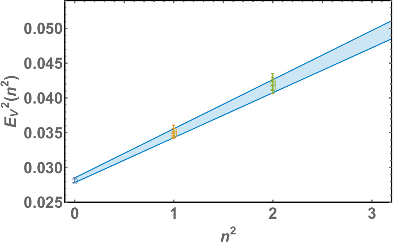 Figure 1
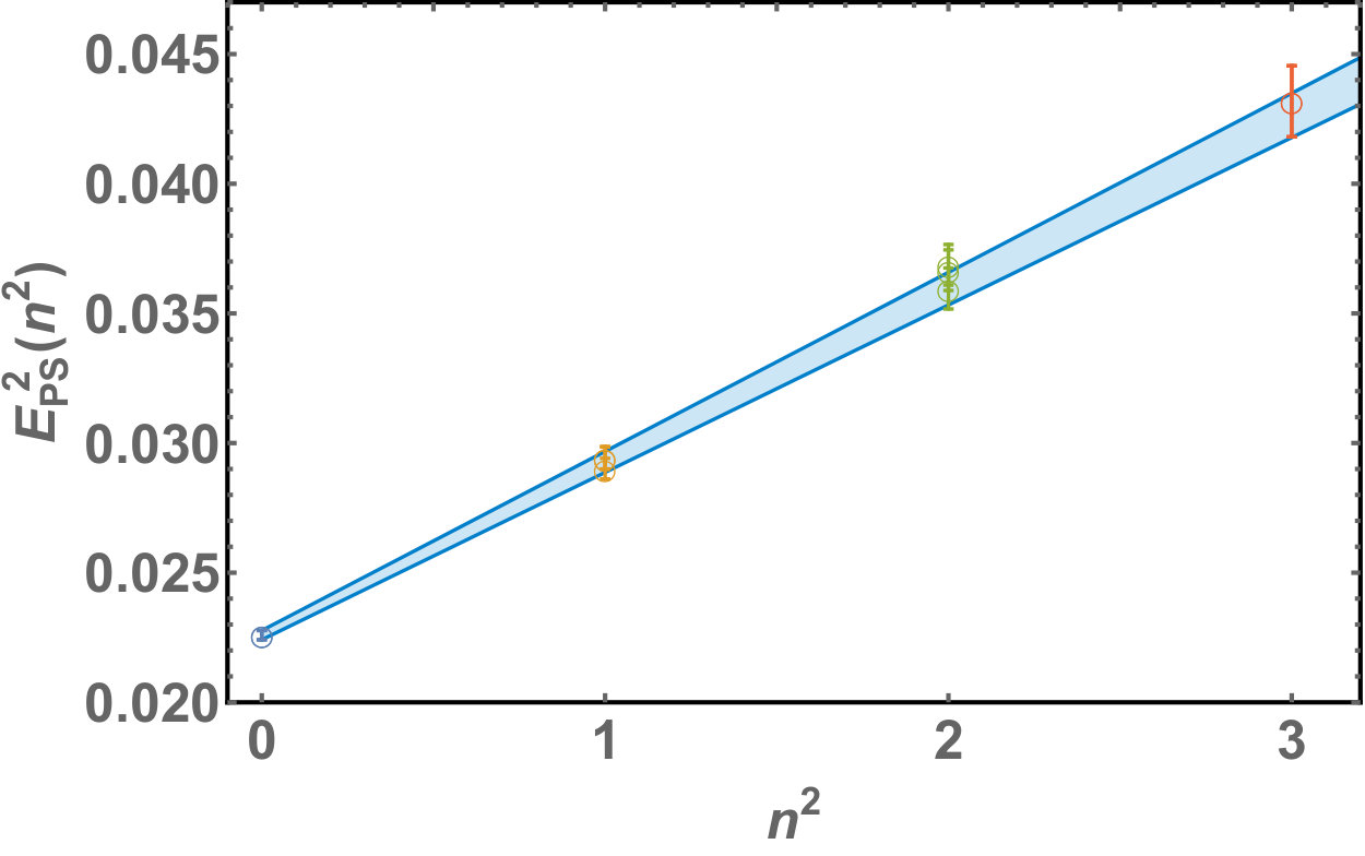 Figure 2
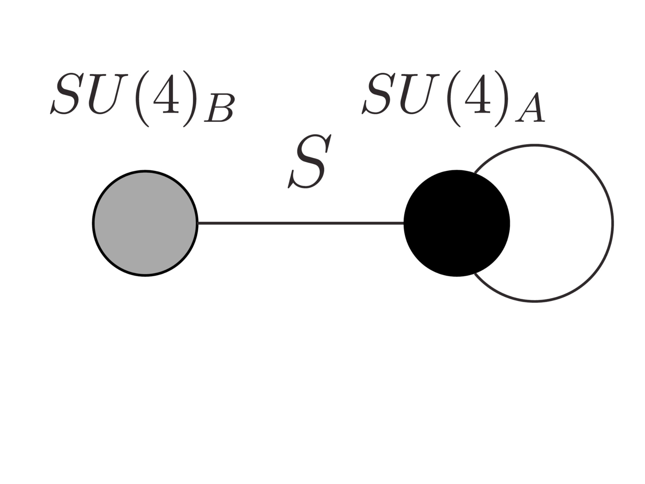 Figure 3
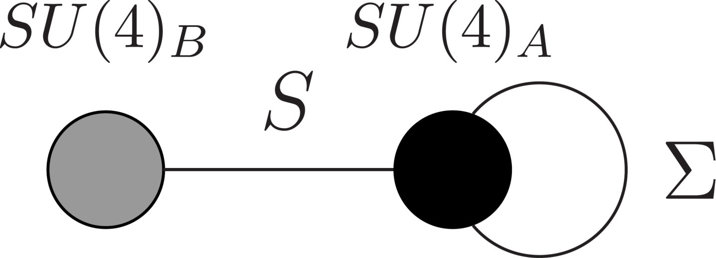 Figure 4
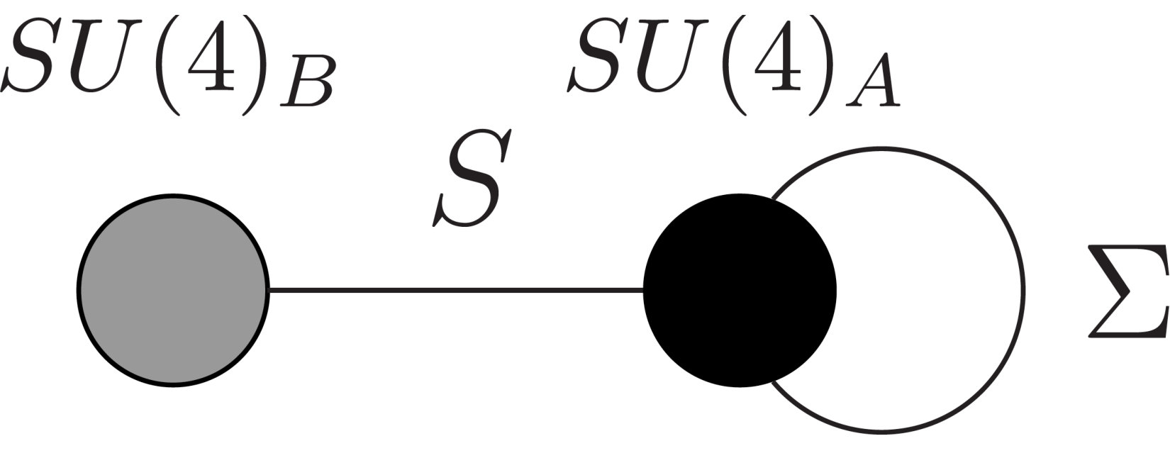 Figure 5
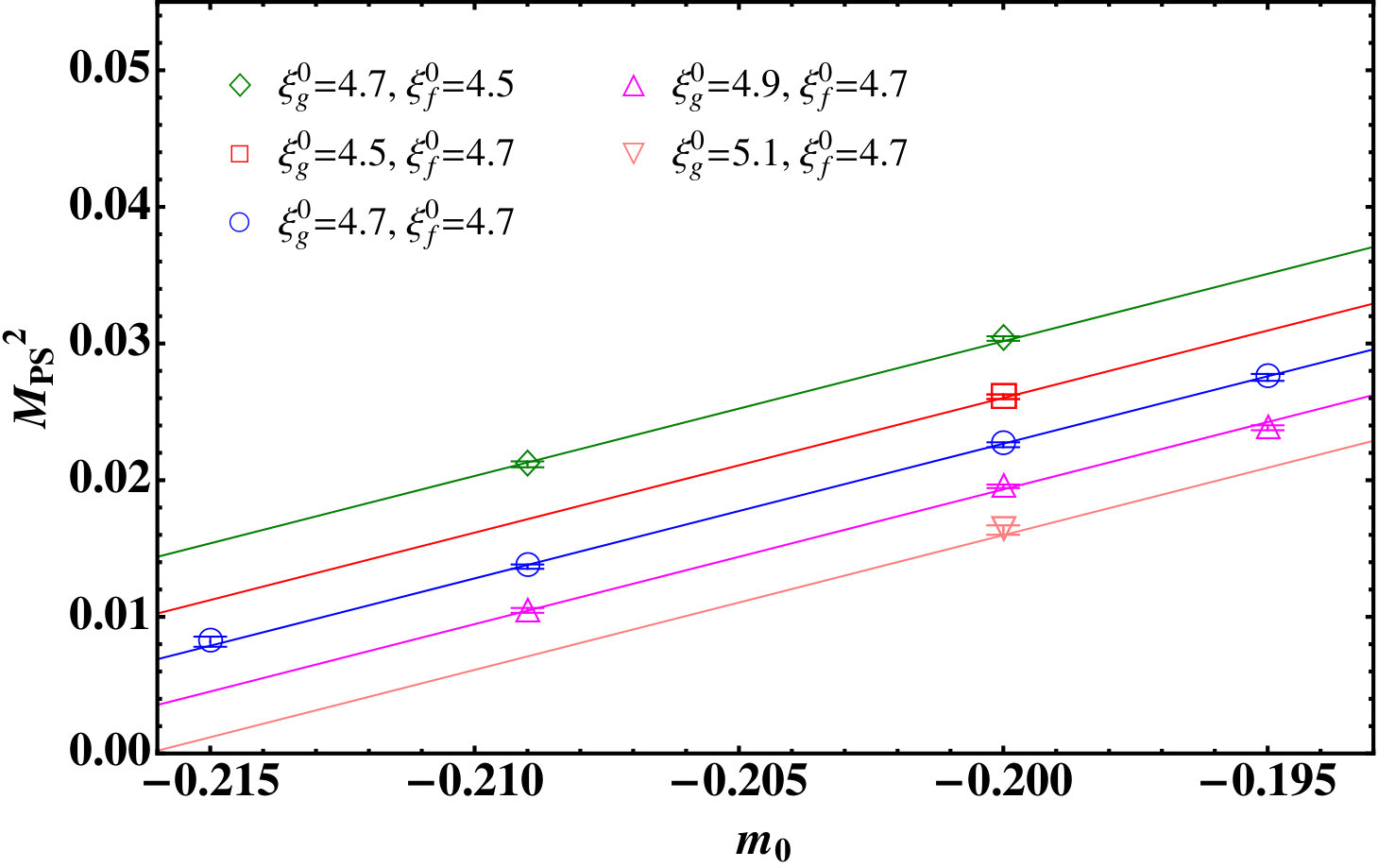 Figure 6
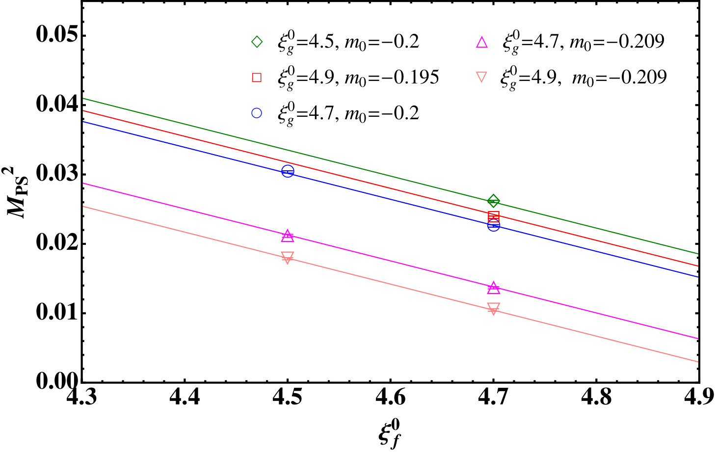 Figure 7
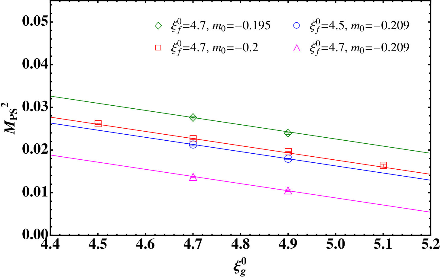 Figure 8
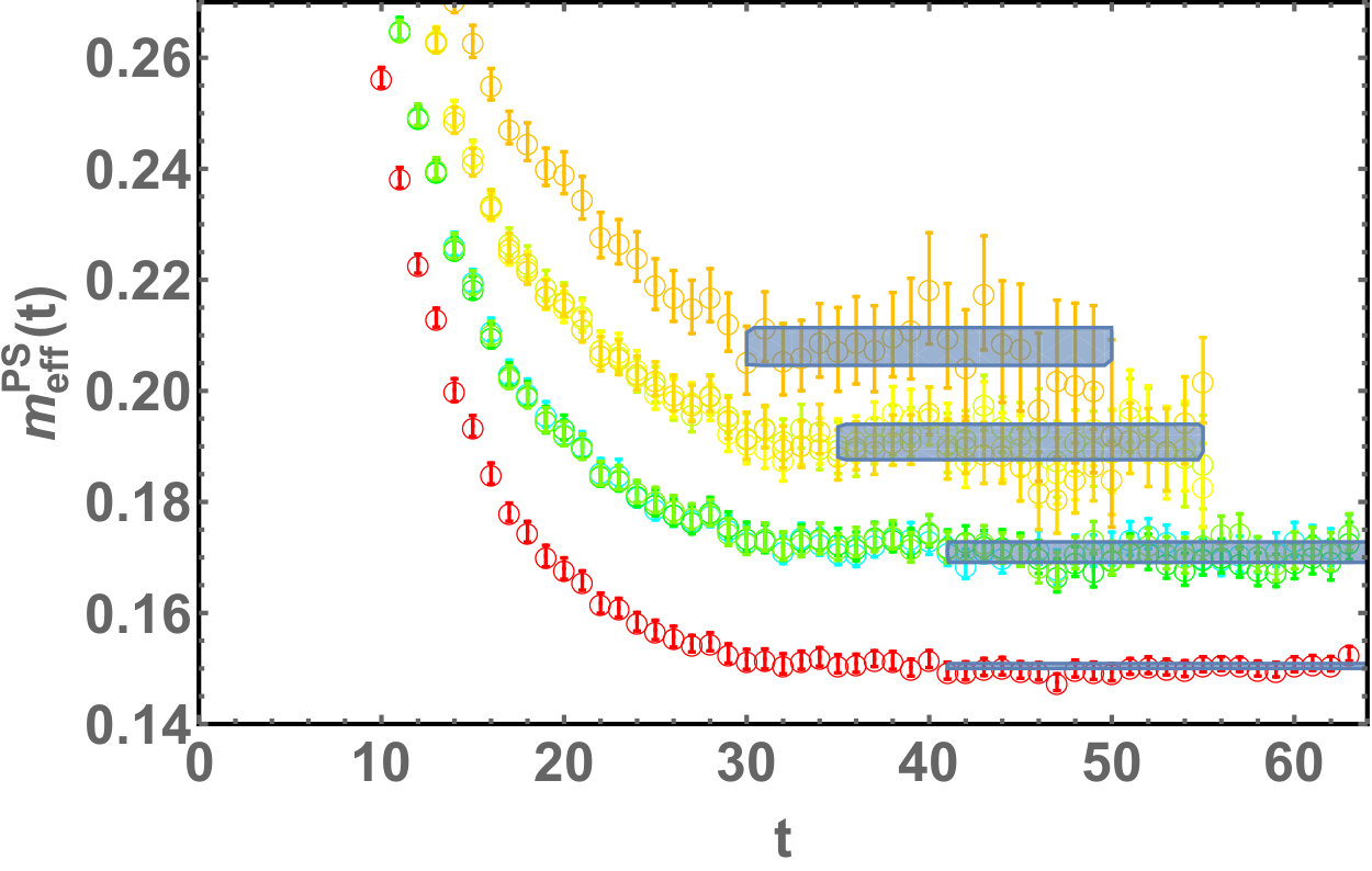 Figure 9
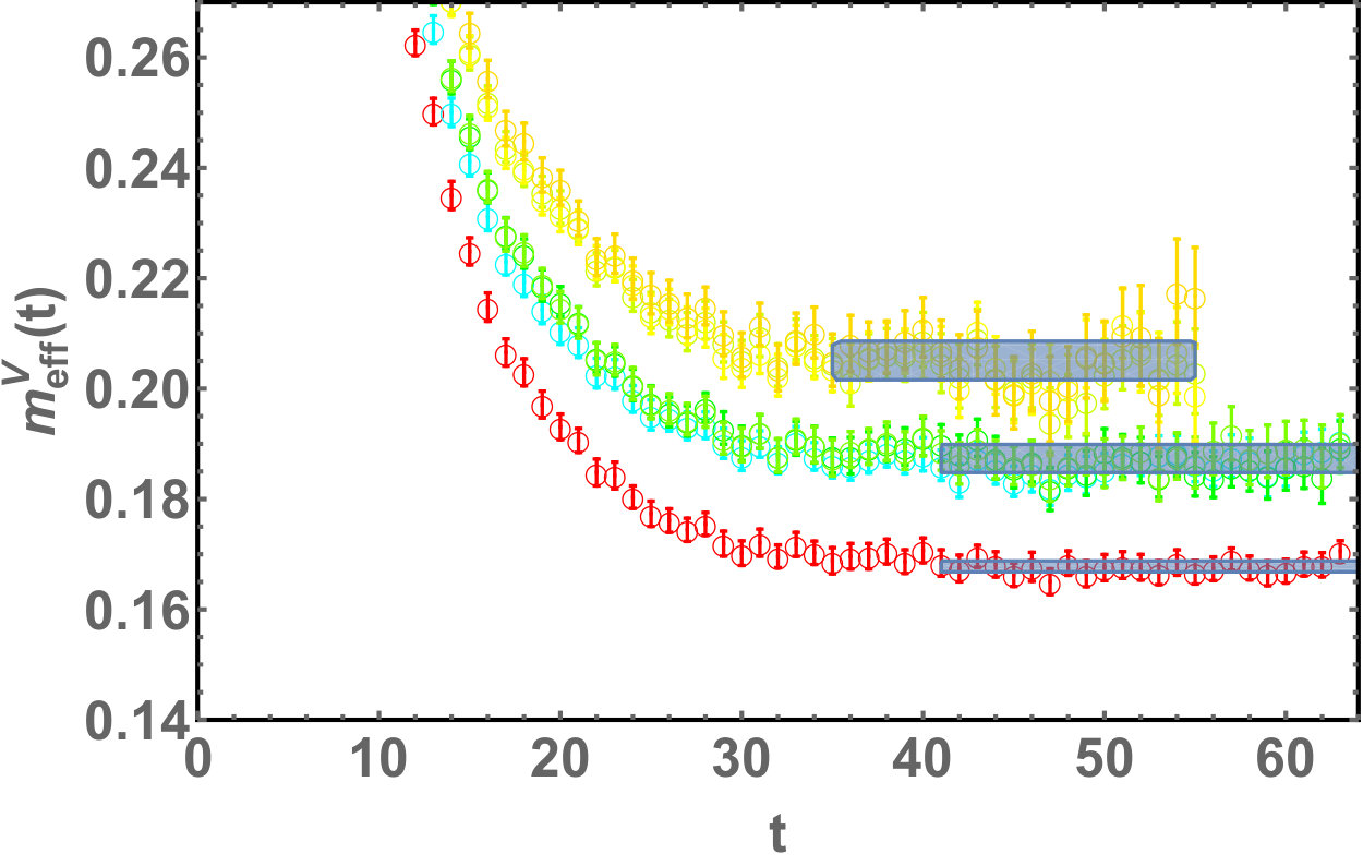 Figure 10
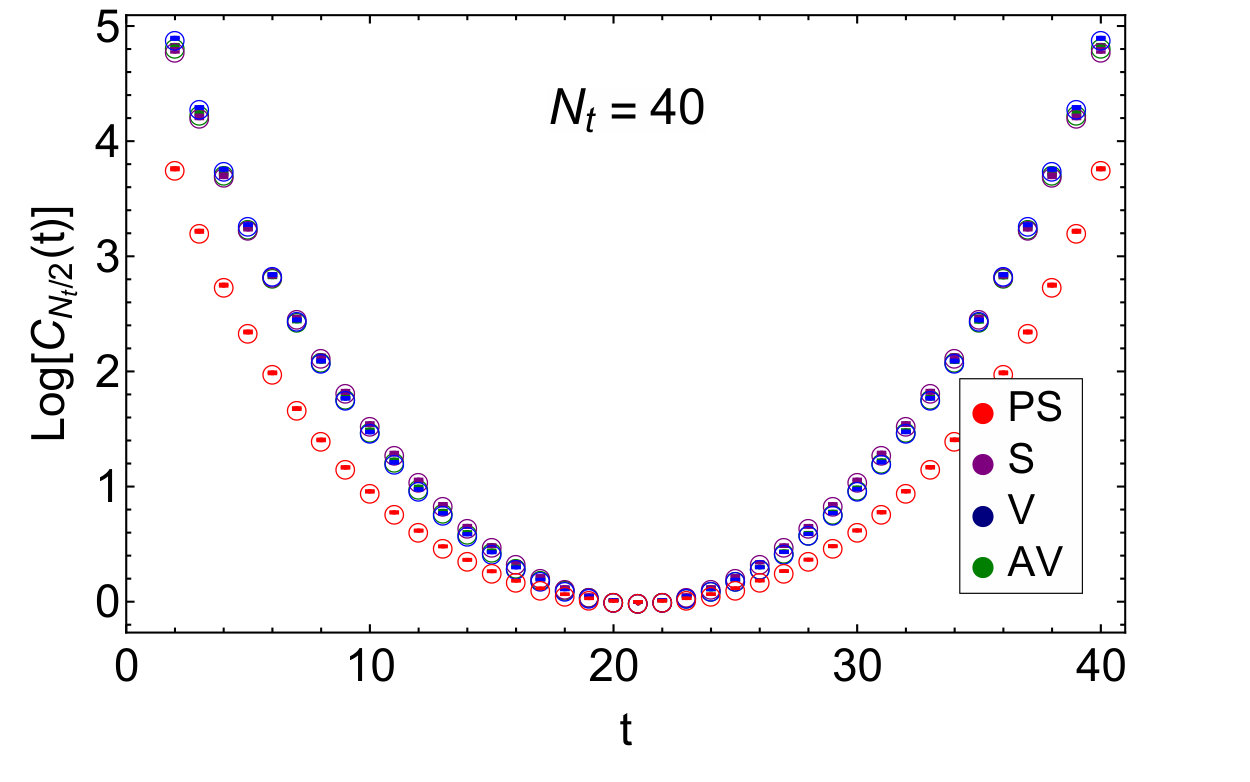 Figure 11
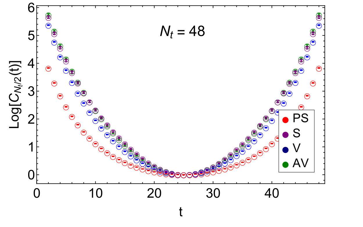 Figure 12
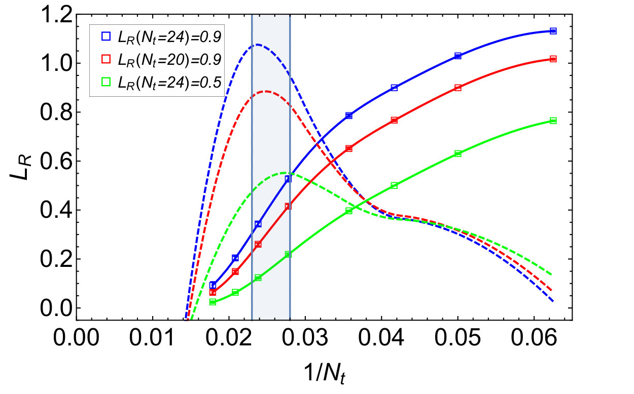 Figure 13
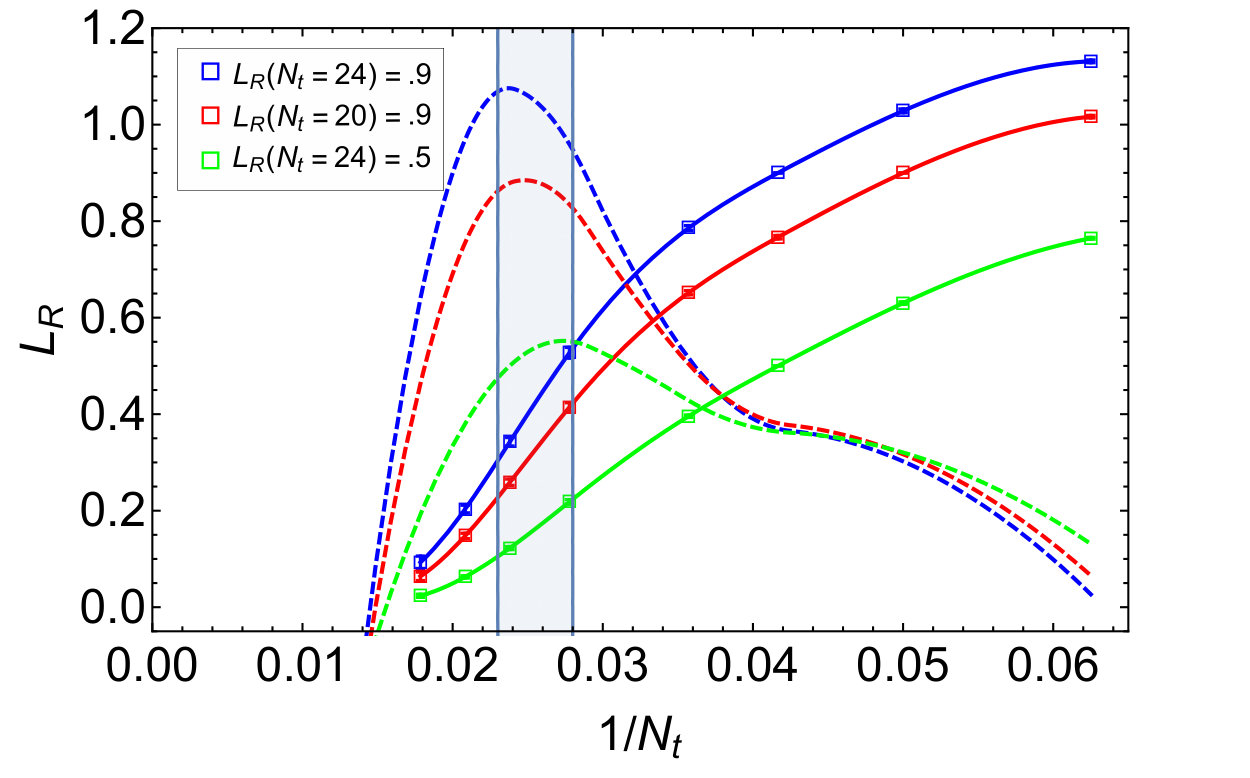 Figure 14
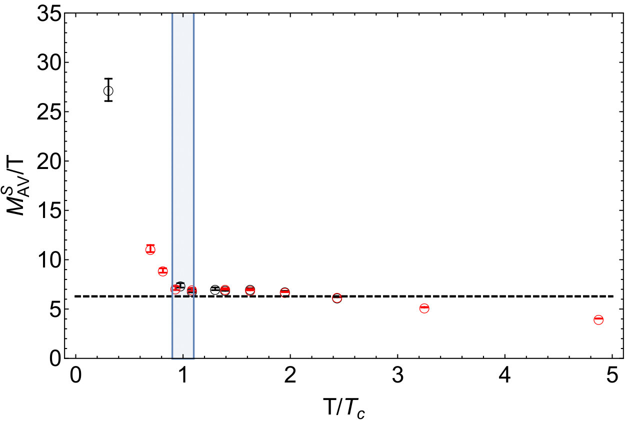 Figure 15
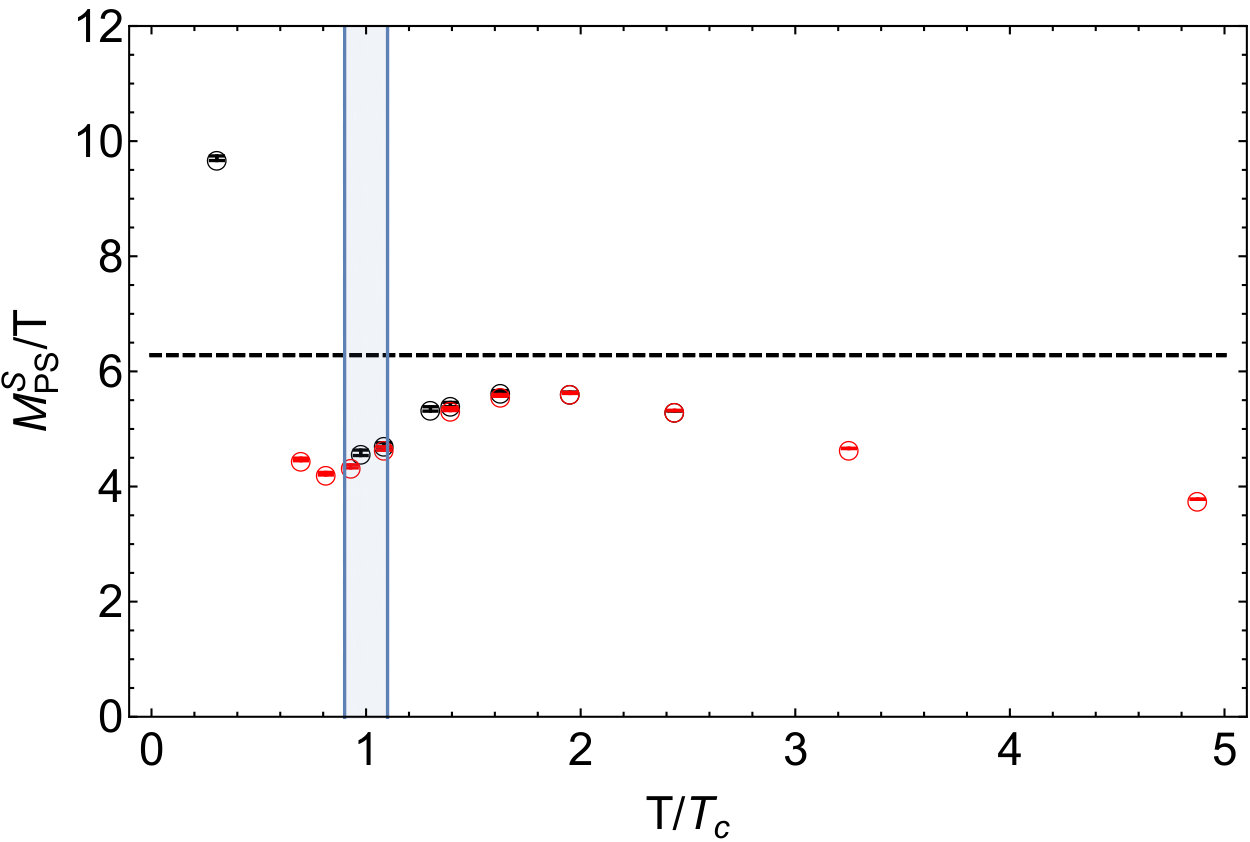 Figure 16
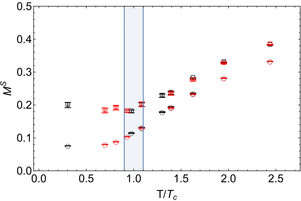 Figure 17
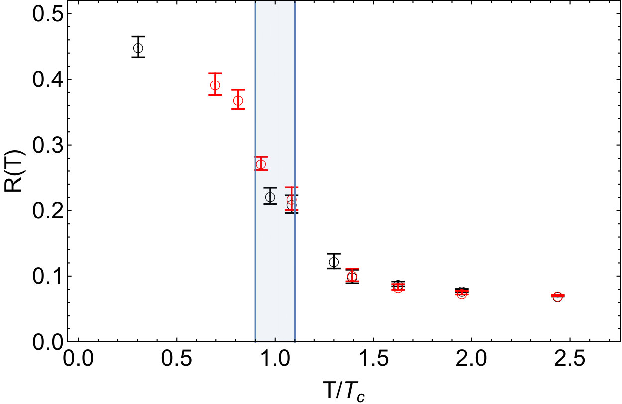 Figure 18
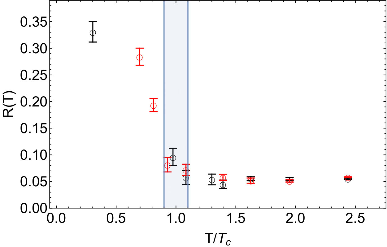 Figure 19
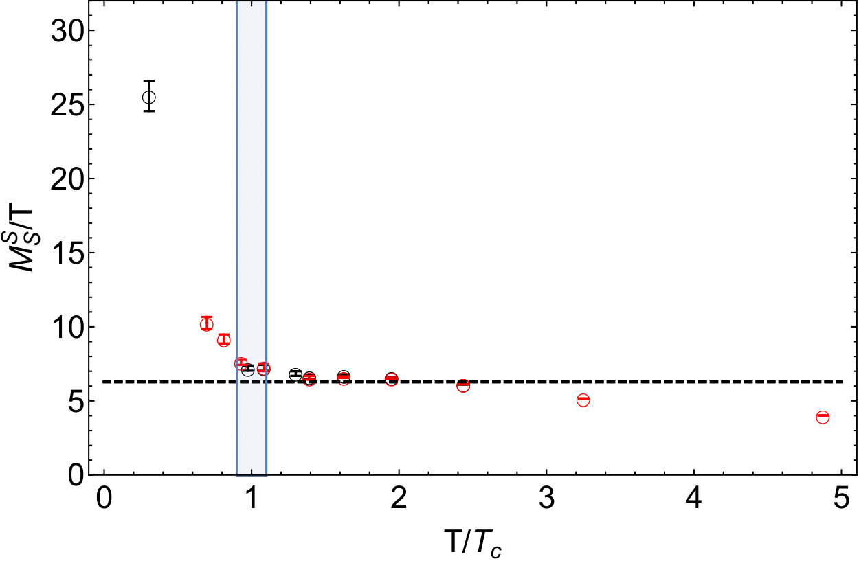 Figure 20
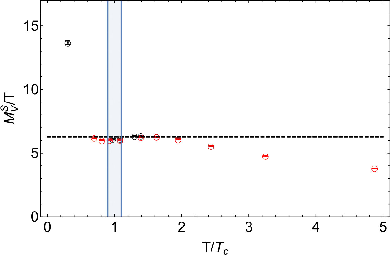 Figure 21
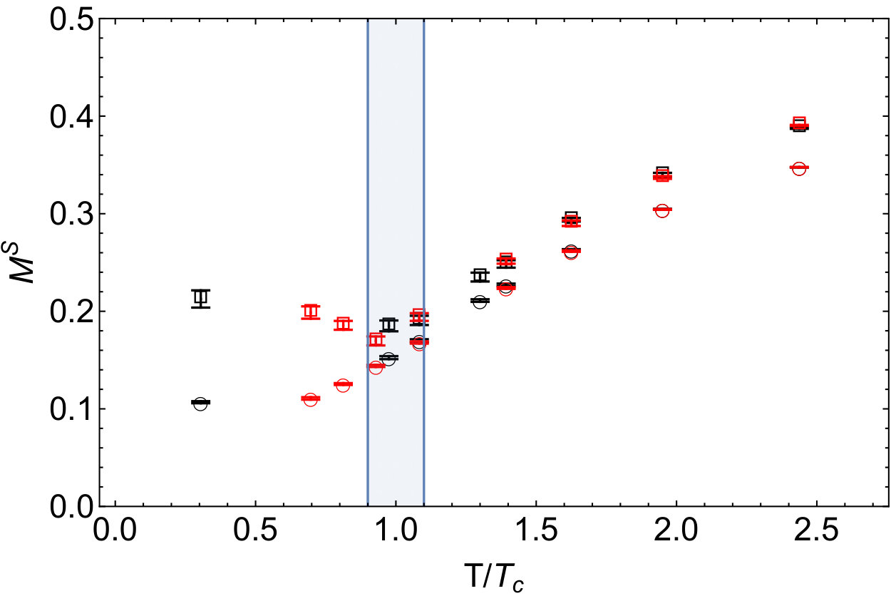 Figure 22
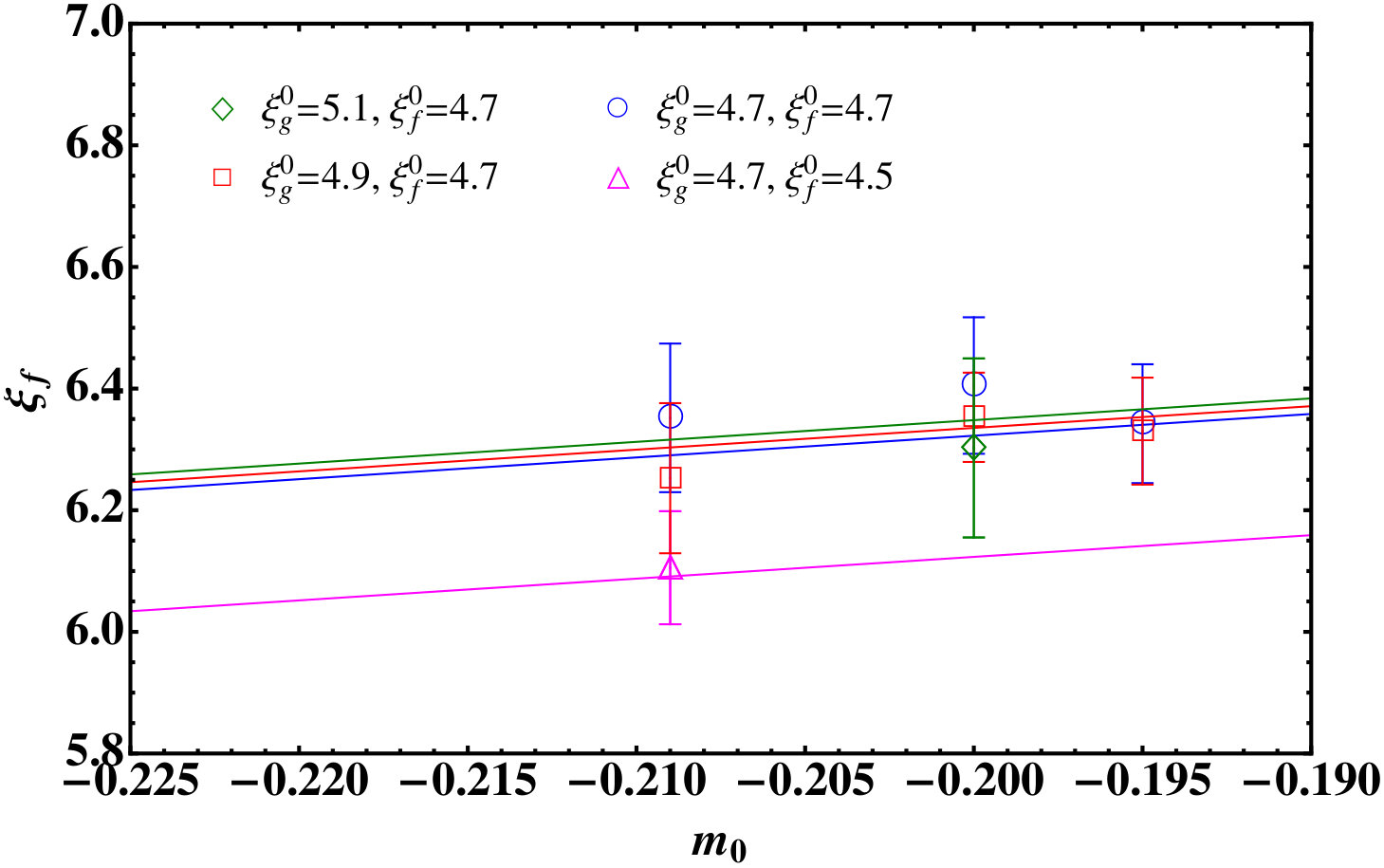 Figure 23
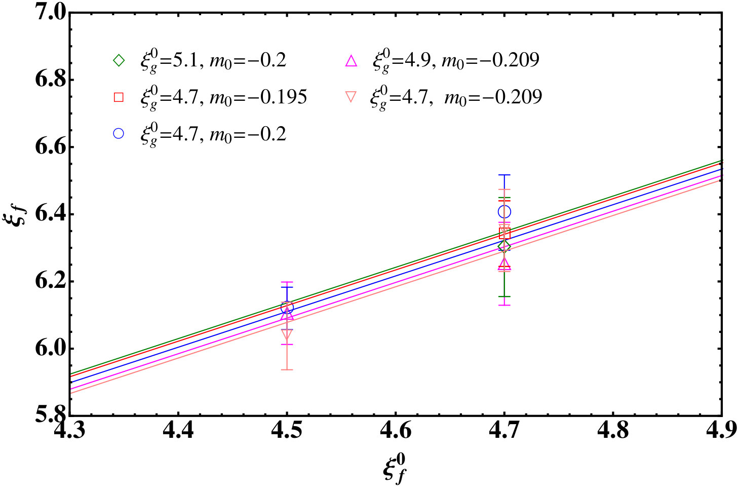 Figure 24
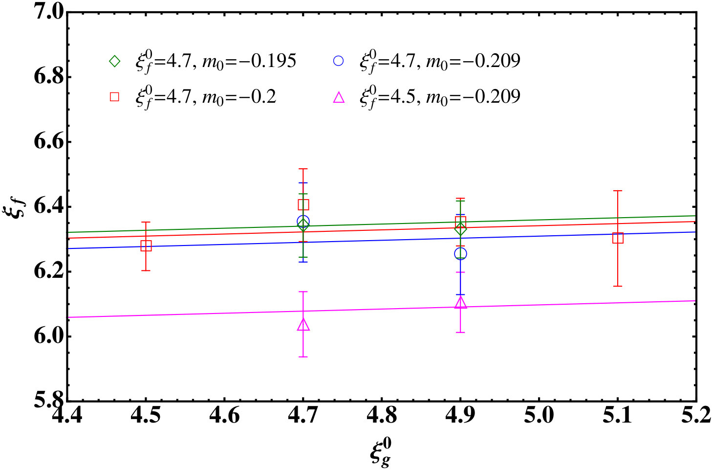 Figure 25
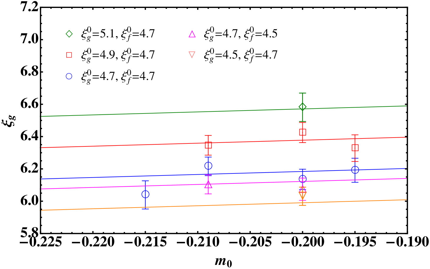 Figure 26
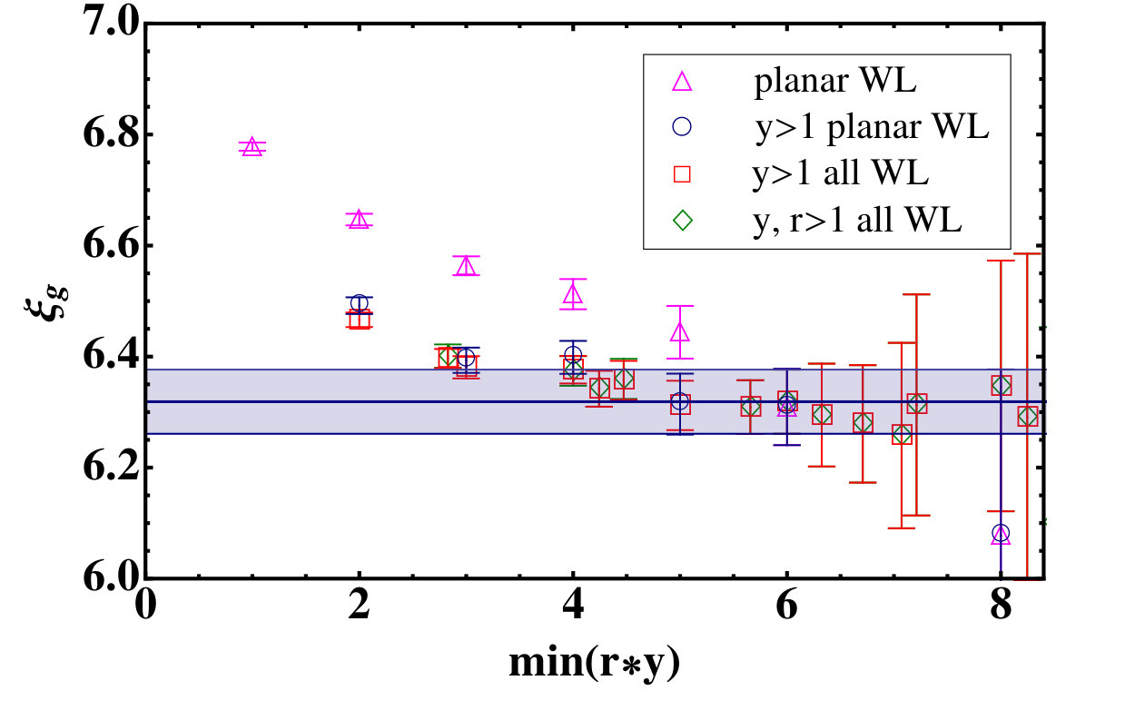 Figure 27
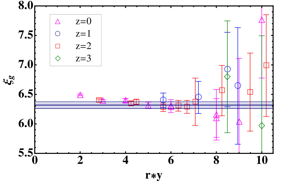 Figure 28
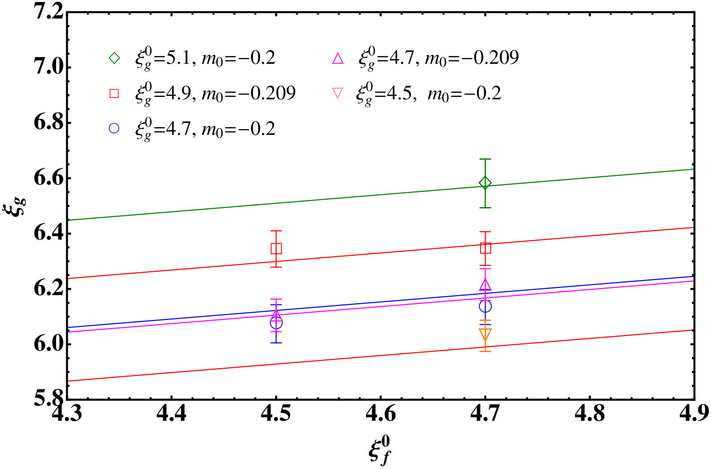 Figure 29
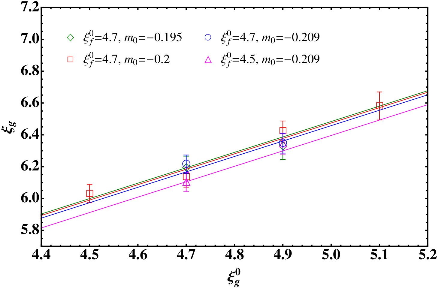 Figure 30
| Fields | ||
|---|---|---|
| -0.195 | 4.7 | 4.7 | 200 | 0.1659(8) | 0.1823(10) | 6.19(7) | 6.34(10) | 0.910(7) |
| -0.195 | 4.9 | 4.7 | 200 | 0.1544(6) | 0.1709(13) | 6.33(8) | 6.33(9) | 0.903(8) |
| -0.2 | 4.5 | 4.7 | 300 | 0.1616(5) | 0.1784(8) | 6.03(6) | 6.28(7) | 0.906(5) |
| -0.2 | 4.7 | 4.5 | 300 | 0.1743(5) | 0.1910(7) | 6.07(7) | 6.12(6) | 0.913(4) |
| -0.2 | 4.7 | 4.7 | 200 | 0.1504(6) | 0.1678(10) | 6.13(6) | 6.41(11) | 0.896(6) |
| -0.2 | 4.9 | 4.7 | 300 | 0.1399(5) | 0.1589(7) | 6.42(6) | 6.35(7) | 0.880(5) |
| -0.2 | 5.1 | 4.7 | 160 | 0.1279(13) | 0.1479(19) | 6.58(9) | 6.34(17) | 0.865(14) |
| -0.209 | 4.7 | 4.5 | 150 | 0.1455(7) | 0.1643(11) | 6.10(6) | 6.04(10) | 0.885(7) |
| -0.209 | 4.7 | 4.7 | 300 | 0.1169(7) | 0.1392(13) | 6.22(6) | 6.35(12) | 0.840(10) |
| -0.209 | 4.9 | 4.5 | 300 | 0.1336(6) | 0.1533(9) | 6.34(7) | 6.11(9) | 0.872(6) |
| -0.209 | 4.9 | 4.7 | 150 | 0.1023(9) | 0.1243(15) | 6.35(6) | 6.25(12) | 0.823(12) |
| -0.215 333 This ensemble is used only for the determination of and as the number of configurations is not large enough to determine in a reliable manner. | 4.7 | 4.7 | 138 | 0.0904(21) | 0.118(5) | 6.04(9) | 0.77(3) | |
| -0.209 444For this ensemble we carry out the measurements on the lattice. Note that . Compared to the lattice, we find no significant differences in all measured quantities. As for other ensembles, we therefore expect that the finite volume effects are negligible in the tuning of bare lattice parameters. | 4.7 | 4.7 | 300 | 0.1172(7) | 0.1382(11) | 6.13(6) | 6.42(13) |
| 16 | 16 | 2.44 | 200 | 24 | 8 | 4.88 | 200 |
|---|---|---|---|---|---|---|---|
| 20 | 1.95 | 200 | 12 | 3.25 | 200 | ||
| 24 | 1.63 | 200 | 16 | 2.44 | 225 | ||
| 28 | 1.39 | 200 | 20 | 1.95 | 150 | ||
| 30 | 1.30 | 200 | 24 | 1.63 | 200 | ||
| 36 | 1.08 | 200 | 28 | 1.39 | 250 | ||
| 40 | 0.98 | 200 | 36 | 1.08 | 380 | ||
| 128 | 0.30 | 215 | 42 | 0.93 | 388 | ||
| 48 | 0.81 | 390 | |||||
| 56 | 0.70 | 337 |
| 2.44 | 0.3322(2) | 0.3823(8) | 0.3475(2) | 0.3879(10) | 0.070(1) | 0.0549(13) |
| 1.95 | 0.2815(6) | 0.3292(14) | 0.3045(5) | 0.340(2) | 0.078(2) | 0.055(3) |
| 1.63 | 0.2355(6) | 0.281(2) | 0.2629(7) | 0.2938(18) | 0.088(4) | 0.056(3) |
| 1.39 | 0.1937(13) | 0.236(5) | 0.2272(12) | 0.248(4) | 0.099(10) | 0.045(8) |
| 1.30 | 0.1783(13) | 0.228(5) | 0.2110(13) | 0.235(5) | 0.123(11) | 0.054(10) |
| 1.08 | 0.1312(11) | 0.201(6) | 0.1699(15) | 0.191(5) | 0.210(13) | 0.057(13) |
| 0.98 | 0.1147(12) | 0.180(4) | 0.1525(16) | 0.185(6) | 0.222(12) | 0.096(16) |
| 0.30 | 0.0758(3) | 0.200(8) | 0.1068(11) | 0.213(9) | 0.449(16) | 0.331(19) |
| 4.88 | 0.4724(2) | 0.5021(8) | 0.4770(2) | 0.5044(7) | 0.0305(9) | 0.0279(8) |
| 3.25 | 0.3885(2) | 0.4293(15) | 0.3975(3) | 0.432(2) | 0.0498(18) | 0.041(2) |
| 2.44 | 0.33257(17) | 0.3833(8) | 0.34760(18) | 0.3905(5) | 0.0709(11) | 0.0581(7) |
| 1.95 | 0.2813(5) | 0.3268(15) | 0.3043(4) | 0.3371(14) | 0.075(3) | 0.051(2) |
| 1.63 | 0.2326(7) | 0.275(2) | 0.2617(7) | 0.290(3) | 0.083(4) | 0.052(5) |
| 1.39 | 0.1909(9) | 0.234(4) | 0.2239(9) | 0.251(3) | 0.102(10) | 0.058(6) |
| 1.08 | 0.1295(9) | 0.202(7) | 0.1680(11) | 0.194(4) | 0.218(17) | 0.072(11) |
| 0.93 | 0.1036(6) | 0.181(4) | 0.1440(11) | 0.170(5) | 0.272(10) | 0.081(13) |
| 0.81 | 0.0880(5) | 0.191(6) | 0.1254(9) | 0.186(5) | 0.369(15) | 0.193(12) |
| 0.70 | 0.0798(4) | 0.183(7) | 0.1107(13) | 0.199(6) | 0.393(17) | 0.284(16) |
Peer Reviews
No public reviews on file for this paper yet. If you reviewed it on a platform where reviews are public (OpenReview, ICLR, NeurIPS, ICML), you can paste yours below so the community can read it here.
Videos
No videos yet. Explain this paper in a talk, walkthrough, or lecture? Add one.
aainstitutetext: Department of Physics, College of Science, Swansea University, Singleton Park, SA2 8PP, Swansea, Wales, UKbbinstitutetext: Department of Physics, Pusan National University, Busan 46241, Koreaccinstitutetext: Extreme Physics Institute, Pusan National University, Busan 46241, Korea
Symmetry restoration at high-temperature in two-color and two-flavor lattice gauge theories
Jong-Wan Lee a
Biagio Lucini a
Maurizio Piai
Abstract
We consider the gauge theory with flavors of Dirac fundamental fermions. We study the high-temperature behavior of the spectra of mesons, discretizing the theory on anisotropic lattices, and measuring the two-point correlation functions in the temporal direction as well as screening masses in various channels. We identify the (pseudo-)critical temperature as the temperature at which the susceptibility associated with the Polyakov loop has a maximum. At high temperature both the spin-1 and spin-0 sectors of the light meson spectra exhibit enhanced symmetry properties, indicating the restoration of both the global and the axial symmetries of the model.
1 Introduction
We consider the gauge theory with flavors of Dirac fundamental fermions, and study the finite-temperature behavior by using numerical methods based on formulating the theory on anisotropic lattices. The main purpose of this work is to collect evidence that the global symmetries of the model are implemented à la Wigner at high-temperature, where the condensate breaking global symmetry is expected to melt and the global symmetries to be linearly realized.
This model has been considered before in three different contexts, as it represents the prototype of non-trivial gauge theory in which lattice numerical methods have concrete potential to provide useful information about the dynamics of the underlying theory. First of all, it is a useful toy model for the study of generalizations of Quantum Chromo-Dynamics (QCD) at finite temperature and finite chemical potential . One trivial reason for this is that the number of fundamental degrees of freedom is smaller than for two-flavor QCD, making the numerical treatment easier. Most importantly though, the fundamental representation of is pseudo-real, and hence there is no sign problem. It is then possible to study the phase diagram of the model in the -plane, and to apply numerical techniques to extract its detailed structure. For an incomplete list of useful references on the subject see LatticeSU2 .
A second context in which this model is important is that of traditional technicolor (TC) TC ; TCreviews . The choice of with fundamental Dirac fermions yields the minimal model such that one can embed the electro-weak group of the Standard Model of particle physics (SM) within the global symmetries of the matter field content. One expects spontaneous symmetry breaking to arise dynamically at the scale , hence providing a natural way to implement the Higgs mechanism for giving mass to the electroweak bosons within a fundamental theory. Aside from the fact that, once more, the small number of degrees of freedom makes practical applications amenable to numerical treatment, the fact that the field content is minimal also minimizes the potentially problematic contributions to precision parameters such as the oblique and as defined by Peskin and Takeuchi PT , that on the basis of perturbative arguments one expects to grow with and , and that are not dynamically suppressed when one identifies with the electroweak scale GeV. The dynamics preserves a custodial that further suppresses the parameter, as the underlying masses of the fermions vanish.
The model has received some attention in a third context sannino ; SU4Sp4 , as a concrete realization of the idea of Higgs compositeness compositeness . This is a quite distinct framework in respect to traditional TC. The underlying dynamics is the same, being based upon a gauge theory with a given global symmetry, for which one expects the formation of a non-trivial symmetry-breaking condensate. Yet, one chooses to embed the electroweak gauge group into the global symmetry group of the theory in such a way that the fermion condensate does not break it. 111We ignore the problem of vacuum alignment Peskin . The long-distance behavior of the theory is hence captured by an Effective Field Theory (EFT) that includes the SM gauge theory, supplemented by a set of light, composite pseudo-Goldstone bosons arising at the scale , a subset of which is interpreted as the Higgs doublet field.
The gauging of the SM group explicitly breaks the global symmetries, and hence provides a potential for the Higgs fields. Additional ingredients, not arising from the fundamental gauge theory, are invoked in order to drive spontaneous symmetry breaking in the Higgs sector, which ultimately yields electro-weak symmetry breaking (EWSB) at the scale . For example, one has to introduce a mechanism to give mass to the SM fermions, which requires coupling the Higgs field to the quarks and leptons. It is well known that, as a byproduct of doing so, the theory yields radiative corrections to the Higgs potential due to loops of the top quark, naive estimates of which show that they can destabilize the minimum of the Higgs potential. In the following we will not discuss any of these points, related to realistic model-building in the electro-weak sector.
The reason why composite scenarios are viable within this model originates from the pseudo-real nature of the fundamental representation of . In particular, in the presence of two Dirac fermions, the global symmetry of the Lagrangian is enhanced from the global symmetry of QCD and TC to a global symmetry, and the condensate breaks it to the subgroup. Excluding for the time being the anomalous from the discussion, this yields (pseudo-)Goldstone bosons, that form a multiplet of the unbroken . The gauging of splits the into a of , which is identified with the Higgs doublet, and an additional singlet, that may have important phenomenological implications.
In this paper, we compute the masses of the composite (meson) states created and annihilated by operators of the form , with , and discuss their dependence on temperature . 222 We refer the reader to the works in LatticeSU3Quenched ; Cheng ; LatticeSU3 : while these papers study gauge theory, some of their results and ideas play a role in the present paper.
In particular we track how the mass-splittings between parity partners change by going to high-temperature. In order to do so, we formulate the theory on anisotropic lattices, and use Monte Carlo methods to extract the spectral masses as a function of . We are looking for clear signals of the restoration in the thermal bath of the much larger global symmetry of the underlying theory. This is the first step of a more ambitious and long-term program, which we envision will include also the study of the effects due to the presence of explicit symmetry-breaking terms, in particular due to the chemical potential , and to the weakly-coupled gauging of the SM electroweak group.
The paper is organized as follows. In Section 2 we describe the model and summarize effective field theory and symmetry arguments that play a role in the rest of the paper. In Section 3 we describe the lattice set-up used in the numerical calculations, particularly by explaining in details how the bare parameters are tuned in the presence of anisotropic lattices. In Section 4 we report our results, which we critically discuss in Section 5. Appendix A contains some useful notation about spinors, and we show explicitly how the enhanced global symmetry emerges. In Appendix B we summarize the algebraic properties of and , by providing an explicit example of generators for . Examples of the renormalized versus bare parameters are given in Appendix C.
2 The model: symmetry considerations
The matter field content consists of two (massive) Dirac fermions , where is the color index and the flavor index. The covariant derivative is
[TABLE]
with the gauge fields, the coupling, and the generators of obeying , so that . The Lagrangian density is
[TABLE]
where the summations over flavor index and color index are understood, and where the field-strength tensors are defined in terms of the gauge bosons as .
We collect in Appendix A and B several useful relations between 2-component spinors and 4-component spinors , as well as details about the algebra of and (see also sannino ; SU4Sp4 ). The global symmetry acting on the matter fields is , and we explicitly list the transformation properties of the fields in Table 1. It is convenient to define:
[TABLE]
and to write the mass explicitly as a matrix , with the symplectic matrix in Eq. (74). The index and acts on spinor indexes. In the lower half of Table 1 we list the transformation properties of the composite field , as well as the (symmetry-breaking) spurion .
In the body of the paper, we will describe the finite-temperature properties of composite states that we identify with the pions , vector, axial-vector, and scalar mesons. In the rest of this Section, we summarize the basic properties of these objects, using the language of effective field theory (EFT). What results is a Lagrangian density that includes potentially heavy and strongly-coupled degrees of freedom, and hence does not yield a calculable weakly-coupled low-energy EFT in the usual sense. We use this language to guide our book-keeping exercise, focused on classifying the physical particles, their quantum numbers, and the degeneracies—in particular the difference of mass between the and vectors and between the and scalars— that are consequences only of the symmetry structure of the theory and its vacuum.
2.1 Composite states: scalars
In the low-energy EFT description, the real antisymmetric field transforms as
[TABLE]
under the action of an element of . The VEV breaks to the subgroup. The generators with are broken, while with are unbroken. For instance, see Eq. (89) in Appendix B.
In terms of the matrix-valued , the convenient parameterization
[TABLE]
automatically satisfies the non-linear constraint . The leading-order term of the low-energy EFT is
[TABLE]
The pion fields are canonically normalized and hence is the pion decay constant.
The quark mass is incorporated in the EFT by adding the symmetry-breaking term
[TABLE]
The expansion in pion fields confirms that the pions are still degenerate, if not massless, in the presence of the explicit breaking given by the Dirac mass for the fermions, with
[TABLE]
The degeneracy of the five pions is a consequence of the unbroken symmetry. The spurion formally transforms as , so that if it were promoted to a field then would be manifestly invariant under the full symmetry.
Here we pause to make two general observations. In the context of composite-Higgs models, the presence of a (small) mass term for the quarks is allowed, contrary to the TC case. While in the latter the quark mass explicitly breaks the gauge symmetries, in the composite-Higgs case the SM gauge group is a subgroup of , and hence the term in Eq. (8) does not break it. The distinction between TC and composite-Higgs cases reduces (in the massless case) to a vacuum alignment issue driven by the weak gauging of the symmetry. In the presence of a mass of the form in Eq. (8), this problem has a trivial solution: the mass stabilizes the composite-Higgs vacuum. Yet, some caution is in order: if is large, it might become impossible to induce electro-weak symmetry breaking. We leave these and similar issue out of this study (see VA ), as in our numerical work all calculations are done with the theory in isolation.
To describe the regime in which the symmetry is restored, which is expected to be realized at high temperature, we remove the non-linear constraint, and hence replace by the field , that transforms as a complete antisymmetric representation of . The kinetic term is
[TABLE]
The Lagrangian density contains a potential as any arbitrary function is allowed by the symmetries. The minimization of yields the identification . The small fluctuations of are parameterized in terms of the pion fields along the broken directions, plus an additional real scalar :
[TABLE]
where the normalizations are chosen so that all the fields have canonical kinetic terms. Unconstrained by symmetry considerations, the scalar (singlet of ) is expected to have a large mass , and in general decay fast to pions.
Besides the breaking, the vacuum also induces the breaking of the (anomalous) . To discuss it, we need to promote a complex field, hence doubling the field content. We define
[TABLE]
with a second real antisymmetric representation of . The action of is
[TABLE]
where is the parameter of the transformation. The field introduces an additional singlet that is the analog of the in QCD and additional scalars that form a multiplet of the unbroken symmetry, and are the analogue of the isovectors of QCD. The treatment presented here is indeed a generalization of what done in the context of the linear-sigma-model description of low-energy QCD LSM .
The presence of the anomaly produces a large mass for . At high temperatures both the fermion condensate and the effect of the anomaly are suppressed. Hence, the mass splitting between and provides a measure of the level of breaking of in addition to global , and can be used to look for thermal restoration. Similar arguments hold in the case of QCD (see for example SU3a0 ; SU3eta and references therein).
Because the and are flavor singlets, and the flavor-singlet sector of the spectrum is more difficult to study numerically than the flavored channels, we will study the - mass splitting in order to discuss the restoration of the axial at high temperatures. We will do so in the body of the paper, using numerical techniques based on the formulation of the theory on anisotropic lattices.
2.2 Composite states: vectors
The full set of spin-1 vector and axial-vector mesons spans the adjoint representation of the global symmetry. A cartoon representing the EFT description of their long-distance dynamics is depicted in Fig. 1, and represents a generalization of hidden local symmetry HLS ; HLS2 ; HLS3 . One extends the symmetry from to , with weakly gauged, with coupling . Then one enlarges the field content to include two non-linear sigma-model fields and . The non-linear sigma-model transforms as the bifundamental of , while the field transforms on the antisymmetric of :
[TABLE]
In a composite-Higgs model, the SM gauge group is a subgroup of .
The gauging of the symmetry means that (for global ) one has to introduce the covariant derivatives
[TABLE]
and then is replaced by all possible 2-derivative invariant operators made by , , , , together with the kinetic term for the gauge bosons. Both and are non-vanishing in the vacuum, inducing the symmetry breaking pattern , and all vectors are massive. splits the mass of the and the mesons.
In unitary gauge, besides the heavy vectors only the physical pions are retained. They are linear combinations of the fluctuations of and . The mass term for the pions is
[TABLE]
The quark masses also contribute to the masses of the spin-1 states in a more complicated way, that will be discussed elsewhere elsewhere .
In the absence of the antisymmetric condensate (for ), and mesons would be exactly degenerate. Their mass splitting is hence a measure of the amount of breaking . In the main body of the paper we use the mass splitting between (vector) and (axial-vector) as a way to test whether the global symmetry is restored at high temperatures. The generalization to the case in which is replaced by does not require any new ingredients. In particular the restoration of the axial and of the global can, at least in principle, be treated independently. We summarize in Table 2 the properties of the states discussed in the body of the paper. One of the purposes of this paper is to make the first steps towards a quantitative assessment of the relation between the two phenomena at high temperature, in the specific theory of interest here.
3 Numerical results: Anisotropic lattice
3.1 Lattice action
In this Section, we describe the discretized Euclidean lattice action used for our numerical study. For the gauge sector, we modify the standard plaquette action by treating the operators containing temporal gauge links separately from those solely containing spatial links,
[TABLE]
where and are the lattice bare gauge coupling and the bare gauge anisotropy, respectively. The plaquette is defined by
[TABLE]
where denotes the link variables. For the fermion sector, we use the Wilson action for fermions in the fundamental represention
[TABLE]
with the massive Wilson-Dirac operator given by
[TABLE]
where and denote the forward and backward covariant derivatives, respectively:
[TABLE]
The ratio of the bare fermion to gauge anisotropy is introduced as it can be different to unity. From the redefinition of the fermion field ( and ), along with the introduction of the fermion anisotropy , we rewrite Eq. (21) as
[TABLE]
For the rest of this paper we do not explicitly show the lattice spacings for convenience, i.e. , except when we need to distinguish the spatial and temporal lattice spacings and to discuss the finite temperature.
The bare anisotropy parameters, and , are renormalized such that physical probes at scales well below the cut-off exhibit Euclidean symmetry, i.e. . For the input quark mass, , we parameterize the renormalized parameters as functions of bare parameters . For a small region in the parameter space, we assume that the renormalized parameters are linear in the bare parameters. We further assume that we are in the region of light quark masses, i.e. , and arrive at the form AnisoL
[TABLE]
For each set of bare parameters, nonperturbative determinations of and are carried out through the interquark potential and the relativistic meson dispersion relation, respectively, which will be discussed in details in the following subsections.
3.2 Simulation details
We consider the lattice action in Eq. (18) and Eq. (20) with two mass-degenerate Wilson fermions. Configurations are generated using the Hybrid Monte Carlo(HMC) algorithms with the second order Omelyan integrator for Molecular Dynamics(MD) evolution, where different lengths of MD time steps are used for gauge and fermion actions such that the acceptance rate is in the range of . The simulation codes are developed from the HiRep code HiRep modified by implementing the gauge and fermion anisotropies described in Section 3.1. To optimise the acceptance rate, we also treat the variance of temporal and spatial conjugate momenta differently by introducing a new tunable parameter MSU , which is essentially equivalent to the multiscale anisotropic molecular dynamics update AnisoL . Without changing the validity of the algorithm, such a setup is helpful for the anisotropic lattice calculations through balancing the temporal and spatial MD forces: typically the former is larger than the latter approximately by the anisotropy in the lattice spacings.
Except the lattice of for the investigation of finite volume effects, all of the numerical calculations for the tuning of bare parameters are performed on lattices. We use periodic boundary conditions in each direction of both link variables and fermion fields. 555 We have checked that using antipeoriodic boundary conditions in the time direction for fermions give compatible results as expected in zero-temperature calculations. Twelve ensembles are created with different bare quark masses, gauge and fermion anisotropies at , where the details are found in Table 3. Thermalization and autocorrelation times are estimated by monitoring the average plaquette expectation values. For each ensemble configurations are accumulated after trajectories for thermalization, where every two adjacent configurations are separated by one auto-correlation length of which the typical size is trajectories. The statistical errors for all quantities extracted in this work are obtained using the standard bootstrapping technique.
3.3 Gauge anisotropy
The gauge anisotropy is determined from the static potential using Klassen’s method Klassen . We first define the ratios of spatial-spatial and spatial-temporal Wilson loops by
[TABLE]
respectively. In an asymptotic region, these ratios fall exponentially with the linear interquark potential and do not depend on , and . Finite volume effects are expected to be suppressed since they are canceled out in the ratios Umeda ; Klassen . As the interquark potential at the same physical distance should yield the same value, one can extract the anisotropy by imposing . In practice, we determine by minimizing Umeda
[TABLE]
with
[TABLE]
where and are the statistical errors of and , respectively.
In the original Klassen’s approach, the planar Wilson loops are considered where is either or . A typical difficulty in this approach is the limited number of data points as one quickly encounters a severe signal-to-noise problem in the calculations of the large Wilson loops. By noting that can be any two-dimensional path in the - plane with , we extend the Klassen’s method by including nonplanar Wilson loops along the closed path and with . To maximize the overlap with the physical ground state the shortest paths in the - plane are considered using the Bresenham algorithm which has been applied for the lattice study of quark antiquark potential, i.e. see BA . Analogous to the planar case, we define and for a fixed value of .
Using the generalized Klassen’s method, we are able to secure enough data points having reasonable statistical errors. As a consequence, not only do we find the clean signal of an asymptotic region in which converges, but also reduce the statistical error of the gauge anisotropy . However, due to the breaking of rotational symmetry on the lattice, results obtained mixing on-axis and off-axis loops might be affected by a large systematics. To investigate this issue, we calculate by minimizing the function with , corresponding to the different shapes of the 2-dimensional paths. The results are shown in Fig. 2. We find no significant deviations between colored data, suggesting that any potential effect of the breaking of rotational symmetry cancels in the ratios of Wilson loops in Eq. (25). For all data points are statistically consistent with one another. The measured value of is denoted by the blue band in the figure, where its extraction is discussed in the following.
In Fig. 3 we plot , obtained by using Eq. (26), as a function of for four different sets of data: all planar Wilson loops (purple triangle), planar Wilson loops except (blue circle), planar and nonplanar Wilson loops except (red square), and planar and nonplanar Wilson loops except and (green diamond). The largest value of is the one before we encounter significant numerical noise.
For all ensembles we find that converges to the asymptotic value at around and thus we choose , as for this value we expect the size of systematic errors to be small compared to the statistical error. Since the inclusion of Wilson loops causes significant systematic effects due to short-range lattice artefacts, as can be seen in the plots (see also the discussion in Umeda ; AnisoL , in the case of QCD), we exclude these Wilson loops for the determination of . In summary, we calculate the asymptotic value of using planar and nonplanar Wilson loops, except the ones having , at and the results are reported in Table 3.
3.4 Fermion anisotropy
The fermion anisotropy is determined through the leading-order relativistic dispersion relation of mesons
[TABLE]
where is the spatial lattice size. The energy and the mass are in units of , while the momentum is in units of . In the Euclidean formulation, meson two-point correlation functions exponentially fall off with the lowest energy at an asymptotically large time. In practice, it is useful to define an effective mass,
[TABLE]
where is the ensemble average of meson correlators. Then, ground state energies are obtained from a constant fit to the plateau of in the asymptotic region of large . In the case of zero momentum these energies are nothing but the meson masses. The measured masses of pseudoscalar and vector mesons are reported in Table 3.
As an example, in Fig. 4 we show the effective mass plots for pseudoscalar and vector mesons with , and . We construct the meson interpolating operators at source and sink using point sources. Various momentum projections with are denoted by red, green, yellow and brown colors, respectively, while the measured ground state energies are denoted by the blue bands.
In Fig. 5 we plot the resulting squared energy as a function of and find a good linearity, consistent with Eq. (28). In the determination of , to minimize the systematic effects due to excited state contamination at higher momenta, we only use the lowest four momentum vectors in the linear fit of to Eq. (28). As seen in the figures, the fit results denoted by blue bands explain the data very well. The extracted value of from a pseudoscalar meson is in good agreement with the one from a vector meson, , and shows better precision. Therefore, for the tuning of lattice bare parameters we use from pseudoscalar mesons which are summarized in Table 3.
3.5 Tuning results
To determine the coefficients, , , and , we perform the simultaneous fit of the numerical data in Table 3 to the functions in Eq. (24). The results are
[TABLE]
where the values of per degrees of freedom are , , , respectively. In Appendix C we show some examples of the results of the fit in the two-dimensional spaces of the renormalized and bare parameters.
Our interpretation of the above results requires that we comment on a few important features. First of all, renormalized anisotropies are somewhat larger than the bare anisotropies, which we interpret as a signal of the fact that the calculations are performed far from the weak coupling limit. Secondly, we find that the coefficients and are small, in particular, is zero within the statistical errors. In the quenched approximation, one would expect that the gauge and fermion anisotropies can be determined independently. The mild dependences of on and on are consistent with the fact that this part of the numerical study is performed in the regime of heavy quarks. Yet, we note that over the range of considered lattice parameters our results show a good linear dependence of the squared mass of a pseudoscalar meson on the bare quark mass , which is consistent with our use of Eq. (24) to extrapolate to the limit of vanishing physical mass for the quarks.
In order to determine the values of the bare parameters at our chosen reference point we impose the following renormalization conditions:
[TABLE]
Solving Eq. (24) with our target renormalized parameters of and , we find
[TABLE]
We will use these choices for the lattice parameters in measuring the physical properties of the field theory. Note that falls slightly outside the range of masses used in this part of the study (see Table 3), and hence we expect some (small) residual quark mass and symmetry-breaking effects to be present in our physical simulations.
4 Numerical results: Finite temperature
From now on, the lattice bare parameters are fixed by the central values in Eq. (32) along with . We perform finite temperature calculations on the anisotropic lattices of and . Simulation details and numerical results for these two lattices are summarized in Tables 4, 5 and 6. Two different values of are considered to estimate the systematic errors due to excited state contaminations in the calculations of screening masses. The algorithms for the generation of gauge ensembles have been discussed in Sec. 3.2.
Before we discuss the numerical results of finite temperature calculations in details, we perform a zero temperature calculation in order to check how well the tuned bare parameters are working. Using the ensemble of in Table 5, we obtain , , and . These results are compatible with the renormalized parameters of and , where the largest uncertainty occurs in the detemination of with . Finite volume effects are expected to be negligible as the lattice volume is much larger than the size of the pseudo-scalar meson, .
Adopting anti-periodic boundary condition along the temporal direction, temperature is defined by . We will find it convenient to measure the temperature in units of the (pseudo-)critical temperature , discussed and measured in the next section.
4.1 Deconfinement crossover
As is the case for QCD with small number of quarks, our model is also expected to exhibit confinement at low temperature and form a quark-gluon plasma across the (pseudo-)critical temperature . Although the Polyakov loop is not an exact order parameter when the number of quarks is finite, it is widely used as an indicator of deconfinement. Following the method used in RPM1 ; RPM2 , we define the expectation value of the renormalized Polyakov loop666 For the discussion of the renormalized Polaykov loop and its scheme dependence, we refer the reader to RPM3 ; RPM4 . by
[TABLE]
where the bare Polyakov loop is related to the bare free energy as . The multiplicative renormaliztion constant is defined by , which only captures the short distant physics and thus is independent on the temperature. As different choices of denote different renormalization schemes, to incorporate the scheme dependence on the detemination of we impose a renormalization condition for a given temperature by .
We consider three renormalization schemes, defined by the conditions , , and respectively. The results are shown in Fig. 6. The temperature is determined from the peak of the susceptibility of the Polyakov loop, , denoted by dashed lines in the figure. Combining the statistical uncertainty and the systematic uncertainty of scheme dependences in quadrature, we find that , or equivalently that . As anticipated, we will measure temperatures in units of this in the following.
4.2 Temporal correlation functions
At zero temperature, the Euclidean two-point correlation functions of mesonic observables fall off with a single exponential at a large time so that the ground state energy of mesons can be extracted in a clear way in principle. In the finite temperature lattice calculations this process is affected by some limitations. Firstly, the maximum available physical temporal extent is limited by the inverse of the temperature. In addition, a single exponential analysis becomes subtle as the spectral function of mesons no longer exhibits a sharp peak at the mass of mesons. In this case, it is more desirable to investigate the correlation functions by themselves.
We introduce the normalized correlation function with the reference choice :
[TABLE]
We consider isovector pseudo-scalar, scalar, vector, and axial-vector mesons, where the corresponding interpolating fields are defined by
[TABLE]
respectively (flavour indices selecting non-singlet states are understood). In order to improve the statistics, we use stochastic wall sources SWS for the study of meson spectrum at finite temperature. Using these mesonic operators we compute the function . In Fig. 7 we show the results of for and , which exemplify the typical behaviors of below and near respectively.
By comparing the two plots in Fig. 7 one can see that while at low temperature () the vector and axial-vector correlators are different, they become hard to distinguish from one another in proximity of (). The overlap of between vector and axial-vector mesons can be considered as an indication of the parity doubling in the vector channel and thus the restoration of the global symmetry. By contrast, the situation for scalar and pseudo-scalar correlators is quite different, as we will discuss better by looking at spatial correlation functions in the next subsection, and indicates that at this temperature we do not yet see evidence of the restoration of the symmetry. Notice that the correlation functions still satisfy the Weingarten’s mass inequalities Weingarten .
4.3 Spatial correlation functions
In contrast to the temporal correlation function, the spatial correlation function at finite temperature exhibits a single exponential decay at large time. The decay rate is called screening mass, as it defines the effective length scale associated with the excitation of mesonic operators in the medium DeTar . At zero temperature the screening mass is equivalent to the meson mass, as the temporal and spatial correlation functions share the same spectral function.
By using the meson interpolating fields in Eq. (35), we calculate the ensemble average of spatial correlators along the -direction and extract the masses in units of using the analysis method described in Sec. 3.4. Notice that in our anisotropic lattice calculations the spatial and temporal lengths are measured differently. To have the consistent lattice unit of mass in , we therefore define the screening mass by multiplying to the measured spatial masses. In addition to the screening masses, we define the following normalized mass ratios
[TABLE]
for the vector channel, and
[TABLE]
for the scalar channel. These quantities are useful to quantify the level of parity doubling in the mass spectrum.
Our main results are presented in Table 5 and 6, as well as in Fig. 8 and 9. The error bar of each data point only represents the statistical uncertainty. We show explicitly the comparison between (black) and (red) lattices. The level of agreement of the two ensembles implies that there is no significant systematic uncertainty due to excited state contaminations.
By looking first at the vector and axial-vector masses, we see a plateau in above , which together with the change of behavior of the masses above strongly suggests that parity partners are degenerate and the global symmetry is effectively restored. There is small deviation from zero in the mass ratio at asymptotically large values of , that may be the result of finite spacing, finite mass and possibly other small lattice artefacts.
In the case of the scalar channel, the plateau in appears at somewhat larger temperature, . This result may imply that the axial and global symmetries are restored at different temperatures. However, this is not conclusive, for several reasons. First of all, because we do not know what kind of transition is appearing in the underlying dynamical model, and it is likely that actually identifies a cross-over. But also because we do not know how much each of the lattice artefacts affects the results, and it might be that different observables are affected in different amounts by the finite quark mass, or the finite value of the coupling. A relevant discussion in the context of two-flavor QCD can be found in SU3a0 , for instance, where the numerical results strongly suggest that the symmetry restorations occur simultaneously in the massless limit.
In the finite temperature calculations, it is often suggested to plot the screening mass divided by the temperature as it shows linear dependency above . The results are shown in Fig. 10 and Fig. 11. The black dashed line corresponds to which is associated with the Matsubara frequency for massless free quarks. For all mesonic channels, data points approach the dashed line as the temperature increases and seem to form a plateau. However, they start to deviate from the plateau above , possibly as a consequence of the finite lattice spacing. 777 As shown in Lattice QCD calculations using staggered fermions Cheng , the size of these lattice artefacts can significantly be reduced if highly improved lattice fermions being used.
This suggests that in looking at and (and in general in discussing parity-doubling) one should not include in the physical very high temperatures, but rather restrict attention to T\mathrel{\raisebox{-2.58334pt}{\stackrel{{\scriptstyle\textstyle<}}{{\sim}}}}2\,T_{c}.
5 Discussion
We collected numerical evidence of the fact that the high-temperature behavior of the theory with Dirac fundamental fermions differs in three respects from the low-temperature one. The numerical study of the Polyakov loop and its fit shows the existence of a pronounced peak in the susceptibility. Its position identifies a temperature , that we interpret in terms of the deconfinement (cross-over) temperature. While the study of the details of the transition would require a dedicated program, this result is accurate enough to allow us to clearly separate the high- and low- regimes, and concentrate on the symmetry properties of the physical spectrum above .
The study of temporal correlation functions shows that for the vector and axial-vector 2-point functions have compatible -dependence, supporting the hypothesis that parity doubling is emerging at , and global symmetry is restored. This is confirmed by the study of spatial correlation functions, in which one clearly sees that the behavior of the screening masses of vectors and axial-vector mesons changes at : while the two masses are different and depend on in two different ways when , for the masses come close to one another, and, most importantly, show the same -dependence.
This last observation suggests that the small splitting in the masses we observe is due to a combination of lattice artefacts (in particular finite spacing and finite quark mass). To confirm or disprove this statement, one would need to extend the study in this paper, and consider more than one value of the bare coupling and of the bare quark mass, in order to extrapolate them both to the physically relevant regime. By doing so, one might not only be able to show that the mass difference between vectors and axial-vectors vanishes, but also to study other properties of the transition itself, such as its order.
The numerical study of the scalar and pseudo-scalar masses, in which we focused on cleaner states that form a fundamental of , shows qualitative features that are in broad agreement with the restoration also of the axial symmetry at high temperature. Our data on spatial correlation functions seems to suggest that this is taking place at a larger temperature . This is also supported by the fact that in the temporal correlation functions we do not see the effect of parity doubling in the spin-0 correlators, for the same choice for which the vector and axial-vector correlators do agree with one another. This is the most striking element of novelty of this study, although it must be considered as preliminary.
This paper is to be understood as a first step in what is a potentially broad and extensive research program. The results obtained are in good agreement with what expected on field-theory grounds about the non-trivial behavior of this theory at high temperatures: it deconfines, and both the global and axial symmetries are restored. Two main sets of explorations are interesting to pursue in the future. On the one side, it is interesting to perform precision studies of this system, in which larger statistics, and a broader set of values of the lattice parameters, are used in order to establish whether the three transitions we identified are distinct (and in this case how to classify them, and precisely measure the critical temperatures), or whether they are just three manifestations of the broader phenomenology related to a cross-over.
On the other hand, it is also interesting to understand how the system reacts to the introduction of additional sources of symmetry breaking at the Lagrangian level. For example, the weak gauging of a subgroup of (as in phenomenological composite-Higgs models), is going to break the global symmetry of the model, and with it the large degeneracies of states. It would be useful to know how these phenomena depend on finite temperature. Closely related, although possibly simpler, is the question of what happens at finite : given that is pseudo-real, this model is free of the traditional sign problem of similar models with larger gauge groups. It should hence be possible to attempt a more general study of the phase diagram as a function of both and .
The richness of the field theory behavior of this model, the wide variety of its possible applications and the fact that this study shows that its thermal features are amenable to quantitative numerical studies, all contribute to making it an ideal environment in which to study highly non-trivial phenomena, which might shed light on many aspects of direct relevance to QCD, TC and composite-Higgs scenarios. In this paper we performed a first study along these lines, mainly aimed at collecting evidence of symmetry restoration at high temperature. We also discussed ways to improve our results, and suggested avenues for further investigation, which we will pursue in the future.
Acknowledgements.
This work is supported in part by the STFC Consolidated Grant ST/L000369/1. The work of J.-W. L. is additionally supported by Korea Research Fellowship program funded by the Ministry of Science, ICT and Future Planning through the National Research Foundation of Korea (2016HID3A1909283). The authors thank S. Hands, G. Aarts, B. Jager, F. Attanasio and E. Bennett for discussions. Numerical computations were executed in part on the HPC Wales systems, supported by the ERDF through the WEFO (part of the Welsh Government).
Appendix A Spinors and global symmetries.
We summarise in this Appendix some useful notation about spinors, and show explicitly the origin of the enhanced global symmetry of the model.
The space-time metric is , and the Dirac algebra is defined by the relation , with hermitian and anti-hermitian, such that . Chirality is related to , the left-handed(LH) chiral projector is , and a 4-components LH chiral spinor obeys . The charge-conjugation matrix obeys and .
The chiral representation for the gamma matrices, in terms of the Pauli matrices , is
[TABLE]
The following is immediate:
[TABLE]
where and .
A Majorana spinor obeys . We resolve the ambiguity by conventionally choosing the sign.
Given a 2-component spinor we can build a 4-component Majorana spinor as
[TABLE]
so that , where
[TABLE]
In 4-component notation this ensures that and .
With these definitions in place, and making use of the fact that Grassmann variables anticommute, after some algebra one finds that
[TABLE]
which implies that the kinetic term can be written equivalently in terms of as of (the total derivative can be dropped), or equivalently one can write it in terms of the 4-component Majorana spinor (with an overall factor of to avoid double counting).
We specify now the model of interest in this paper, with gauge symmetry. Starting from the 2-component spinors , with the flavor index and the color index, we can build four LH and four right-handed(RH) 4-component spinors as
[TABLE]
with . Notice that the charge-conjugation used for the RH spinors implies to lower the indexes, as it turns a fundamental of in its conjugate. The essential property of is that this can be compensated by the antisymmetric tensor.
One can define two Dirac spinors , with . We identify such with the Dirac spinors that form the fundamental matter fields of the gauge theory. Because of the structure of the gamma matrices, the kinetic terms do not couple different chiralities, and hence we can write
[TABLE]
which makes it immediately visible that there is a global symmetry, as would be true in any gauge theory.
For the global symmetry is actually larger: by making use of four LH 4-component spinors and of Eq. (60) one has
[TABLE]
and hence we can write
[TABLE]
which is manifestly invariant. Notice that besides the , the group includes also the associated with baryon number.
For completeness, we can explicitly verify that
[TABLE]
where the fact that is antisymmetric comes from the antisymmetric . This is a Majorana mass, with , which breaks explicitly the symmetry to . The is a subgroup of , hence the spectrum of composite states cannot be classified in terms of baryon number, as mesons and baryons are in common multiplets. In the case one gauges the baryon number, then the symmetry would be explicitly broken back to the familiar .
Appendix B and algebra.
The generators of are hermitean traceless complex matrices . The subgroup is defined as the matrices that leave invariant the symplectic , which we write as
[TABLE]
is generated by the subset of generators of that obey the relation
[TABLE]
while the broken generators obey
[TABLE]
By imposing the normalization , we write the matrices as follows.
[TABLE]
The Goldstone bosons can be written as , or explicitly as
[TABLE]
The maximal subgroup of the unbroken can be chosen to be generated by
[TABLE]
The generators satisfy the algebra , and similarly , while . These generators being all unbroken (in a vacuum aligned with ), this is the natural choice of embedding of the symmetries of the Higgs field in the context of composite Higgs.
The same model can be used also to describe traditional technicolor. In this case, the embedding of the Standard Model symmetries is based on the natural choice of generators of as follows:
[TABLE]
In this case, one finds that (with the vacuum aligned with ) the breaking emerges, and the unbroken generators are , or explicitly:
[TABLE]
The normalization is , as in this case we are writing the generators in the bifundamental representation.
The unbroken associated with baryon number is generated by , while the anomalous axial is generated by
[TABLE]
Appendix C Fit results of renormalized parameters
In this Appendix, we demonstrate how the fits in Section 3.5 work by showing the renormalized parameters in Eq. (24) along with the fit results of Eq. (30) in the two-dimentional slices of the measured and lattice parameters. See Fig. 12 and Fig. 13 for the fermion and gauge anisotropies, and see Fig. 14 for the squared mass of pseudoscalar meson .
The reference list from the paper itself. Each links out to its DOI / PubMed record.
- 1(1) K. Holland, M. Pepe and U. J. Wiese, Nucl. Phys. B 694 , 35 (2004) doi:10.1016/j.nuclphysb.2004.06.026 [hep-lat/0312022]; S. Hands, S. Kim and J. I. Skullerud, Eur. Phys. J. C 48 , 193 (2006) doi:10.1140/epjc/s 2006-02621-8 [hep-lat/0604004]; S. Hands, S. Kim and J. I. Skullerud, Eur. Phys. J. A 31 , 787 (2007) doi:10.1140/epja/i 2006-10173-x [nucl-th/0609012].
- 2(2) S. Weinberg, Phys. Rev. D 19 , 1277 (1979); L. Susskind, Phys. Rev. D 20 , 2619 (1979); S. Weinberg, Phys. Rev. D 13 , 974 (1976).
- 3(3) R. S. Chivukula, hep-ph/0011264; K. Lane, hep-ph/0202255; C. T. Hill and E. H. Simmons, Phys. Rept. 381 , 235 (2003) [Phys. Rept. 390 , 553 (2004)] [hep-ph/0203079]; A. Martin, Subnucl. Ser. 46 , 135 (2011) [ar Xiv:0812.1841 [hep-ph]]; F. Sannino, Acta Phys. Polon. B 40 , 3533 (2009) [ar Xiv:0911.0931 [hep-ph]]; M. Piai, Adv. High Energy Phys. 2010 , 464302 (2010) [ar Xiv:1004.0176 [hep-ph]].
- 4(4) M. E. Peskin and T. Takeuchi, Phys. Rev. D 46 , 381 (1992) doi:10.1103/Phys Rev D.46.381.
- 5(5) R. Lewis, C. Pica and F. Sannino, Phys. Rev. D 85 , 014504 (2012) doi:10.1103/Phys Rev D.85.014504 [ar Xiv:1109.3513 [hep-ph]]; G. Cacciapaglia and F. Sannino, JHEP 1404 , 111 (2014) doi:10.1007/JHEP 04(2014)111 [ar Xiv:1402.0233 [hep-ph]]. A. Hietanen, R. Lewis, C. Pica and F. Sannino, JHEP 1407 , 116 (2014) doi:10.1007/JHEP 07(2014)116 [ar Xiv:1404.2794 [hep-lat]]; A. Arbey, G. Cacciapaglia, H. Cai, A. Deandrea, S. Le Corre and F. Sannino, ar Xiv:1502.04718 [hep-ph]; R. Arthur, V. Drach, A.
- 6(6) E. Katz, A. E. Nelson and D. G. E. Walker, JHEP 0508 , 074 (2005) doi:10.1088/1126-6708/2005/08/074 [hep-ph/0504252]. P. Lodone, JHEP 0812 , 029 (2008) doi:10.1088/1126-6708/2008/12/029 [ar Xiv:0806.1472 [hep-ph]]. B. Gripaios, A. Pomarol, F. Riva and J. Serra, JHEP 0904 , 070 (2009) doi:10.1088/1126-6708/2009/04/070 [ar Xiv:0902.1483 [hep-ph]]. J. Barnard, T. Gherghetta and T. S. Ray, JHEP 1402 , 002 (2014) doi:10.1007/JHEP 02(2014)002 [ar Xiv:1311.6562 [hep-ph]]. G. Ferretti and D. Kara
- 7(7) D. B. Kaplan, H. Georgi and S. Dimopoulos, Phys. Lett. B 136 , 187 (1984) doi:10.1016/0370-2693(84)91178-X.
- 8(8) M. E. Peskin, Nucl. Phys. B 175 , 197 (1980) doi:10.1016/0550-3213(80)90051-6.