From Curves to Tropical Jacobians and Back
Barbara Bolognese, Madeline Brandt, Lynn Chua

TL;DR
This paper explores the relationship between algebraic curves and their tropical Jacobians, providing methods for tropicalizing curves, computing their Jacobians, and reconstructing curves from tropical data, with a focus on hyperelliptic cases.
Contribution
It introduces a new approach for hyperelliptic curves to find their tropicalizations and Jacobians, and discusses algorithms for reconstructing curves from tropical period matrices.
Findings
Developed a method for tropicalizing hyperelliptic curves using admissible covers.
Described how to compute the tropical Jacobian and theta divisor from a weighted metric graph.
Addressed the problem of reconstructing algebraic curves from tropical period matrices.
Abstract
Given a curve defined over an algebraically closed field which is complete with respect to a nontrivial valuation, we study its tropical Jacobian. This is done by first tropicalizing the curve, and then computing the Jacobian of the resulting weighted metric graph. In general, it is not known how to find the abstract tropicalization of a curve defined by polynomial equations, since an embedded tropicalization may not be faithful, and there is no known algorithm for carrying out semistable reduction in practice. We solve this problem in the case of hyperelliptic curves by studying admissible covers. We also describe how to take a weighted metric graph and compute its period matrix, which gives its tropical Jacobian and tropical theta divisor. Lastly, we describe the present status of reversing this process, namely how to compute a curve which has a given matrix as its period matrix.
Click any figure to enlarge with its caption.
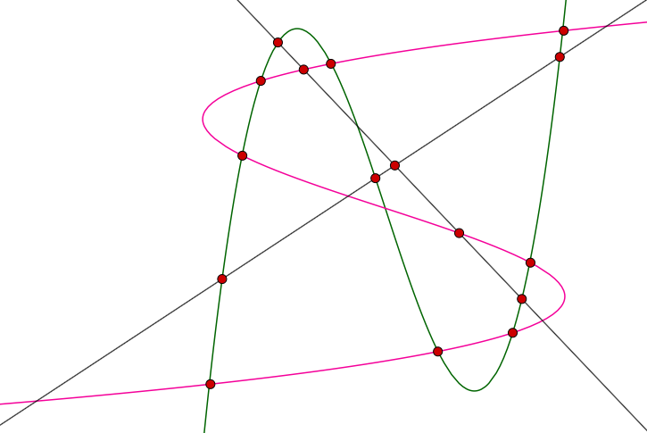 Figure 1
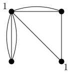 Figure 2
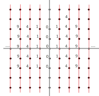 Figure 3
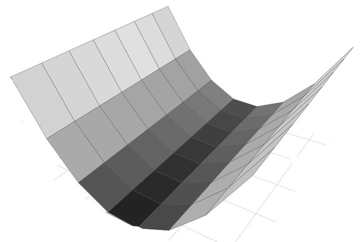 Figure 4
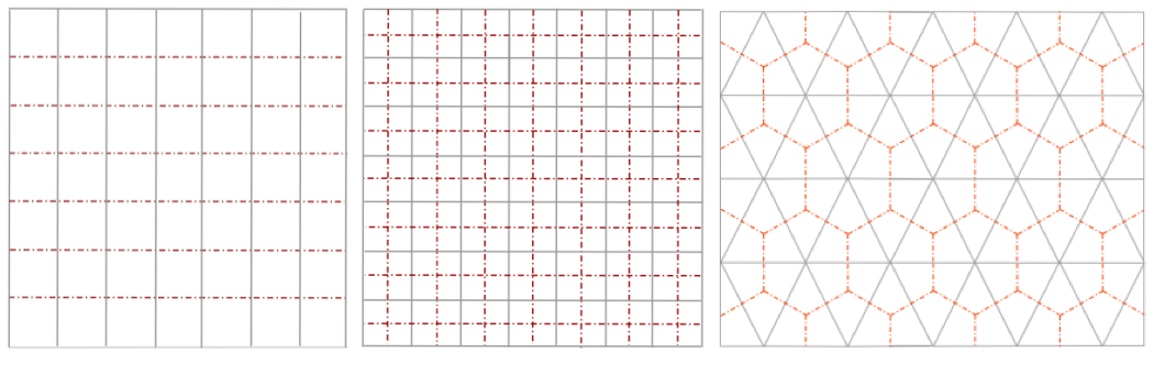 Figure 5
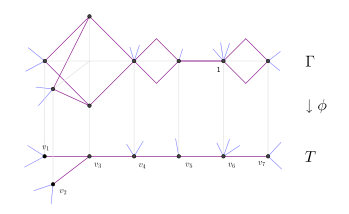 Figure 6
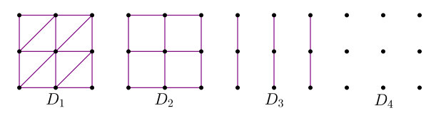 Figure 7
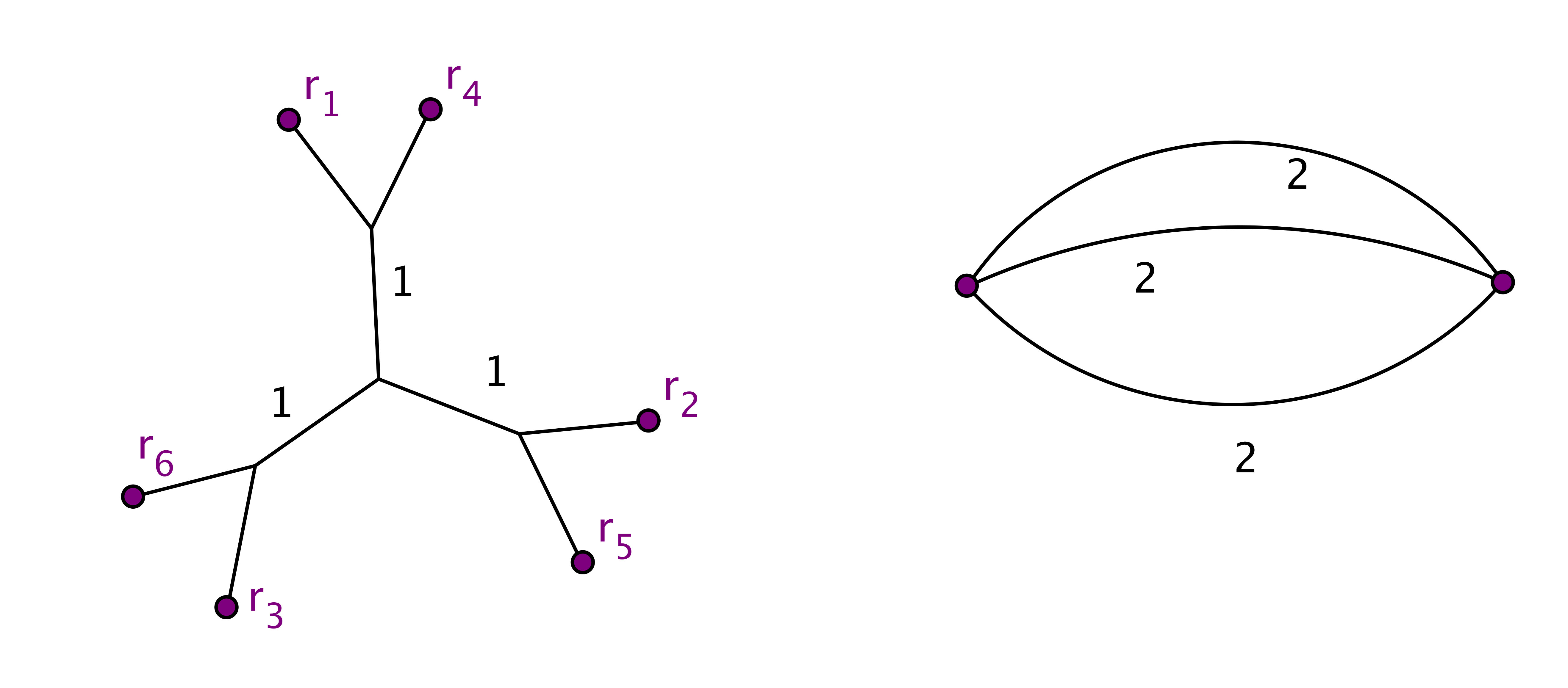 Figure 8
 Figure 9
 Figure 10
 Figure 11
 Figure 12
 Figure 13
 Figure 14
 Figure 15
 Figure 16
 Figure 17
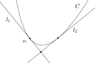 Figure 18
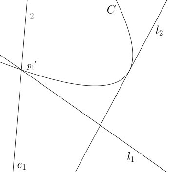 Figure 19
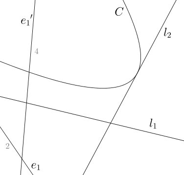 Figure 20
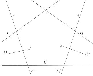 Figure 21
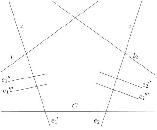 Figure 22
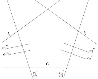 Figure 23
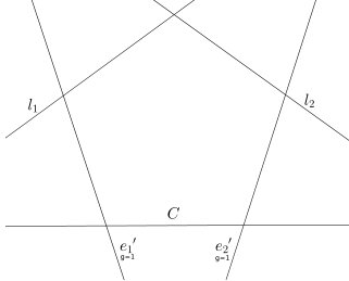 Figure 24
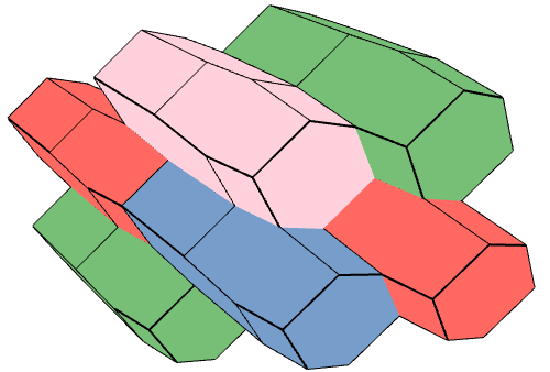 Figure 25
Peer Reviews
No public reviews on file for this paper yet. If you reviewed it on a platform where reviews are public (OpenReview, ICLR, NeurIPS, ICML), you can paste yours below so the community can read it here.
Videos
No videos yet. Explain this paper in a talk, walkthrough, or lecture? Add one.
Taxonomy
TopicsPolynomial and algebraic computation · Algebraic Geometry and Number Theory · Commutative Algebra and Its Applications
∎
11institutetext: Barbara Bolognese 22institutetext: The University of Sheffield, Sheffield, UK 22email: [email protected] 33institutetext: Madeline Brandt 44institutetext: Department of Mathematics, University of California, Berkeley, 970 Evans Hall, Berkeley, CA, 94720, 44email: [email protected] 55institutetext: Lynn Chua 66institutetext: Department of Electrical Engineering and Computer Science, University of California, Berkeley, 643 Soda Hall, Berkeley, CA, 94720, 66email: [email protected]
From Curves to Tropical Jacobians and Back
Barbara Bolognese
Madeline Brandt
Lynn Chua
Abstract
Given a curve defined over an algebraically closed field which is complete with respect to a nontrivial valuation, we study its tropical Jacobian. This is done by first tropicalizing the curve, and then computing the Jacobian of the resulting weighted metric graph. In general, it is not known how to find the abstract tropicalization of a curve defined by polynomial equations, since an embedded tropicalization may not be faithful, and there is no known algorithm for carrying out semistable reduction in practice. We solve this problem in the case of hyperelliptic curves by studying admissible covers. We also describe how to take a weighted metric graph and compute its period matrix, which gives its tropical Jacobian and tropical theta divisor. Lastly, we describe the present status of reversing this process, namely how to compute a curve which has a given matrix as its period matrix.
1 Introduction
We describe the process of taking a curve and finding its tropical Jacobian. We aim to carry out each step as algorithmically as possible, however, some steps cannot yet be completed in such a way. We now give a brief overview of the steps involved, which we depict in Figure 1.
Let be an algebraically closed field which is complete with respect to a non-archimedean valuation , and let be a nonsingular curve of genus over . Let be the valuation ring of with maximal ideal , and let be its residue field. We can associate to its abstract tropicalization, which is the dual weighted metric graph of the special fiber of a semistable model of . In practice, finding the abstract tropicalization of a general curve is difficult and there is no known algorithm to do this in general (CJar, , Remark 3). In this paper, we solve this problem for hyperelliptic curves, which is new to the literature, and discuss known results towards finding abstract tropicalizations of all curves.
Given , we compute its period matrix . This corresponds to the tropical Jacobian of the curve . By taking the Voronoi decomposition dual to the Delaunay subdivision corresponding to , we obtain the tropical theta divisor. This process can also be inverted. The set of period matrices that arise as the tropical Jacobian of a curve is the tropical Schottky locus. Starting with a principally polarized tropical abelian variety whose period matrix is known to lie in the tropical Schottky locus, we give a procedure to compute a curve whose tropical Jacobian corresponds to .
This process of associating a tropical Jacobian to a curve can also be carried out by looking at classical Jacobians of curves. Jacobians of curves are principally polarized abelian varieties in a natural way; they are the most well known and extensively studied among abelian varieties. Both algebraic curves and abelian varieties have extremely rich geometries, which cannot be fully understood in many cases. Jacobians provide a link between such geometries, and they often reveal hidden features of algebraic curves which cannot be uncovered otherwise. In order to associate a tropical Jacobian to a complex algebraic curve , one first constructs its classical Jacobian
[TABLE]
where we denote by the cotangent bundle of the curve. This complex torus admits a natural principal polarization , called the theta divisor, such that the pair is a principally polarized abelian variety. We can then obtain the tropical Jacobian by taking the Berkovich skeleton of the classical Jacobian. Baker-Rabinoff, and independently Viviani, proved that this alternative path gives the same result as the procedure we describe in this paper BR (15); Viv (13). However, the classical process hides more difficulties on the computational level and proves much more challenging to carry out in explicit examples. Methods have been implemented in the Maple package algcurves for computing Jacobians numerically over DP (11).
The structure of this paper is depicted in Figure 1. In Section 2 we find the abstract tropicalization of all hyperelliptic curves, a result which is new to this paper. Then, in Section 3 we discuss issues with embedded tropicalization, state some known results about certifying a faithful tropicalization, and outline the process of semistable reduction. This step of the procedure is far from being algorithmic, and this section focuses on examples which provide obstacles to doing this in general. In Section 4 we describe how to find the period matrix of a weighted metric graph. Then we define and give examples of the tropical Jacobian and its theta divisor in Section 5. In Section 6, we discuss the tropical Schottky problem. Finally, we describe the obstacles to reversing this process in Section 7.
2 Hyperelliptic Curves
We now study the problem of finding the abstract tropicalization of hyperelliptic curves. In the case of elliptic curves, the tropicalization can be completely described in terms of the -invariant KMM (08). Similarly, tropicalizations of genus 2 curves (all of which are hyperelliptic) can be described by studying tropical Igusa invariants Hel . This problem was also solved in genus 2 by studying the curve as a double cover of ramified at 6 points, as done in (RSS, 14, Section 5).
In this section, we generalize the latter method to find tropicalizations of all hyperelliptic curves, which was previously not known. Let be a nonsingular hyperelliptic curve of genus over , an algebraically closed field which is complete with respect to a nontrivial, non-archimedean valuation . Our goal is to find , the abstract tropicalization of .
We denote by the moduli space of genus curves with marked points, see HM (98) for a thorough introduction. The space maps surjectively onto the hyperelliptic locus inside by identifying each hyperelliptic curve of genus g with a double cover of ramified at marked points. When the characteristic of is not 2, the normal form for the equation of a hyperelliptic curve is where has degree , and the roots of are distinct. Then, these are precisely the ramification points.
The space is the tropicalization of . A phylogenetic tree is a metric tree with leaves labeled and no vertices of degree 2. Such a tree is uniquely specified by the distances between the leaves. We see that parametrizes the space of phylogenetic trees with leaves using the Plücker embedding to map into the Grassmannian (MS, 15, Chapter 4.3) :
[TABLE]
The distances are then given by for a suitable constant (RSS, 14, Section 5). Using the Neighbor Joining Algorithm (PS, 05, Algorithm 2.41), one can construct the unique tree, along with the lengths of its interior edges, using only the leaf distances as input. Since the lengths of leaf edges can only be defined up to adding a constant length to each leaf, we think of this tree as a metric graph where the leaves have infinite length and the interior edges have lengths as described.
This realizes as a dimensional fan inside (cf. (MS, 15, Section 2.5)). The space can be computed as a tropical subvariety of , since it has a tropical basis given by the Plücker relations for (MS, 15, Chapter 4.4). Each cone corresponds to a combinatorial type of tree (see Figure 2), and the dimension of each cone corresponds to the number of interior edges in the tree.
The next step in finding the tropicalization of the hyperelliptic curve is to take the corresponding point in , as a tree on leaves, and compute a weighted metric graph in . Figure 2 gives this correspondence in the case . We now give some definitions related to metric graphs in order to describe this correspondence for general , following Cha (13).
Definition 1
A metric graph is a metric space , together with a graph and a length function such that is obtained by gluing intervals of length , or by gluing rays to their endpoints, according to how they are connected in . In this case, the pair is called a model for . A *weighted metric graph * is a metric graph together with a weight function on its points , such that is finite.
We call edges of infinite length infinite leaves, and these only meet the rest of the graph in one endpoint. A bridge is an edge whose deletion increases the number of connected components.
The genus of a weighted metric graph (, ) is
[TABLE]
where is any model of . We say that two weighted metric graphs of genus are isomorphic if one can be obtained from the other via graph automorphisms, or by removing infinite leaves or leaf vertices with , together with the edge connected to it. In this way, every weighted metric graph has a minimal skeleton.
A model is loopless if there is no vertex with a loop edge. The canonical loopless model of , with genus of , is the graph with vertices
[TABLE]
If and are loopless models for metric graphs and , then a morphism of loopless models is a map of sets such that
- •
All vertices of map to vertices of .
- •
If maps to , then the endpoints of must also map to .
- •
If maps to , then the endpoints of must map to vertices of .
- •
Infinite leaves in map to infinite leaves in .
- •
If , then is an integer. These integers must be specified if the edges are infinite leaves.
We call an edge vertical if maps to a vertex of . We say that is harmonic if for every , the local degree
[TABLE]
is the same for all choices of . If it is positive, then is nondegenerate. The degree of a harmonic morphism is defined as
[TABLE]
We also say that satisfies the local Riemann-Hurwitz condition if:
[TABLE]
If satisfies this condition at every vertex in the canonical loopless model of , then is called an admissible cover CMR (16).
Definition 2
(Cha, 13, Theorem 1.3) Let be a weighted metric graph, and let denote its canonical loopless model. We say that is hyperelliptic if there exists a nondegenerate harmonic morphism of degree 2 from to a tree.
A hyperelliptic curve will always tropicalize to a hyperelliptic weighted metric graph, however not every hyperelliptic weighted metric graph is the tropicalization of a hyperelliptic curve.
Theorem 2.1
(ABBR, 15, Corollary 4.15)* Let be a minimal weighted metric graph of genus . Then there is a smooth proper hyperelliptic curve over of genus having as its minimal skeleton if and only if is hyperelliptic and for every the number of bridge edges adjacent to is at most .*
Lemma 1 and its proof give an algorithm for taking a tree with infinite leaves and obtaining a metric graph which is an admissible cover of the tree.
Lemma 1
Every tree with infinite leaves has an admissible cover by a unique hyperelliptic metric graph of genus , and is harmonic of degree 2.
Proof
Let be a tree with infinite leaves. If all infinite leaves are deleted, then a finite tree remains. Let be the vertices of , ordered such that the distance from to is greater than or equal to the distance from to , for .
We construct iteratively by building the preimage of each vertex , asserting along the way that the local Riemann-Hurwitz condition holds. This also gives an algorithm for finding . We begin with , which has a positive number of leaf edges in . Since has degree 2, it must be locally of degree 1 or 2 at every vertex of . Since the preimage of each infinite leaf must be an infinite leaf, we will attach infinite leaves at the preimage in .
At any vertex in with infinite leaves, has local degree , hence we will attach to an infinite leaf such that . Then, there is a unique vertex in the preimage . Otherwise, there would need to be another edge in the preimage of each leaf, so the degree of the morphism would be greater than 2.
Let be the edge connecting to some other . There are two possibilities:
The preimage of is two edges in , each with length . The local Riemann-Hurwitz equation reads
[TABLE]
This is only possible if is even, and has weight . 2. 2.
The preimage of is one edge in , with length . The local Riemann-Hurwitz equation reads
[TABLE]
This is only possible if is odd, and has weight .
Now, we proceed to the other vertices. As long as the order of the vertices is respected, at each vertex there will be at most one edge whose preimage in we do not know. Then, what happens at can be completely determined by studying the local Riemann-Hurwitz data. For , let be the number of infinite leaves at plus the number of edges such that , , and is a bridge in . If , then either 1 or 2 holds. However, it is possible that , in which case we have a third possibility:
If , let . The local Riemann-Hurwitz equation reads:
[TABLE]
Then we must have and , which implies that there are two vertices in .
Finally, we glue the pieces of as specified by , and contract the leaf edges on . The fact that has genus is a consequence of the local Riemann-Hurwitz condition. ∎
We remark that this process did not require the fact that the tree had an odd number of leaves. Indeed, if one repeats this procedure for such a tree, a hyperelliptic metric graph will be obtained. However, this graph is not the tropicalization of a hyperelliptic curve.
Example 1
In Figure 3, we have a tree with vertices labelled . Beginning with , we observe that , which means that the edge from to has two edges in its preimage. The same is true for . Moving on to , we see that , which means that has two points in which map to it. We can connect the edges from and to the two points in . Since has two points, the edge from to corresponds to two edges in , so , which means that the edge from to also splits. Next, , which means that the edge from to corresponds to a bridge in . Then, , which means that the edge to splits, and the vertex mapping to has genus . Lastly, since , the point mapping to has genus 0. All edges depicted in the image have the same length as the corresponding edges in the tree, except for the bridge, which has length equal to half the length of the corresponding edge in the tree.
The following theorem shows that this metric graph is actually the tropicalization of a hyperelliptic curve.
Theorem 2.2
Let be an integer. Let be a hyperelliptic curve of genus over , given by taking the double cover of ramified at points . If is the tree which corresponds to the tropicalization of with the marked points described above, and is the unique hyperelliptic weighted metric graph which admits an admissible cover to , then is the abstract tropicalization of .
Proof
This follows from CMR (16), Remark 20 and Theorem 4. Indeed, the hyperelliptic locus of can be understood as the space of admissible covers with ramification points of order 2. Its tropicalization is constructed and studied in CMR (16). The space is the Berkovich analytification of , and thus a point is represented by an admissible cover over with ramification points of order 2. By Theorem 4 in CMR (16), the diagram
[TABLE]
commutes. The morphisms take a cover to its source curve, marked at the entire inverse image of the branch locus, and the morphisms take a cover to its base curve, marked at its branch points. We start with an element of , and we wish to find . The unicity in Lemma 1 enables us to find an inverse for . Then , and so by commutativity of the diagram, . ∎
Example 2
((Stuar, , Problem 2 on Curves)) Consider the curve
[TABLE]
with the 5-adic valuation. In , this gives us the point
[TABLE]
When is any integer, this gives us a tree metric of
[TABLE]
Then, this is a metric for the tree on the left of Figure 4, and the metric graph on the right.
3 Other Curves
Outside of the hyperelliptic case, finding the abstract tropicalization of a curve is very hard. In this section, we highlight some of the difficulties and discuss two approaches to this problem: faithful tropicalization and semistable reduction. We offer the following example as motivation for why this is a difficult problem.
Example 3
((Stuar, , Problem 9 on Abelian Combinatorics)) We begin with a curve in , given by the zero locus of
[TABLE]
defined over . Here, the induced regular subdivision of the Newton polygon will be trivial, since the 2-adic valuation of the coefficients on the terms is each 0. Therefore, we can detect no information about the structure of the abstract tropicalization from this embedded tropicalization. In Example 4, we will pick a nice enough change of coordinates to allow us to find a faithful tropicalization.
3.1 Faithful Tropicalization
We briefly discuss the Berkovich skeleton of a curve. Let be an algebraically closed field which is complete with respect to a nontrivial, nonarchimedean valuation . Let be a nonsingular curve defined over . To simplify the definitions in this exposition, we restrict to the case when is affine, and for a thorough explanation the reader may consult Ber (93). The Berkovich analytification is a topological space whose ground set consists of all multiplicative seminorms on the coordinate ring that are compatible with the valuation on . It has the coarsest topology such that for every , the map sending a seminorm to is continuous. We note that this is different from the metric structure, see (BPR, 13, 5.3). When is a smooth, proper, geometrically integral curve of genus greater than or equal to 1, admits strong deformation retracts onto finite metric graphs called skeletons of Bak (08). There is also a unique minimal skeleton.
The minimal skeleton of the Berkovich analytification is the same metric graph as the dual graph of the special fiber of a stable model of a curve . Let be an embedding of , which gives generators of the coordinate ring . Denote its embedded tropicalization by . Details about how to carry this out (including how to find the metric on ) can be found in MS (15). We can relate the Berkovich analytification to embedded tropicalizations in the following way.
Theorem 3.1
(Pay, 09, Theorem 1.1)* Let be an affine variety over . Then there is a homeomorphism*
[TABLE]
The homeomorphism is given by the inverse limit of maps defined by
[TABLE]
where denotes the norm corresponding to the point . The image of this map is equal to .
Given just one embedded tropicalization, we want to detect information about the Berkovich skeleton. This is the problem of certifying faithfulness, as studied in (BPR, 16, 5.23).
In some cases, the embedded tropicalization contains enough information to determine the structure of the skeleton of .
Theorem 3.2
Let be a smooth curve in of genus . Further, suppose that , all vertices of are trivalent, and all edges have multiplicity 1. Then the minimal skeleta of and are isometric. In particular, if is a smooth curve in whose Newton polygon and subdivision form a unimodular triangulation, then the minimal skeleta of and are isometric.
Proof
This follows from a result of Baker, Payne, and Rabinoff (BPR, 16, Corollary 5.2.8) who assume instead that all vertices of are trivalent, all edges have multiplicity 1, has no leaves, and that . In our case, we are trying to detect information about the minimal skeleton of , so we have reduced to the case in which we can remove assumptions about from the hypotheses.
In particular, we have that , so in the case when , we also have . Furthermore, it is only possible that has leaves when . ∎
The next example illustrates how to apply this Theorem to find the metric graph of the curve given in Problem 9.
Example 4 (Problem 9, Continued)
We apply a change of coordinates
[TABLE]
to obtain
[TABLE]
We calculate the regular subdivision of the Newton polyton in Polymake 3.0 GJ (00), weighted by the 2-adic valuations of the coefficients.
The embedded tropicalization and corresponding metric graph, with edge lengths, are depicted in Figure 5. Since we have that all vertices are trivalent, all edges have multiplicity 1, and , we have by Theorem 3.2 that this is the abstract tropicalization of the curve.
Example 5
We offer another example to illustrate some of the shortcomings of Theorem 3.2. We will ultimately need to use semistable reduction to solve the problem in this case.
Consider the curve in over defined by
[TABLE]
Tropicalizing with this embedding, we obtain the embedded tropicalization in Figure 6.
Since this is not a unimodular triangulation, Theorem 3.2 does not allow us to draw any conclusions. However, we will see in the next section that this is, in fact, a faithful tropicalization.
3.2 Semistable Reduction
If we cannot certify faithfulness of a tropicalization (as in Example 5), we can instead find the metric graph by taking the dual graph of a semistable model for BPR (13). To this end, we outline the process of finding the semistable model of a curve .
Let be a reduced, nodal curve over , and for each irreducible component of , let be the normalization of . We say that is semistable if every smooth rational component meets the rest of the curve in at least two points, or every component of has at least 2 points such that is a singularity in .
Let be the valuation ring of . Then contains two points: one corresponding to the zero ideal and another corresponding to , the maximal ideal of . If is a scheme over , we call the fiber of the the point corresponding to the generic fiber, and the fiber over the point corresponding to the special fiber.
Definition 3
If is any finite type scheme over , a model for is a flat and finite type scheme over whose generic fiber is isomorphic to . We call this model semistable if the special fiber is a semistable curve over .
The curve always admits a semistable model, by the Semistable Reduction Theorem. The proofs of this theorem contain somewhat algorithmic approaches, see DM (69) and AW (12).
Now, we describe a procedure for finding a semistable model for the curve when has characteristic 0. A good reference is HM (98). The first step is to blow up the total space , removing any singularities in the special fiber, to arrive at a family whose special fiber is a nodal curve. At this point, our work is not yet done because the resulting curve will be nonreduced.
Example 6
(Example 5, Continued) In this case, the special fiber is a conic with two tangent lines, depicted in Figure 7(a). We denote the conic by and the two lines by and . We begin by blowing up the total space at the point . The result, depicted in Figure 7(b), is that and are no longer tangent, but they do intersect in the exceptional divisor, which we call . The exceptional divisor has multiplicity 2, coming from the multiplicity of the point . In the figures, we denote the multiplicities of the components with grey integers, and a component with no integer is assumed to have multiplicity 1.
Next, we blow up the total space at the point labelled to get Figure 8(c). We denote the new exceptional divisor by with multiplicity 4, and the curves and no longer intersect. All points except are either smooth or have nodal singularities, so we repeat these two blowups here, obtaining the configuration in Figure 8(d).
Remark 1
At this point, we have a family whose special fiber only has nodes as singularities, but it is not reduced. To fix this, we make successive base changes of prime order . Explicitly, we take the -th cover of the family branched along the special fiber. Then, if is a component of multiplicity in the special fiber, either does not divide , in which case is in the branch locus, or else we obtain copies of branched along the points where meets the branch locus, and the multiplicity is reduced by .
Example 7
(Example 5, Continued) We must make two base changes of order 2. Starting with Figure 8(d) above, we see that , , and are in the branch locus. The curves and are replaced by the double cover of each of them branched at 2 points, which is again a rational curve. We continue to call these and , and they each have multiplicity 2. Then, and are disjoint from the branch locus, so each one is replaced by two disjoint rational curves. The result is depicted in Figure 9(e). In the second base change of order 2, all components except and are in the branch locus. The curves and each meet the branch locus in 4 points, which, by the Riemann-Hurwitz theorem, means they will be replaced by genus 1 curves. The result is depicted in Figure 9(f).
The last step is to blow down all rational curves which meet the rest of the fiber exactly once, depicted in Figure 10. This gives us a semistable model of .
3.3 Weighted Metric Graphs
From a faithful tropicalization, the abstract tropicalization of a curve can be obtained simply by taking the minimal skeleton of . Given a semistable model of , this coincides with the dual graph of BPR (13).
Definition 4
Let be the irreducible components of , the special fiber of a semistable model of . The dual graph of , , is defined with vertices corresponding to the components , where we set . There is an edge between and if the corresponding components and intersect in a node . Then, the completion of the local ring is isomorphic to , where is the valuation ring of , and , the maximal ideal of . Then, we define .
Example 8
(Example 5, Continued)
Taking the dual graph of the semistable model found in the previous example, we obtain a cycle with two vertices of weight 1. By (BPR, 16, Theorem 5.24), the cycle that we observed in the embedded tropicalization actually gave a faithful tropicalization. This implies that the metric graph is as depicted in Figure 11.
4 Period Matrices of Weighted Metric Graphs
Recall that a weighted metric graph is a metric graph with a model , a function on assigning nonnegative weights to the vertices, and a function on assigning positive lengths to the edges. Given , we describe a procedure to compute its period matrix, following MZ (08); BMV (11); Cha (12).
Fix an orientation of the edges of . For any , denote the source vertex by and the target vertex by . Let be or . The spaces of 0-chains and 1-chains of with coefficients in are defined as
[TABLE]
The module is equipped with the inner product
[TABLE]
The boundary map acts linearly on 1-chains by mapping an edge to . The kernel of this map is the first homology group of , whose rank is
[TABLE]
Let , and let be the genus of , defined as . Consider the positive semidefinite form on , which vanishes on the second summand and is defined on by
[TABLE]
Definition 5
Let be a basis of . Then, we obtain an identification of the lattice with . Hence, we may express as a positive semidefinite matrix, called the period matrix of . Choosing a different basis gives another matrix related by an action of .
To find the period matrix, first fix an arbitrary orientation of the edges of . We then pick a spanning tree of . Label the edges such that are not in , and are in , where . Then , for , contains a unique cycle of . The cycles form a cycle basis of .
We traverse each cycle according to the direction specified by . We compute a row vector of length , representing the direction of edges of in this traversal. For each edge in , let the -th entry of be if is in the correct orientation in the cycle, if it is in the wrong orientation, and 0 if it is not in the cycle. Let be the matrix whose -th row is . The matrix has an interpretation in matroid theory as a totally unimodular matrix representing the cographic matroid of Oxl (11).
Suppose that all vertices have weight zero, such that . Let be the diagonal matrix with entries . Then the period matrix is given by . If we label the columns of by , the period matrix equals
[TABLE]
Thus the cone of all matrices that are period matrices of , allowing the edge lengths to vary, is the rational open polyhedral cone
[TABLE]
If has vertices of nonzero weight, the period matrix is given by the construction above with additional rows and columns with zero entries.
Example 9
Consider the complete graph on 4 vertices in Figure 12.
We indicate in the figure an arbitrary choice of the edge orientations, and we choose the spanning tree consisting of the edges . This corresponds to the cycle basis , , and . Next, we compute the matrix as
[TABLE]
Let be the diagonal matrix with entries along the diagonal. The period matrix is then
[TABLE]
In the next section, we will use period matrices to define and study tropical Jacobians of curves as principally polarized tropical abelian varieties.
5 Tropical Jacobians
Let be the set of symmetric positive semidefinite matrices with rational nullspace, meaning that their kernels have bases defined over . The group acts on by for all , .
We define a tropical torus of dimension as a quotient , where is a lattice of rank in . A polarization on is given by a quadratic form on . Following BMV (11); Cha (12), we call the pair a principally polarized tropical abelian variety (pptav), when .
Two pptavs are isomorphic if there is some that maps one lattice to the other, and acts on one quadratic form to give the other. We can choose a representative of each isomorphism class in the form , where is an element of the quotient of by the action of . The points of this space are in bijection with the points of the moduli space of principally polarized tropical abelian varieties, which we denote by . We will describe the structure of in Section 6.
Definition 6
The tropical Jacobian of a curve is , where is the period matrix of the curve.
The tropical Jacobian is our primary example of a principally polarized tropical abelian variety. The period matrix induces a Delaunay subdivision of , which has an associated Voronoi decomposition giving the tropical theta divisior of the tropical Jacobian. We describe this in more detail below.
Given , consider the map
[TABLE]
Take the convex hull of image of in . By projecting down the lower faces via the morphism which forgets the last coordinate, we obtain a periodic dicing of the lattice , called the Delaunay subdivision of . This operation corresponds, naively speaking, to looking at the polyhedron from below and recording on the lattice only the faces that we see. This is an infinite and periodic analogue of taking the regular subdivision of a polytope induced by weights on the vertices.
Remark 2
There is in the literature much discordance about the spelling of the name Delaunay. The source of such discordance lies in the fact that Boris Nicolaevich Delaunay was a Russian mathematician, hence the correct transliteration of his last name from Cyrillic is much debated (since he himself used the two versions “Delaunay” and “Delone” when he signed his papers). One must notice, however, that the name itself is of French origin: indeed, Boris Delaunay got his last name from the French Army officer De Launay, who was captured in Russia during Napoleon’s invasion of 1812 and, after marrying a Russian noblewoman, settled down in Russia (see Roz ). Hence we decided to use the French transliteration, it being closer to the original name.
Example 10
Consider the matrix . The function is given by . If we now take the convex hull of the points in the image of , we obtain the following picture on the left, together with the Delaunay subdivision on the right.
Given a Delaunay decomposition, one can consider the dual decomposition, called the Voronoi decomposition. This is illustrated in Figure 14 for .
The Voronoi decomposition corresponds to the tropical theta divisor associated to a pptav , which is the tropical hypersurface in defined by the theta function
[TABLE]
It is possible to give a more manageable description of the tropical theta divisor in virtue of Theorem 5.1, as we are about to explain. Let be a weighted metric graph , and let be a fixed basepoint. Let be a basis of . For any point in , let describe any path from to . Then, take the inner product (defined in Equation 15) of with each element of the cycle basis to obtain a point of , given by
[TABLE]
This does not depend on the choice of path from to . By the identification with induced by the choice of cycle basis, this defines a point of the tropical Jacobian. We may extend this map linearly so that it is defined on all divisors on . By a divisor on , we mean a finite formal integer linear combination of points in . Then the map is called the tropical Abel-Jacobi map MZ (08).
Given a divisor , where and , define the degree of as . We say that is effective if for all . Let be the image of degree effective divisors under the tropical Abel-Jacobi map.
Theorem 5.1 (Corollary 8.6, MZ (08))
The set is the tropical theta divisor up to translation.
Example 11 (Example 9, Continued)
Delaunay subdivisions also arise in many other branches of mathematics, for example in lattice packing or covering problems. In this context, Sikirić wrote a GAP GAP (16) software package polyhedral DS (13). Using this package, we compute that the Delaunay subdivision of the quadratic form in Equation 21 is given by six tetrahedra in the unit cube, all of which share the great diagonal as an edge. We also compute using polyhedral the Voronoi decomposition dual to this Delaunay subdivision, which gives a tiling of by permutohedra as illustrated in Figure 15. This is the tropical theta divisor, with -vector . In Figure 16, we illustrate the correspondence described by Theorem 5.1 between and the tropical theta divisor.
6 Tropical Schottky Problem
We describe the structure of the moduli space in this section, using Voronoi reduction theory. Given a Delaunay subdivision , define the set of matrices that have as their Delaunay subdivision to be
[TABLE]
The secondary cone of is the Euclidean closure of in , and is a closed rational polyhedral cone. There is an action of on the set of secondary cones, induced by its action on .
Theorem 6.1 (Vor (08))
The set of secondary cones forms an infinite polyhedral fan whose support is , known as the second Voronoi decomposition. There are only finitely many -orbits of this set of secondary cones.
By this theorem, we can choose Delaunay subdivisions of , such that the corresponding secondary cones are representatives for -equivalence classes of secondary cones. The moduli space is a stacky fan whose cells correspond to these classes Cha (12); BMV (11). More precisely, for each Delaunay subdivision , consider the stabilizer
[TABLE]
Define the cell
[TABLE]
as the quotient of the secondary cone by the stabilizer. Then we have
[TABLE]
where we take the disjoint union of the cells and quotient by the equivalence relation induced by -equivalence of matrices in , which corresponds to gluing the cones.
Example 12
In genus two, we can choose the Delaunay subdivisions as shown in Figure 17. These have the property that their secondary cones give representatives for -equivalence classes of secondary cones.
The corresponding secondary cones are as follows.
[TABLE]
The tropical Torelli map sends a weighted metric graph of genus to its tropical Jacobian, which is the element of corresponding to its period matrix. The image of this map is called the tropical Schottky locus, which has a characterization using matroid theory.
Given a graph , we can define a cographic matroid (see Oxl (11) for an introduction to matroid theory). is representable by a totally unimodular matrix, constructed as the matrix in Section 4. The cone defined in Equation 19 is a secondary cone in . The -equivalence class of is independent of the choice of totally unimodular matrix representing . Hence we can associate to a unique cell of , corresponding to this equivalence class of secondary cones.
A matroid is simple if it has no loops and no parallel elements. We define the following stacky subfan of corresponding to simple cographic matroids,
[TABLE]
The image of the tropical Torelli map is BMV (11); Cha (12), and we call the tropical Schottky locus. When , , hence every element of is a period matrix of a weighted metric graph . But when , this inclusion is proper. For example, has 25 cells while has 61 cells, and has 92 cells while has 179433 cells, according to the computations in Cha (12).
From the classical perspective, the association , where is the Jacobian of defined in the introduction, gives the Torelli map
[TABLE]
Here denotes the moduli space of smooth genus curves, while denotes the moduli space of -dimensional abelian varieties with a principal polarization. The content of Torelli’s theorem is precisely the injectivity of the Torelli map, which in fact can be proved to be dominant for . Its image, i.e. the locus inside the moduli space of principally polarized abelian varieties, is called the Schottky locus and its complete description required several decades of work by many. The injectivity of the Torelli morphism implies, in particular, that we can always reconstruct an algebraic curve from its principally polarized Jacobian. The characterization of the Schottky locus was first worked out in genus 4 by Schottky himself and Jung (cf. SJ (09)) via theta characteristics. Many other approaches followed in history for higher genus: the work by Andreotti and Mayer (AM (67)), Matsusaka and Ran M*+* (59); Ran (80)) and Shiota (Shi (86)) are worth mentioning. For extensive surveys see e.g. Arb (99); Gru (12).
7 …and Back
The process we have described so far produces the tropical Jacobian of a curve given its defining equations. Now, we discuss whether it is possible to take a principally polarized tropical abelian variety X in the tropical Schottky locus, and produce a curve whose tropical Jacobian is precisely X. We remark that several of the steps described in the previous sections are far from being one-to-one. Indeed, many algebraic curves have the same abstract tropicalization; for example all curves with a smooth stable model tropicalize to a single weighted vertex. In the same fashion, the non-injectivity of the tropical Torelli map (see e.g. BMV (11); Cha (12)) implies that the same positive semidefinite matrix can be associated to more than one weighted metric graph. The purpose of this section is therefore to construct an arbitrary curve with a given tropical Jacobian.
7.1 From Tropical Jacobians to Positive Semidefinite Matrices
Let be a tropical Jacobian, and fix an isomorphism . The tropical theta divisor , as we remarked in Section 5, is a Voronoi decomposition dual to a Delaunay subdivision .
We can describe by a collection of hyperplanes , such that the lattice translates by of these hyperplanes cut out the polytopes in . Following (MV, 12, Fact 4.1.4) and ER (94), we can choose these hyperplanes with normal vectors such that the matrix with as its columns is simple unimodular. The secondary cone of is then
[TABLE]
Thus any quadratic form lying in the positive span of the rank one forms , for , will have Delaunay subdivision . In particular, we can take
[TABLE]
7.2 From Positive Semidefinite Matrices to Weighted Metric Graphs
Fix , and let be a matrix in . If is not positive definite, we can do a change of basis such that has a postive definite submatrix and remaining entries zero. This corresponds to adding weights on the vertices of the graph, which can be done arbitrarily as long as every weight zero vertex has degree at least 3. Hence without loss of generality we assume that is positive definite. Our goal is to first determine if corresponds to an element of the tropical Schottky locus, and if so, to find a weighted metric graph that has as its period matrix.
First consider all combinatorial types of simple graphs with genus less than or equal to . We compute their corresponding secondary cones, as defined in Equation 19. Let be the set of these secondary cones. We compute the secondary cone of , as defined in Equation 25, which can be done using polyhedral DS (13). The underlying theory is described in Sch (09). We then check if is -equivalent to any cone in . This can be done using polyhedral DS (13) with external calls to the program ISOM by Plesken and Souvignier PS (95, 97), see (DSGSW, 16, Section 4) for the implementation details.
If is not equivalent to any cone in , then is not the period matrix of a weighted metric graph . Otherwise, let be a cone in that is in the same -equivalence class as , and let be the graph from which we computed . Let such that maps to , then maps to a matrix in .
From Equation 19, we can write , and so for some . Then is the period matrix of with edge lengths , by Equation 18. Since the transformation corresponds to a different choice of cycle basis, we have constructed a metric graph with as its period matrix.
Example 13
Consider the positive definite matrix
[TABLE]
Using polyhedral, we compute that is -equivalent to the cone corresponding to the weighted metric graph in Figure 18, via the transformation
[TABLE]
Hence is in the tropical Schottky locus, and is the period matrix of the metric graph in Figure 18, with the cycle basis consisting of the cycles , , , and . We compute the edge lengths by expressing as a linear combination of the extreme rays of .
As of the time of writing, this algorithm is impractical for genus greater than 5, as the classification of Delaunay subdivisions is known only up to dimension 5 DSGSW (16). For more details about the genus 4 case, refer to future work with M. Kummer and B. Sturmfels.
7.3 From Weighted Metric Graphs to Algebraic Curves
Lastly, we wish to take a weighted metric graph and produce equations defining a curve which tropicalizes to . Any weighted metric graph arises through tropicalization (ACP, 15, Theorem 1.2.1). Given a smooth curve with as its tropicalization, there exists a rational map such that the restriction of to the skeleton is an isometry onto its image (BR, 15, Theorem 8.2). Since is not required to be a closed immersion, however, this does not necessarily give a faithful tropicalization, see (BR, 15, Remark 8.5).
The paper CFPU (15) also studies this question for a specific class of metric graphs. They give a method for producing curves over , embedded in a toric scheme and with a faithful tropicalization to the input metric graph . They start by defining a suitable nodal curve whose dual graph is a model for , and use deformation theory to show that the nodal curve can be lifted to a proper, flat, semistable curve over with the nodal curve as its special fiber, which tropicalizes to .
We now describe a procedure for finding a nodal curve over whose dual graph is a model for . Let be a weighted stable graph of genus with infinite edges. Recall that a stable graph is a connected graph such that each vertex of weight zero has valence at least three. The dual graph of a stable curve is always a stable graph.
The original idea for this procedure is due to Kollár, cf. Kol (14), and works in a much more general setup. Suppose that the stable graph is such that:
For each vertex , the weight is of the form
[TABLE]
for some integer . 2. 2.
For each two vertices , one has
[TABLE]
where denotes the number of edges between and .
Then every component of is realizable by a curve in , and it is possible to achieve the right number of intersection points between every two components. More precisely, one can proceed as follows:
Label the vertices as . For each , take a general smooth plane curve of degree . 2. 2.
We have now a reducible plane curve , whose irreducible components are the curves of degree (and hence, by the genus degree formula, of genus ). Any two components and will intersect in points, by Bézout’s formula. We choose any of those, and set . 3. 3.
Take the blow up of at all the points chosen for each and , which we will label by :
[TABLE]
and consider the proper transform of in . 4. 4.
Now, lives in the product . Embed in via a Segre embedding, and take the image of . This will now be a projective curve with components of the correct genera (as the genus is a birational invariant), and any two components will intersect precisely at the correct number of points. Hence its dual graph will be .
Example 14
Consider the graph in Figure 19.
It has two components of genus zero and two components of genus one, which we can realize as a pair of lines (respectively, of cubics) in general position in . The two lines will intersect in a point, the two cubics in nine points and each cubic will intersect each line in three points. The corresponding curve arrangement is as shown in Figure 20.
We need to blow up eight of the nine intersection points between the two cubics, since they correspond to edges between the components of genus one in the graph. Moreover, the two components of genus zero do not share an edge, hence the unique intersection point between the two lines must be blown up, as well as the three intersection points of a chosen cubic with a line, two out of the three intersection point with the remaining line, and one of the three intersection points of the first cubic with the second line. In Figure 20, these point are marked in red. The result will be a curve in , whose components will have the correct genera and will intersect at the correct number of points, and whose equations can be explicitly computed.
Remark 3
The theory shows that it is, in principle, possible to find a smooth curve over with a prescribed metric graph as its tropicalization. For certain types of graphs, more work has been done in this direction CFPU (15). However, this problem is far from being solved in full generality in an algorithmic way, and this could be the subject of future research.
Acknowledgements.
This article was initiated during the Apprenticeship Weeks (22 August-2 September 2016), led by Bernd Sturmfels, as part of the Combinatorial Algebraic Geometry Semester at the Fields Institute. We heartily thank Bernd Sturmfels for leading the Apprenticeship Weeks and for providing many valuable insights, ideas and comments. We would also like to thank Melody Chan, for providing several useful directions which were encoded in the paper and for suggesting Example 5. We are grateful to Renzo Cavalieri, for a long, illuminating conversation about admissible covers, and Sam Payne and Martin Ulirsch for suggesting references and for clarifying some obscure points. We also thank Achill Schürmann and Mathieu Dutour Sikirić for their input on software for working with Delaunay subdivisions. The first author was supported by the Fields Institute for Research in Mathematical Sciences. The second author was supported by the National Science Foundation Graduate Research Fellowship under Grant No. DGE 1106400 and the Max Planck Institute for Mathematics in the Sciences, Leipzig. The third author was supported by a UC Berkeley University Fellowship and the Max Planck Institute for Mathematics in the Sciences, Leipzig.
The reference list from the paper itself. Each links out to its DOI / PubMed record.
- 1ABBR (15) Omid Amini, Matthew Baker, Erwan Brugallé, and Joseph Rabinoff, Lifting harmonic morphisms II: Tropical curves and metrized complexes , Algebra & Number Theory 9 (2015), no. 2, 267–315.
- 2ACP (15) Dan Abramovich, Lucia Caporaso, and Sam Payne, The tropicalization of the moduli space of curves , Ann. Sci. Ec. Norm. Sup 48 (2015), no. 4, 765–809.
- 3AM (67) Aldo Andreotti and AL Mayer, On period relations for abelian integrals on algebraic curves , Annali della Scuola Normale Superiore di Pisa-Classe di Scienze 21 (1967), no. 2, 189–238.
- 4Arb (99) Enrico Arbarello, Survey of work on the schottky problem up to 1996 , Red Book of Varieties and Schemes, 2nd Edition 1358 (1999), 287–291.
- 5AW (12) Kai Arzdorf and Stefan Wewers, Another proof of the semistable reduction theorem , ar Xiv:1211.4624 (2012).
- 6Bak (08) Matthew Baker, An introduction to Berkovich analytic spaces and non-Archimedean potential theory on curves , p 𝑝 p -adic geometry, Univ. Lecture Ser., vol. 45, Amer. Math. Soc., Providence, RI, 2008, pp. 123–174.
- 7Ber (93) Vladimir G. Berkovich, Étale cohomology for non-Archimedean analytic spaces , Institut des Hautes Études Scientifiques. Publications Mathématiques (1993), no. 78, 5–161.
- 8BMV (11) Silvia Brannetti, Margarida Melo, and Filippo Viviani, On the tropical Torelli map , Advances in Mathematics 226 (2011), no. 3, 2546–2586.