K\"ahler structures on spaces of framed curves
Tom Needham

TL;DR
This paper characterizes the space of framed loops in three-dimensional space as an infinite-dimensional K"ahler manifold, describes its geometric properties, and relates it to polygon spaces and planar loops, with implications for shape analysis.
Contribution
It identifies the framed loop space with a complex Grassmannian, explicitly describes geodesics, and analyzes curvature and symmetries, extending previous work on polygon and planar loop spaces.
Findings
Framed loop space is an infinite-dimensional K"ahler manifold.
The space of immersed loops is a symplectic reduction of the framed loop space.
The space and its quotient are nonnegatively curved.
Abstract
We consider the space of Euclidean similarity classes of framed loops in . Framed loop space is shown to be an infinite-dimensional K\"{a}hler manifold by identifying it with a complex Grassmannian. We show that the space of isometrically immersed loops studied by Millson and Zombro is realized as the symplectic reduction of by the action of the based loop group of the circle, giving a smooth version of a result of Hausmann and Knutson on polygon space. The identification with a Grassmannian allows us to describe the geodesics of explicitly. Using this description, we show that and its quotient by the reparameterization group are nonnegatively curved. We also show that the planar loop space studied by Younes, Michor, Shah and Mumford in the context of computer vision embeds in as a totally geodesic,…
Click any figure to enlarge with its caption.
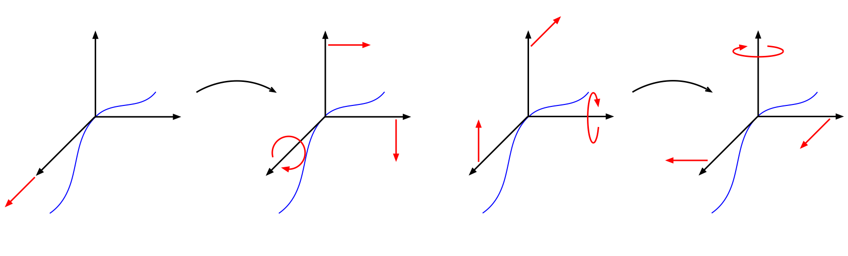 Figure 7
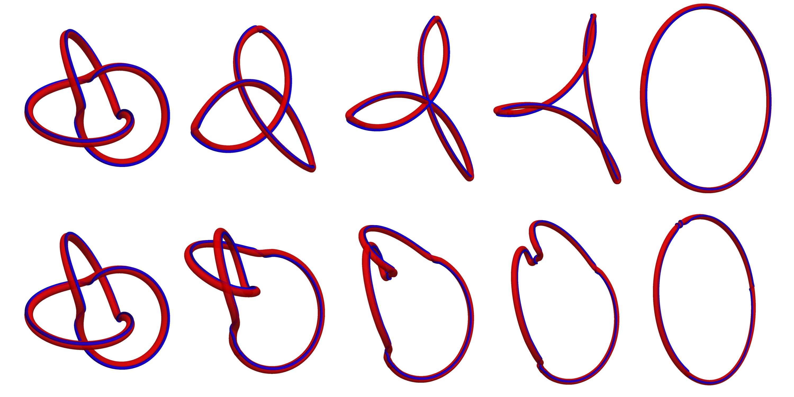 Figure 2
Peer Reviews
No public reviews on file for this paper yet. If you reviewed it on a platform where reviews are public (OpenReview, ICLR, NeurIPS, ICML), you can paste yours below so the community can read it here.
Videos
No videos yet. Explain this paper in a talk, walkthrough, or lecture? Add one.
Taxonomy
TopicsMorphological variations and asymmetry
Kähler structures on spaces of framed curves
Tom Needham
Department of Mathematics, The Ohio State University
Abstract.
We consider the space of Euclidean similarity classes of framed loops in . Framed loop space is shown to be an infinite-dimensional Kähler manifold by identifying it with a complex Grassmannian. We show that the space of isometrically immersed loops studied by Millson and Zombro is realized as the symplectic reduction of by the action of the based loop group of the circle, giving a smooth version of a result of Hausmann and Knutson on polygon space. The identification with a Grassmannian allows us to describe the geodesics of explicitly. Using this description, we show that and its quotient by the reparameterization group are nonnegatively curved. We also show that the planar loop space studied by Younes, Michor, Shah and Mumford in the context of computer vision embeds in as a totally geodesic, Lagrangian submanifold. The action of the reparameterization group on is shown to be Hamiltonian and this is used to characterize the critical points of the weighted total twist functional.
1. Introduction
Let denote the space of -edge polygons in with fixed edgelengths given by , where two polygons are identified if they differ by a rigid motion. In [15], Kapovich and Millson realize as the symplectic reduction of a product of 2-spheres by the diagonal action of . Remarkably, essentially the same construction extends to the infinite-dimensional space of smooth curves. Millson and Zombro show in [21] that the space of smooth arclength-parameterized loops, identified up to rigid motions, is realized as the symplectic reduction of the loop space of the 2-sphere by the rotation action of . Illustrating a symplectic Gelfand-Macpherson correspondence, Hausmann and Knutson show in [13] that can alternatively be realized as the symplectic reduction of the Grassmannian of 2-planes by the natural action of . This idea was taken further by Howard, Manon and Millson in [14] to identify with a moduli space of framed polygons called the space of spin-framed -gons. The aim of this paper is to give smooth versions of the constructions of [13, 14] and to show a relationship between these ideas and recent work in the field of computer vision.
We begin by giving a construction of a Kähler structure on the space of smooth, parameterized, framed paths in —a framing of a smooth curve is a choice of smooth normal unit vector field along the curve. The basic idea of the construction is to represent a framed path in as a path in (or the quaternions) via the Hopf map. This trick is well-known to the computer graphics community [12] and has applications to contact geometry [1], but we take the novel viewpoint that this representation is a local diffeomorphism of infinite-dimensional manifolds. This locally embeds the space of framed paths into the path space of —a complex Fréchet vector space denoted . We endow with a Hermitian metric, and the space of framed paths is thereby shown to have a rather transparent Kähler structure. Moreover, various natural moduli spaces of framed curves are realized as symplectic reductions of .
We are particularly interested in the moduli space of framed loops,
[TABLE]
where denotes the group of Euclidean similarities. A relative framing of a loop is an equivalence class of framings which is determined up to a choice of initial conditions. Our first main result says that each connected component of is identified in our coordinate system with an infinite-dimensional complex Grassmannian (Theorem 3.15). This follows from the fact that the closure condition for a framed path in the complex coordinate system is simply -orthonormality—this is in stark contrast to the traditional curvature and torsion functional coordinates on the space of Frenet-framed paths, in which the known closure characterizations are impractical to check [9, 18].
The based loop group of the circle acts on by frame twisting; that is, it acts transitively on the set of relative framings of a fixed base curve. We show in Theorem 4.7 that symplectic reduction by this group action produces the Millson-Zombro space . The proof involves showing that has the stucture of a principal bundle over the space of unframed loops (Theorem 4.1). An immediate corollary formalizes a phenomenon observed in computer graphics literature [5, 11, 28]: any attempt to continuously assign a framing which works for all immersed loops will necessarily fail.
Since consists of parameterized framed curves, we can also consider the action of the reparameterization group . On the symplectic side, we show that the action is Hamiltonian with a momentum map that records the twisting of the vector field. This is used to characterize the critical points of a natural generalization of the classical total twist functional (Theorem 5.2). The interplay of the Riemannian part of the Kähler structure of and the action of shows connections with recent work on shape recognition applications. The Riemannian metric of is -invariant, meaning it induces a well-defined metric on the quotient space of unparameterized framed loops . The methods of the recently developed field of elastic shape analysis [2, 20, 27, 30] can be employed to approximate geodesic distance in (see Section 3.4), thereby giving a shape recognition algorithm for framed loops.
The shape recognition algorithm requires efficient computation of geodesics in . Fortunately, the fact that is identified with a Grassmannian allows us to describe its geodesics explictly. Using this description, we show that the planar loop space studied by Younes, Michor, Shah and Mumford in [30] in the context of object recognition embeds as a totally geodesic Lagrangian submanifold of (Proposition 6.5). The spaces and are then shown to be nonnegatively curved (Theorem 6.12), echoing prior results in the shape recognition literature for spaces of planar curves [2, 30].
The paper is organized as follows. Section 2 introduces the basic spaces of framed curves of interest and Section 3 describes the complex coordinate system for framed curve space. Sections 4 and 5 treat the actions of and , respectively. Section 6 is devoted to the Riemannian geometry of .
1.1. Notation
For a finite-dimensional manifold , we will use the notation for the path space of —the interval is chosen as the domain of any path as a convenient normalization. Let denote the loop space of . We identify with so that includes naturally into . The spaces and are tame Fréchet manifolds (see [10] for a general reference on Fréchet spaces) and the inclusion embeds into as a smooth submanifold of infinite codimension. A smooth map induces a smooth map by the formula . A similar statement holds for the loop spaces.
To distinguish from , we use to denote the standard radius-1 -sphere embedded in with its induced Riemannian metric. We reserve and for the Euclidean inner product and norm in , respectively. Other inner products will be given specialized notation. We will use to denote the positive real numbers, considered as a Lie group under multiplication.
2. Framed Curve Spaces
2.1. Framed Path Space
We begin with a formal definition of framed path space.
Definition 2.1**.**
A framed path is a pair of smooth maps such that the base curve is an immersion and the framing is a unit normal vector field along . The moduli space of framed paths is the quotient space
[TABLE]
where acts on a framed path by translation.
It will frequently be convenient to represent elements of as framed paths with . This representation is equivalent to choosing a global section of the -bundle . This convention will be assumed unless otherwise noted.
A simple but useful observation is that it is possible to represent a framed path as an element of via the frame map defined by
[TABLE]
Since contains framed paths defined up to translation, is invertible. If we take elements of to be based at the origin, then the inverse is given explicitly by
[TABLE]
Here we are denoting an element of as a triple of paths in which are pairwise orthonormal for all . The frame map gives an identification of with and we conclude that naturally has the structure of a tame Fréchet manifold.
To simplify notation, we denote the group of Euclidean similarities by and the subgroup of similarities that fix the origin by .
2.2. Framed Loop Space
The manifold of open framed paths contains the more interesting submanifold of closed framed loops. It will be convenient to introduce an intermediate space.
Definition 2.2**.**
A frame-periodic framed path is a framed path such that and are closed smooth curves. If a frame-periodic framed path also satisfies , then it is called a framed loop. The collections of frame-periodic framed paths and framed loops, considered up to translation, will respectively be denoted and .
As in the case of , we will typically represent elements of and as framed paths/loops which are based at the origin.
If is a frame-periodic framed path, then its image under the frame map (1) is a loop in . The identification restricts to an identification and it follows that is a submanifold of infinite codimension. It is apparent that the frame map restricts to give an embedding of into which is not surjective. In fact, the inverse frame map takes an element of into if and only if —this is simply the closure condition for . A straightforward application of Hamilton’s Implicit Function Theorem [10, Section III, Theorem 2.3.1] proves the following proposition. We omit the proof, but its structure is similar to the proof of Proposition 4.5, which is given below.
Proposition 2.3**.**
Framed loop space is a codimension-3 submanifold of frame-periodic framed path space .
The identification shows that has two path components. The submanifold therefore has at least two path components and an argument similar to the classical proof of the Whitney-Graustein theorem [29] can be used to show that it has exactly two. The path component of a framed loop with embedded base curve is determined by the linking number of with a small pushoff , modulo 2. Accordingly, the path components of are denoted and for odd and even self-linking number, respectively.
3. Complex Coordinates for Framed Curve Spaces
3.1. Complex Coordinates for Framed Paths
The goal of this section is to provide a dictionary between the framed curve spaces and and various submanifolds of the path space . We begin by introducing some notation. Elements of the complex vector space will be denoted , where . We endow with its standard Hermitian inner product and with the Hermitian (weak) inner product
[TABLE]
The associated norm will be denoted . This Hermitian structure trivially gives a Kähler structure on with Riemannian metric , symplectic form and complex structure given by pointwise multiplication by the imaginary unit . Since doesn’t depend on its basepoint, it is obviously closed in the sense of [4, Section 1.4]. This Kähler structure restricts to the linear subspace and to the open submanifolds
[TABLE]
We will abuse notation and continue to use , and to denote the restrictions of these objects to the subspaces. Abusing notation even further, we will denote the Hermitian inner product on (and its restriction to any subspaces) by
[TABLE]
and the induced norm by .
We require the definition of a new subspace of . A path is called smoothly antiperiodic if
[TABLE]
The space of antiperiodic paths in , or the antiloop space of , is denoted . The antiloop space is a complex tame Fréchet vector space. We define and similarly. There is a biholomorphism from to given by .
Proposition 3.1**.**
There is a smooth double covering which restricts to a smooth double covering . By transfer of structure, and are Kähler manifolds.
The proof of the proposition relies on the well-known trick of representing a framed path as a path in the quaternions via the frame-Hopf map (see, e.g., [1, 12]). Let denote the quaternions. The frame-Hopf map is the map defined by
[TABLE]
In the above, denotes the quaternionic conjugate of . Each entry on the right side of (3) lies in , which we identify with . We can identify with via and , and under this identification the frame-Hopf map is given by the formula
[TABLE]
It easy to check that each column of restricts to give a Hopf fibration .
The frame-Hopf map has several useful properties. We list a few of them in the following lemma. Each assertion follows by an elementary computation. In the lemma and throughout the rest of the paper we use , to denote the -th column of .
Lemma 3.2**.**
The frame-Hopf map has the following properties:
- (i)
* restricts to a map with if and only if .*
- (ii)
* has the scaling property*
[TABLE]
In particular, each entry , , squares norms:
[TABLE]
- (iii)
The entries are mutually orthogonal and have the same norm.
Proof of Proposition 3.1.
It follows from Lemma 3.2 that induces a smooth double-cover defined by
[TABLE]
where if and only if . Applying the path functor produces a smooth map satisfying if and only if for . In light of the identification via the inverse frame map , this completes the proof of the first claim. The map restricts to a double covering , where each factor in the disjoint union covers one of the two path components of . ∎
Since the maps in the proof will be used frequently throughout the rest of the paper, we will use the simplified notation
[TABLE]
3.2. Projective Spaces
The fact that is a double cover suggests that it would be useful to projectivize.
Definition 3.3**.**
For , or , let denote the radius- -sphere in . Let denote the projective space of real lines in , obtained from by identifying antipodal points. Let denote the open submanifold obtained as the corresponding quotient of the open submanifold .
Remark 3.4**.**
Adapting the usual finite-dimensional charts, one is able to show that the spheres and projective spaces defined above are Fréchet manifolds. We will define infinite-dimensional complex projective spaces, Stiefel manifolds and Grassmannians below. These spaces are also Fréchet manifolds, and we will refer to them as such without further comment. Moreover, one can show that the complex projective spaces and complex Grassmannians are complex Fréchet manifolds by adapting the classical holomorphic charts.
Phrasing the definition differently, is obtained as the quotient of by the action of by pointwise multiplication. The path component acts on framed path space by scaling base curves: that is, acts on according to the formula . Part (b) of Lemma 3.2 immediately implies the following.
Lemma 3.5**.**
The map is equivariant with respect to the pointwise multiplication action of on and the scaling action of on in the sense that .
For the sake of concreteness, we will identify the quotient with the global cross-section consisting of framed curves whose base curve has fixed length (this normalization will be convenient later on). Then restricts to give a double covering of by with fibers of the form . Indeed, let and let . Then implies
[TABLE]
The same argument holds for the loop space and antiloop spaces, and we conclude:
Corollary 3.6**.**
The map induces diffeomorphisms
[TABLE]
Taking the real projectivization ignores the complex structure, and this suggests that we should further quotient by the factor of . More precisely, acts on by pointwise multiplication in each factor:
[TABLE]
This action restricts to the various spheres .
Definition 3.7**.**
For or , let denote the projective space of complex lines in . The projective space is given by the quotient of by the pointwise -action. Let .
Once again, this group action has a natural interpretation for framed curves. The action is by constant frame twisting: acts on according to the formula
[TABLE]
The following lemma can be verified by a simple calculation.
Lemma 3.8**.**
The first coordinate of the frame-Hopf map is invariant under the diagonal -action on by multiplication; that is, for all ,
[TABLE]
The other coordinates of satisfy
[TABLE]
It follows that the map is equivariant with respect to the pointwise -action on and the constant frame-twisting action of on ; that is,
An equivalence class of this -action on will be called a relatively framed path. A relatively framed path can be viewed as a path endowed with a framing which is well-defined up to a choice of initial conditions. A well-known example of a relative framing is the Bishop framing [3], obtained for a given base curve by evolving an initial vector along with no intrinsic twisting. Other examples of relative framings include the writhe framing of [6] and the constant twist minimizing framing introduced in Section 4.4.
The lemma implies that the complex projective spaces correspond to relatively framed path spaces. As in the finite-dimensional case, the complex projective spaces are Kähler manifolds with Fubini-Study metrics inherited from their respective affine spaces. Summarizing, we have shown:
Corollary 3.9**.**
The map induces diffeomorphisms
[TABLE]
It follows that the relatively framed path spaces are Kähler manifolds.
3.3. Complex Coordinates for Framed Loops
A major benefit of the complex coordinates that we have developed for framed paths is that the necessary and sufficient conditions for the periodicity of the resulting framed path are surprisingly nice. We have the following key lemma, which can be seen as an infinite-dimensional analogue of the discussion in [13, Section 3.5] regarding finite-dimensional polygon spaces.
Lemma 3.10**.**
A path corresponds to a framed loop under if and only if
- (i)
The path is either smoothly closed or smoothly antiperiodic and
- (ii)
the maps and have the same norm and are -orthogonal:
[TABLE]
Proof.
It follows from Proposition 3.1 that a path satisfies if and only if . In this case, let . Then the frame periodic path lies in the submanifold of framed loops if and only if the closure condition holds. We see from the formula for the frame-Hopf map given in (4) that the closure condition is written in terms of and as
[TABLE]
This is equivalent to the conditions given in (ii). ∎
This lemma has a symplectic interpretation. In the following, let or . The group acts by isometries on the Hermitian vector space by pointwise right multiplication. This action is also Hamiltonian with momentum map
[TABLE]
The conditions in part (ii) of Lemma 3.10 can then be phrased in terms of the entries of the entries of .
Definition 3.11**.**
For or , the Stiefel manifold of -orthonormal 2-frames in is the Fréchet manifold
[TABLE]
Let denote the open submanifold
[TABLE]
The scaling action of on restricts to the space of closed framed loops . We similarly identify the quotient with the space of closed loops of fixed length .
Proposition 3.12**.**
The restriction of gives double coverings
[TABLE]
Proof.
A path lies in one of the Stiefel manifolds if and only if it satisfies the conditions of Lemma 3.10 and . The calculation (5) shows that this is equivalent to . To see that maps the path components as claimed it suffices to check an example. For
[TABLE]
we have , where
[TABLE]
Thus the image of is a framed circle with linking number 1. ∎
Definition 3.13**.**
For or , the Grassmannian is the Fréchet manifold of 2-dimensional complex subspaces of . It can be represented as the quotient space . Let denote the open submanifold .
The Grassmannian is a complex manifold (see Remark 3.4). Moreover, is obtained as the symplectic reduction of by the isometric action of and therefore inherits a natural Kähler structure. We will use double slash notation for symplectic reductions for the rest of the paper; e.g., .
The next lemma shows that the action of the subgroup on corresponds to the rotation action of on framed path space; that is, an element of the group acts on a framed path or loop pointwise by the formula . For , we define by identifying with via
[TABLE]
The first statement of the lemma is well-known (see, e.g., [8, Section I.1.4]).
Lemma 3.14**.**
The restriction of to gives an anti-homomorphic double cover of . It follows that the map has the property that for and ,
[TABLE]
This brings us to our first main result and to the space which the rest of the paper will be primarily concerned with, the moduli space of framed loops
[TABLE]
The moduli space has two path components corresponding to the components of . We correspondingly denote these components and . For most of the paper we will denote elements of by , where is a framed loop with and . The brackets denote the equivalence class of under the action of by rotations and constant frame twisting.
Theorem 3.15**.**
The map induces diffeomorphisms
[TABLE]
By transfer of structure, is a Kähler manifold.
Proof.
Lemma 3.14 implies that passing from to the quotient has the effect of modding out by the rotation action of on . As we have already seen, the factor of corresponds to the constant frame twisting action on . Further quotienting by , we obtain . Modding out by in particular identifies antipodal paths, thus the double cover induces a diffeomorphism . Similarly, we have an induced diffeomorphism . ∎
We will denote elements of by for . The tangent spaces to are
[TABLE]
It will frequently be convenient to represent the tangent space to as the horizontal tangent space to —this is the subspace of tangent vectors which are -orthogonal to the -orbit of given by
[TABLE]
The identifications of this section are summarized below. The spaces in the first column have Kähler structures.
[TABLE]
3.4. Elastic Shape Analysis
We now take a brief detour to discuss the field of Elastic Shape Analysis, a novel approach to shape recognition that has been developed over the last decade [2, 20, 27, 30]. In this discussion we restrict our attention to shape recognition for loops in , although the methods of Elastic Shape Analysis have also been applied to curves in manifolds [19], surfaces in [16], et cetera. The main idea is to endow the space of immersions with a Riemannian metric which is invariant under the reparameterization action of . Then the metric descends to a well-defined metric on the quotient . Geodesic distance with respect to this Riemannian metric is then interpreted as a measure of dissimilarity between shapes. In practice, the geodesic distance between the shapes represented by parameterized loops and is typically computed by finding (or approximating) the infimum of geodesic distance between the -orbits of and in the total space; that is, by computing
[TABLE]
where is geodesic distance in and the equality follows from the assumption that acts by isometries. In this applied field, efficient computability of the distance (6) is paramount and one therefore seeks a Riemannian metric on immersion space for which geodesics are easily computable.
The elastic metrics of Mio, Srivastava and Joshi [22] form a 2-parameter family of metrics on with theoretically convenient properties. These are given explicitly for , and by the formula
[TABLE]
In the above, denotes derivative with respect to arclength, denotes arclength measure, is the unit tangent to and is the oriented unit normal. In [30], Younes, Michor, Shah and Mumford show that, with parameter choice , the space of Euclidean similarity classes of immersions is locally isometric to an infinite-dimensional Grassmannian with a natural metric. This is remarkable because it allows for computation of explicit geodesics in , whence the infimum procedure in (6) can be approximated very efficiently via a dynamic programming algorithm. The relationship between our space and the work of Younes et. al. will be expounded upon in Section 6.5.
3.5. Induced Geometric Structures
Proposition 3.1 states that inherits a Kähler structure from by transfer of structure under the local diffeomorphism . We will give explicit formulas for the various parts of the Kähler structure here.
For and , , we define a metric on by the formula
[TABLE]
where denotes arclength derivative and denotes arclength measure. The factor of is included only as a convenient normalization whose utility is made apparent by the following proposition. The proof of the proposition is a tedious but essentially straightforward calculation, so we omit it.
Proposition 3.16**.**
The pullback of to is .
Note that is invariant under the rotation action of and the constant frame twisting action of , so it descends to a well-defined metric on the various quotient spaces , , et cetera. More importantly from the perspective of applications, the metric is also invariant under the reparameterization action (by composition) of the orientation-preserving diffeomorphism group on (and by the reparameterization action of on the various loop spaces). This property is essential for elastic shape analysis applications, since the goal there is to compute geodesic distance in the quotient via the process outlined in Section 3.4.
One might notice that the metric bears a strong resemblance to the elastic planar metrics (7). Indeed, a natural extension of the planar elastic metrics to spaces of framed curves is given by the four parameter family of framed curve elastic metrics
[TABLE]
where and . Where the planar curve elastic metrics have terms comparing bending and stretching deformations of a variation, the framed curve elastic metrics have terms comparing two types of bending deformation, stretching deformation and twisting deformation (repectively). The reader can check that .
We now move on to the induced complex structure of . Using quaternionic notation, any variation of can be decomposed as
[TABLE]
for some . The natural complex structure of can be obtained by extending the relations
[TABLE]
over combinations of the form (8). We will show that it is easiest to understand the induced structure on from this perspective.
We define four basic variations of a framed path
[TABLE]
as the variations induced by the formulas
[TABLE]
In each case, is obtained from by taking the antiderivative which is based at . The basic variations are tangent to at . Indeed, the tangent space consists of variations satisfying the following three pointwise constraints:
[TABLE]
The constraints correspond to basepoint preservation, orthogonality preservation and normality preservation, respectively. Each basic variation satisfies these constraints. Any variation of can be written in the form
[TABLE]
for some real-valued maps , so we define an almost complex structure on by extending the relations
[TABLE]
over combinations of the form (10). The basic variations and almost complex structure are depicted in Figure 1.
A simple calculation shows that gives a correspondence
[TABLE]
This proves the following proposition.
Proposition 3.17**.**
The map intertwines the complex structure on with the almost complex structure on . It follows that is integrable.
Finally, we define a non-degenerate, closed 2-form on by the formula . The conclusion of this subsection is that is the Kähler structure on corresponding to the natural Kähler structure of . It follows from Corollary 3.9 and Theorem 3.15 that the spaces , and inherit Kähler structures as well, as each of these spaces can be viewed as a Kähler reduction of . We will abuse notation and continue to use , and to denote the induced structures on these spaces.
4. The Frame Twisting Action
4.1. Isometric Immersion Space
In this section we introduce an action of the based loop space on , with the main goal being to use this action to relate to the isometric immersion space of Millson and Zombro [21]. More precisely, let
[TABLE]
denote the moduli space of isometric immersions. Recall from the introduction that it is shown in [21] that this space is realized as the symplectic reduction of by the natural action and that this gives an infinite-dimensional version of the results of [15] on polygon space . In this section we will show that is realized as the symplectic reduction of by the action of . This gives a smooth version of the main result of [13], which says that the polygon space may be realized as the symplectic reduction of the Grassmannian by the action of .
4.2. The Actions of and
Recall that acts on framed path space by constant frame twisting. We extend this idea to define an action of the path group on by nonconstant frame twisting. For and , the action is given explicitly by
[TABLE]
The action of is transitive on the set of framings of a fixed path . Moreover, Lemma 3.8 implies that the equivariance property
[TABLE]
holds for and ; that is, the frame twisting action is given in complex coordinates by pointwise multiplication.
The action of on restricts to give the frame twisting action of on . The factor of 2 that appears in formula (11) implies that the frame-twisting action preserves path components of . The action also restricts to and the complex version of this action is given by pointwise multiplication in the Stiefel manifold.
When passing to the quotient we obtain a well-defined action of , since frame twisting commutes with rigid rotations. However, this action is not free. This is because framed loops are identified in if they differ by a global frame twist—i.e., we have already taken the quotient by the subgroup to obtain . We will thus consider the free action of the based loop group on . Let denote the equivalence class of . The corresponding action on is given by
[TABLE]
4.3. Hamiltonian Structure
It is easy to show that the frame twisting action of on is by isometries, particularly when the action is expressed in the Grassmannian formalism. We now wish to show that the action is also Hamiltonian. Using the fact that the exponential map is given explicitly by , one is able to show that the induced vector field of on is given by . For computations, the vector field induced by on is represented by
[TABLE]
where is orthogonal projection
[TABLE]
onto the codimension-4 horizontal space. The projection is necessary since -orbits of elements of are not -orthogonal to -orbits (although the orbits are transverse). Note that this is formula depends on the choice of representation , but does not depend on the choice of representation . Indeed, for , and is tangent to the -orbit of .
We define an inner product on by the formula
[TABLE]
and use this to injectively map into its dual space. We then define our candidate for the moment map for the -action to be
[TABLE]
In terms of framed loops, the momentum map has a simple interpretation: if then .
For fixed , let denote the map
[TABLE]
Then we wish to show that
[TABLE]
To perform the calculation, we lift to and consider . The derivative on the lefthand side of (14) is then given by
[TABLE]
The righthand side of (14) is equal to
[TABLE]
We have omitted the projection from the notation for , since the symplectic form vanishes along the -vertical direction by construction.
4.4. Principal Bundle Structure
Consider the moduli space of (unframed) loops,
[TABLE]
Using our usual conventions, we consider elements of as -orbits of based immersions with fixed length . We denote the -orbit of a based immersion by . The moduli space is a Fréchet manifold: the space of based immersions is an open submanifold of the vector space of based loops, Hamilton’s Implicit Function Theorem can be used to show that the fixed length subspace is a manifold of codimension-1, and one can construct smooth cross-sections to the -orbits by an argument similar to [21, Lemma 1.6].
The main result of this section is the following.
Theorem 4.1**.**
Each component of the moduli space is an -bundle over .
We will focus on the component —the proof can be translated to odd-linking framed curves via the diffeomorphism . The proof follows from a pair of lemmas, the first of which is proved by an elementary computation. It is a statement about the total twist functional. For a framed path , the twist rate is defined as
[TABLE]
and the total twist is
[TABLE]
These quantities are invariant under rigid motions and constant frame twists, so they are well-defined on equivalence classes .
Lemma 4.2**.**
Let and . Then
[TABLE]
It follows that
[TABLE]
From the second statement of the lemma, we have
[TABLE]
for any even-linking framings , of the same base curve . We are therefore able to assign an invariant to any loop via the formula , where is any choice of even-linking framing of .
Lemma 4.3**.**
Let and let be defined by
[TABLE]
Then and has constant twist rate equal to and total twist equal to .
Proof.
To see that is a smooth loop, note that its derivative
[TABLE]
is a smooth loop in , that and that
[TABLE]
for some . Formula (15) shows that is given by
[TABLE]
It follows immediately that . ∎
For any loop , we can assign a relative framing called the constant twist minimizing framing (CTMF) which is characterized up to constant frame twists by having constant twist rate equal to . The CTMF is given by where is an arbitrary framing. The framing is referred to as constant twist minimizing for the following reason. If is an embedded loop, then the White-Fuller-Călugăreanu Theorem states that for any choice of framing , , where is the writhe of (a geometric invariant of —see [6]). It follows that is the minimum possible positive total twist of any framing of of even linking number, and that is the minimium possible positive constant twist rate for such a framing.
Recall from Section 3.2 that the Bishop framing of a path is a relative framing defined by evolving an initial vector along with no intrinsic twisting; i.e., the Bishop framing is a solution of the ODE . For a generic closed loop , the Bishop framing does not give a closed relative framing. Those loops which do admit a closed Bishop framing will play a special role in our discussion, since they are the curves at which is discontinuous. More precisely, the map is well-defined but discontinuous at curves that admit framings with total twist equal to an even integer—this is simply because the mod 2 map is discontinuous at even integers. If is a framed loop with for some integer , then gives a closed Bishop framing of .
Let denote the open subset containing orbits of loops which do not admit a closed Bishop framing and let denote the open subset containing with and any framing of even linking number. Then is a smooth map and it follows that is a smooth map from to itself, by the explicit formula for .
Proof of Theorem 4.1.
The obvious projection is the forget framing map . The fibers of this projection are diffeomorphic to , as acts transitively and freely on the even-linking-number relative framings of a fixed base curve .
It remains to show that is locally diffeomorphic to . This will be accomplished by constructing smooth sections on an open cover of . The map given by is a section, since is uniquely determined up to constant frame twists. Moreover, the section is smooth by the above discussion.
We wish to mimic this construction on another open subset of . Let be the open subset which excludes orbits of loops such that the Bishop framing of satisfies and let denote its preimage with respect to the forget framing map. Consider the moduli space of anti-framed loops consisting of -orbits of framed paths such that is a smooth loop and satisfies . This space is diffeomorphic to via the map induced by taking to . Let denote the preimage of under this diffeomorphism ( is said to have an even anti-framing). By arguments similar to those above, we can construct a smooth section which assigns to each loop its even anti-framing of minimal possible positive constant twist rate. Composing with the diffeomorphism yields a smooth section . Since forms an open cover of , this completes the proof. ∎
This theorem has a corollary which follows trivially but is of practical interest. A well-studied problem in applied differential geometry is to algorithmically assign a framing or relative framing to a given parameterized space curve [5, 6, 11, 28]. This has applications to computer graphics, where one uses the framing to construct a tube around a given curve for visual clarity [11], as well as animation, motion planning and camera tracking [28]. Desirable properties of a curve framing algorithm include: the algorithm should be invariant under ambient Euclidean similarities (it should depend only on the geometry of the curve), the framing should close if the curve is a loop (necessary in computer graphics if the tube is to be textured [11]) and the framing should vary continuously as the curve varies (necessary for animation applications). We therefore define a curve framing algorithm to be a continuous section from a subset of to .
Examples of curve framing algorithms include: the relative framing induced by the Frenet framing (defined on the set of loops with nonvanishing curvature), the Bishop framing (defined on the set of loops with integral writhe), and the Writhe framing (defined on the set of embedded curves). Each of these algorithms fails on some subset of curves. The following corollary says that this must be the case for any curve framing algorithm.
Corollary 4.4**.**
There is no curve framing algorithm defined on all of .
Proof.
We have shown that each component of is a principal bundle over . A continuous global section would imply that one of the components of is homeomorphic to , which is not the case since has infinitely many path-components. ∎
4.5. Reduction onto
Let denote the constant loop in . The next step in the process of showing that is the symplectic reduction of each component of is to show that the level set is a manifold, where continues to denote the moment map of the -action. We will use the notation
[TABLE]
It follows from Lemma 3.2 that , so it suffices to show that is a submanifold.
Proposition 4.5**.**
The spaces and are submanifolds.
Proof.
The embedding induces an embedding of into as a submanifold, so it suffices to show that the image of under the frame map is a submanifold of . The image of is the set
[TABLE]
That this set is a submanifold follows by applying [10, Section III, Theorem 2.3.1], which is an extension of the implicit function theorem to maps from a tame Fréchet space to a finite-dimensional vector space. To apply the theorem, we need to show that is a regular value of the map defined by
[TABLE]
The tangent spaces to are isomorphic to , where 0 denotes the constant zero map. We can therefore express a tangent vector at as a variation , with for some . Then the derivative of is given by
[TABLE]
To show that is a submanifold, we wish to show that
[TABLE]
Toward this goal, we claim that there exists such that
[TABLE]
Indeed, the span of and is already 2-dimensional and if for all then must be constant, and this contradicts the assumption that . Assuming without loss of generality that is linearly independent of and , we choose bump functions and around [math] and around with sufficiently small support so that
[TABLE]
are linearly independent. These vectors belong to the left hand side of (17) and this shows that is a submanifold of . Since this construction is -invariant, the same approach can be used to show that is a submanifold. ∎
We now wish to characterize the horizontal and vertical tangent directions with respect to the -action on . It will be useful to work in complex coordinates. For simplicity, we focus on —all of the statements can be translated to . Recall we have used the notation for for the -horizontal subspace and identified . We use to denote orthogonal projection .
Lemma 4.6**.**
The tangent space to splits orthogonally as
[TABLE]
where is the -vertical tangent space and
[TABLE]
is the complex subspace of -horizontal tangents.
Proof.
Lift to and let . Then
[TABLE]
and
[TABLE]
The -vertical directions of were already described in Section 4.3, whence we conclude
[TABLE]
where denotes orthogonal projection. The -horizontal tangent space to is given by
[TABLE]
The second defining condition can be rewritten as
[TABLE]
for all , and we deduce that .
From these characterizations, it is easy to see that the intersection of the horizontal and vertical spaces is zero. To see that the tangent space splits orthogonally, we note that the orthogonal projection operator is given explicitly by . ∎
We now arrive at the main result of this section.
Theorem 4.7**.**
The moduli space of isometric immersions is obtained as a symplectic reduction of either component of by the action of . The induced symplectic structure agrees with the Millson-Zombro symplectic form up to a constant.
Proof.
Going through the proof of Theorem 4.1, we see that it can be directly adapted to show that each component of is an -bundle over . It follows that each component of is diffeomorphic to . It follows from Lemma 4.6 that inherits a well-defined Riemannian metric, symplectic form and almost complex structure and that these structures are compatible.
To see that the induced structures agree with those of Millson-Zombro, we recall from Section 3.5 that the admissible variations of can be written in the form
[TABLE]
where . We also saw that the admissible variations of can be written as combinations
[TABLE]
of the basic variations and that gives a correspondence
[TABLE]
The condition defining implies that the -horizontal variations of an element of must have in the quaternionic notation. This implies that an -horizontal variation of an element of must take the form ; that is, the variation cannot have any stretching or twisting component. This means that the induced almost complex structure of can be succinctly rewritten as
[TABLE]
This almost complex structure agrees with the Millson-Zombro almost complex structure of . Moreover, the induced Riemannian metric reduces to
[TABLE]
and this agrees with the Millson-Zombro metric up to a constant multiple of . Therefore the symplectic structure agrees up to a constant as well. ∎
5. The Reparameterization Action
5.1. The -Action
As previously mentioned, the group of orientation-preserving diffeomorphisms of acts on by reparameterizations. This action is important for shape recognition applications, where one wishes to do computations in the space of unparameterized shapes (see Section 3.4). In this section we study the symplectic geometry of the -action.
One should immediately notice that this action is not well-defined with respect to our usual conventions; i.e., reparameterization does not preserve basepoints, so representing elements of as framed loops based at the origin is no longer a sensible option. When dealing with the -action we will denote elements of by , where is a closed framed loop of length 2, not necessarily based at the origin, and
[TABLE]
Here continues to denote the equivalence class of a based framed loop under the actions of by rotation and by constant frame twisting. Then the action of on is given by
[TABLE]
The diffeomorphism from to involves taking a derivative, so the issue with basepoint preservation is not relevant in Grassmannian coordinates. An element acts on by the formula
[TABLE]
We leave it to the reader to check that is equivariant with respect to these actions of ; that is, if maps to then
[TABLE]
5.2. Hamiltonian Structure
Our next goal is to show that the reparameterization action is Hamiltonian. It will be convenient to work in complex coordinates and we restrict our attention to —the same arguments work for the anti-loop Grassmannian.
The construction of the momentum map for the action of is similar to the construction for in Section 4.3 so we will skip some details. We begin by determining a formula for the vector field induced by . Let be a path in with the identity and let . Then
[TABLE]
We conclude that the the vector field induced by on is represented by
[TABLE]
where denotes orthogonal projection onto the horizontal tangent space of at —the -orbits of are not, in general, -orthogonal to the -orbits. Note that (as was the case with the vector fields induced by the -action on ) this representation depends on the choice of lift of .
We endow (the Lie algebra of ) with the metric
[TABLE]
in order to embed it into its dual space. Our proposed momentum map is
[TABLE]
One can show that if maps to under , then
[TABLE]
It follows from this formula that the map has a natural interpretation in terms of framed curves: if maps to a framed loop under , then the image of is .
Our goal is to show
[TABLE]
for , where for fixed . A calculation similar to the one in Section 4.3 shows that the left hand side of (19) is
[TABLE]
and integration by parts shows that the right hand side is
[TABLE]
5.3. The Basepoint Action and Weighted Total Twist
We define the weighted total twist functional on by
[TABLE]
This functional is similar to the classical total twist but has an added weight of in the integrand. The weighting makes a more interesting functional on the space of parameterized framed loops than the unweighted functional. In this section we characterize its critical points.
Consider the action of the subgroup consisting of pure rotations. We will refer to this -action as the basepoint action, as it can be interpreted as changing the basepoint of a based framed loop. The next lemma shows that the restricted action of on is Hamiltonian with momentum map a constant multiple of . The proof follows by a calculation similar to the one in the previous section.
Lemma 5.1**.**
The basepoint action of on is Hamiltonian with momentum map
[TABLE]
For a framed loop this map has the form
[TABLE]
Theorem 5.2**.**
The critical points of are equivalence classes such that is an arclength parameterized, length-2, multiply covered round circle and has constant twist rate. In complex coordinates, the critical points are represented by symmetric torus knots on the Clifford torus in .
Proof.
Lemma 5.1 implies that the critical points of (and hence of ) are exactly the fixed points of the basepoint -action. For , we abuse notation slightly and write the basepoint action as . Then is fixed under the basepoint action if and only if for all and . Unraveling the notation, this means that for each there exists and such that
[TABLE]
holds for all , where acts by a constant frame twist and acts by a rigid rotation. In particular,
[TABLE]
Taking the norm of the -derivative of this expression yields
[TABLE]
for all and , and we conclude that must have constant parameterization speed. Since has length 2, it must be that is arclength-parameterized. Similarly, the invariance of curvature under rigid motions implies that has constant curvature. The fact that is a closed loop implies that its constant curvature must be positive, so its torsion is well-defined and the same argument can be applied to show that it must be constant as well. We conclude that is a round, arclength-parameterized circle. The same type of argument shows that must have constant twist rate.
For a critical we give an explicit complex representation as a knot on the Clifford torus in . Assume that is an -times-covered circle and that ; that is, has constant twist rate . We claim that the Clifford torus knot
[TABLE]
maps to under . Indeed, applying to yields the -times covered circle
[TABLE]
Using the formula from Section 5.2, it is straightforward to check that the twist rate of the framed curve is . ∎
6. Riemannian Geometry of Framed Loop Space
6.1. Explicit Geodesics in Framed Loop Space
The identifications of various moduli spaces of framed paths with classical manifolds given in Section 3 allow us to describe the geodesics of these moduli spaces quite concretely. We will focus on the geodesics of , which have the most interesting description. By Theorem 3.15, the geodesics of the moduli space of framed loops are locally the geodesics of and can therefore be described explicitly. Let , :
Compute the singular value decomposition of the orthogonal projection map (considering the points as complex 2-planes). This produces new orthonormal bases for and for such that the orthogonal projection map takes the form and , where are the singular values.
- 2.
Let and . These are the Jordan angles of and .
- 3.
Assuming generically that (the formulas are easy to modify otherwise), the geodesic joining the subspaces is given by , where is described by the formulas
[TABLE]
The geodesic distance between and is .
In [30] the authors showed that the space of similarity classes of immersed planar loops is locally isometric to a real infinite-dimensional Grassmannian (see Section 3.4 and Section 6.5 below) and they gave a similar description of geodesics in planar loop space. This description of Grassmannian geodesics is based on work of Neretin [25].
6.2. Regularity Issues
We note that the geodesics of are only locally the geodesics of , since a geodesic in does not necessarily stay in the open subset . The geodesic completion of is and the geodesics in the full Grassmannian correspond to framed curve evolutions which pass through singular framed curves with nonimmersed points and degenerate framings. One benefit of this is that the completion is connected, but there are many technical issues which need to be considered here. Foremost is that one of the main goals that one has when using this framework for shape recognition applications is to compute geodesics in the space of unparameterized shapes by optimizing geodesic distance over -orbits. Orbits of the induced -action on the full Grassmannian are not closed, whence the quotient is not Hausdorff! This suggests that one should further take the metric completion of the Grassmannian and an appropriate completion of . These technical issues are beyond the scope of this paper and will be treated in future work [24]. The rest of this paper will only require the use of sufficiently short geodesics so that lack of completeness will not cause any problems.
6.3. Examples
In Figure 2 we give two examples of geodesics in using this formula. The geodesic in the top row is between a trefoil with its standard torus knot parameterization and a round, arclength-parameterized circle, each with (the relative framings induced by) their Frenet framings. We denote the these endpoints by and , respectively. Framed curves are represented as thickened base curves with a line along their surfaces representing the twisting of the frame. That this geodesic is in the moduli space means that the starting and ending positions are optimally aligned over and constant frame twists, and each curve throughout the homotopy is length 2 and based at the origin. Note that this geodesic goes through a singular framed curve with cusps, illustrating the fact that is not geodesically closed. The geodesic distance between these framed curves is , where we have normalized the Grassmannian to have diameter 2.
The geodesic in the second row also starts at a standard parameterization of a trefoil with its Frenet framing. It also ends at a circle, but the parameterization of this circle has been chosen to minimize geodesic distance between the fibers of the -action. That is, the circle has been reparameterized by approximating a realization of
[TABLE]
where is geodesic distance in . This is the standard elastic shape analysis approach, as outlined in Section 3.4. The infimum is approximated using a dynamic programming algorithm. The framing of the circle is then chosen to minimize the distance between the -fibers of the framed curves. The evolution of the base curve can therefore be seen as a geodesic in the space of unparameterized, unframed loops. The evolution is much less symmetric in this case. Also note that the resulting framing of the circle has twist rate zero outside of 3 small regions where all of the twisting is localized. The geodesic distance between these framed curves is .
The details of the algorithms used to lift the curves to the Grassmannian in order to calculate the geodesic, to approximate the optimal parameterization and to find the optimal framing will be discussed in future work [24]. We also plan to give more concrete applications of this framework to elastic shape analysis of shapes such as protein backbones, DNA minicircles and level curves on surfaces.
6.4. The Exponential Map
We can also obtain explicit formulas for the exponential maps in and . The derivation is essentially the same as the derivation given by Edelman et. al. in [7] for finite-dimensional real Stiefel manifolds. In the following proposition we identify with the linear map defined by pointwise left multiplication. We use the notation for the formal adjoint of the map , defined by
[TABLE]
We are now able to state the geodesic equation and its solution for . In the proposition, paths in are written as , where is the homotopy parameter.
Proposition 6.1**.**
The geodesic equation for with respect to is
[TABLE]
The geodesic with and satisfying is given by
[TABLE]
where is treated as a map .
We refer the reader to [7, Section 2.2.2] for the derivation in the finite-dimensional real case, to [17] for a description in the real infinite-dimensional case, and to the author’s dissertation [23, Section 4.5.3] for the full details of adapting the derivation to the complex infinite-dimensional case.
Proposition 6.1 has an immediate but useful corollary. Let and and let . Then is a subspace of complex dimension at most . Moreover, inherits a Hermitian inner product by restricting and this defines an embedded finite-dimensional Stiefel manifold .
Corollary 6.2**.**
The geodesic with initial data and stays in .
Our next goal is to show that the exponential map for is well-defined. The following lemma is proved in the same way as Lemma 7 of [17], which treats the real Hilbert space case.
Lemma 6.3**.**
For any path , , in , there exists a path in so that is horizontal with respect to the -action.
Now we note that if a geodesic in has initial data with , then the geodesic stays horizontal. Otherwise it could be shortened by applying the projection of Lemma 6.3. We conclude that a geodesic in with horizontal initial data represents a geodesic in . The next proposition follows immediately.
Proposition 6.4**.**
The exponential map is well-defined.
6.5. Planar Loop Space
Consider the subset . Let denote the Grassmann manifold of real 2-planes in . The Neretin geodesics of (with respect to its induced metric) are also of the form presented in Section 6.1 and it follows that is a totally geodesic submanifold of . Moreover, the submanifold is Lagrangian—this follows by exactly the same argument as for the finite-dimensional embedding .
The Grassmannian has a curve-theoretic interpretation. Consider the moduli space of planar loops
[TABLE]
This space was studied by Younes, Michor, Shah and Mumford in [30] for its applications to shape recognition, where it was shown that with its natural metric is locally isometric to with the elastic metric (see Section 3.4 for the definition).
Putting these ideas together, we have the following proposition.
Proposition 6.5**.**
The moduli space of planar loops embeds as a totally geodesic, Lagrangian submanifold of the moduli space of framed loops .
Proof.
We choose a particular embedding as follows. Let with . We map to , where is the planar framing constantly pointing in the -direction. In complex coordinates, this is exactly the embedding by inclusion. ∎
6.6. Sectional Curvatures
In this section we show that and its quotient by are nonnegatively curved with respect to , echoing similar results for spaces of planar curves in [2, 30]. It was shown in Section 5.3 that the action of on is not free, whence has a discrete collection of singular points. It will therefore be convenient to use the decomposition , where is the subgroup of diffeomorphisms of which fix [math]. We will then consider the open submanifold containing the points on which acts freely and the quotient manifolds and .
Proposition 6.6**.**
The spaces and are manifolds.
Proof.
The space of arclength-parameterized framed loops is a global cross-section to the free action of on and it was shown in Proposition 4.5 that is a manifold. It is straightforward to show that is a manifold by identifying it with . ∎
To show that these manifolds are nonnegatively curved, we will use an immediate corollary of O’Neill’s formula [26]: if a Riemannian manifold has nonnegative sectional curvature and is a Riemannian submersion, then is also nonnegatively curved. We need to show that certain projection operators are well-defined in order to apply O’Neill’s formula to this infinite-dimensional setting. In the following lemmas, the terms vertical and horizontal are used with respect to -orbits. We use to denote the space of real-valued loops based at [math]; this is the Lie algebra of .
We define the curvatures of a framed curve by the formulas
[TABLE]
where . These are related to the curvature of the base curve by .
Lemma 6.7**.**
The vertical tangent spaces of contain tangent vectors of the form
[TABLE]
where , and the horizontal space contains vectors satisfying
[TABLE]
Proof.
Let be a path in with the identity and . Then
[TABLE]
where the second equality follows by the fact that . Absorbing into gives the characterization of the vertical space.
A tangent vector is horizontal if and only if
[TABLE]
for all . Then for all ,
[TABLE]
where we have integrated by parts and used the orthonormality of to obtain the last line. The integral vanishes for every if and only if the bracketed term in (23) is identically zero. ∎
Proposition 6.8**.**
There exist orthogonal projections from the tangent space to its vertical and horizontal subspaces.
The proof of the proposition requires a technical lemma, which is proved by mildly adapting the proof of [20, Lemma 4.5].
Lemma 6.9**.**
Let be a framed loop. The operator defined by
[TABLE]
is invertible.
Proof of Proposition 6.8.
If the projections exist then we can express an arbitrary tangent vector as
[TABLE]
where is horizontal and . From (24) we conclude
[TABLE]
On the other hand . Multiplying this expression by and subtracting the result from (25) yields
[TABLE]
The horizontality characterization of Lemma 6.7 simplifies this to
[TABLE]
where is the invertible linear operator from Lemma 6.9. Therefore we define
[TABLE]
This gives us a well-defined projection onto the vertical space of and this suffices to prove the proposition. ∎
Corollary 6.10**.**
There exist well-defined orthogonal projections onto the vertical and horizontal tangent spaces of .
Proof.
Since is the image of a submersion with finite-dimensional fibers, we can identify with a finite codimension subspace of . Thus we can first project onto the vertical or horizontal space of using Proposition 6.8, then project onto the finite codimension subspace. ∎
Finally, we will need the following lemma.
Lemma 6.11**.**
Let be distinct elements of . There exists an embedded finite-dimensional totally geodesic Grassmannian which contains every .
Proof.
Let be a finite-dimensional linear subspace of which contains all planes . By the explicit formula for the geodesics of in Section 6.1, we see that the embedded finite-dimensional Grassmannian is totally geodesic. ∎
Theorem 6.12**.**
The spaces , and have nonnegative sectional curvatures with respect to the metrics induced by .
Proof.
By Theorem 3.15, is locally isometric to , and it suffices to bound the curvature of the Grassmannian to prove that is nonnegatively curved. This can be done using classical methods (cf. [30]), but we will give a proof which emphasizes the role of the explicit geodesics of . Assuming that has non-negative sectional curvature, it follows by O’Neill’s formula that does as well. Indeed, the metric is reparameterization-invariant by construction, so the quotient map is a Riemannian submersion and Corollary 6.10 shows that O’Neill’s formula can be applied. O’Neill’s formula also implies that is nonegatively curved as it is identified with the quotient , which is the image of a submersion since we are restricting to the free part .
Let and let , be linearly independent and assume without loss of generality that each vector is -normalized. Using Proposition 6.4, we can choose a point along the geodesic through with velocity vector for . These points can be chosen to be distinct, by the explicit description of the exponential map given in Proposition 6.1. Next we use Corollary 6.11 to choose a totally geodesic isometrically embedded finite-dimensional Grassmannian containing , and . In particular, this Grassmannian contains and contains each in its tangent space. Thus the sectional curvatures of and the finite dimensional Grassmannian agree at that point and plane. Finite-dimensional Grassmannians are well known to be nonnegatively curved as they are symmetric spaces of compact type, so this proves that the curvature of is nonnegative.
∎
Acknowledgment
Most of the work in this paper was part of my Phd. dissertation. I am extremely grateful to my advisor Jason Cantarella for his guidance in developing these ideas. This work would not have been possible without his help.
The reference list from the paper itself. Each links out to its DOI / PubMed record.
- 1[1] Arnol’d, Vladimir Igorevich. “The geometry of spherical curves and the algebra of quaternions.” Russian Mathematical Surveys 50, no. 1 (1995): 1-68.
- 2[2] Bauer, Martin, Martins Bruveris, Stephen Marsland, and Peter W. Michor. “Constructing reparameterization invariant metrics on spaces of plane curves.” Differential Geometry and its Applications 34 (2014): 139-165.
- 3[3] Bishop, Richard L. “There is more than one way to frame a curve.” The American Mathematical Monthly 82, no. 3 (1975): 246-251.
- 4[4] Brylinski, Jean-Luc. Loop spaces, characteristic classes and geometric quantization. Vol. 107. Springer Science & Business Media, 2007.
- 5[5] Carroll, Daniel, Emek K se, and Ivan Sterling. “Improving Frenet’s Frame Using Bishop’s Frame.” ar Xiv preprint ar Xiv:1311.5857 (2013).
- 6[6] Dennis, M. R., and J. H. Hannay. “Geometry of Călugăreanu’s theorem.” In Proceedings of the Royal Society of London A: Mathematical, Physical and Engineering Sciences, vol. 461, no. 2062, pp. 3245-3254. The Royal Society, 2005.
- 7[7] Edelman, Alan, Tom s A. Arias, and Steven T. Smith. “The geometry of algorithms with orthogonality constraints.” SIAM journal on Matrix Analysis and Applications 20, no. 2 (1998): 303-353.
- 8[8] Gel’fand, Izrail Moiseevich, Robert Adol’fovich Minlos, and Z. Ya Shapiro. “Representations of the Rotation and Lorentz Groups and their Applications.” (1963).