Supersymmetric partition functions and the three-dimensional A-twist
Cyril Closset, Heeyeon Kim, Brian Willett

TL;DR
This paper computes supersymmetric partition functions and loop operator correlations for 3D $ ext{N}=2$ gauge theories on circle bundles over Riemann surfaces, revealing relations between observables on different topologies and connecting 3D results to 2D A-twisted theories.
Contribution
It introduces a method to derive 3D supersymmetric partition functions on $ ext{M}_{g,p}$ from 2D A-twisted theories, providing new insights into topological relations and dualities.
Findings
Partition functions on $ ext{M}_{g,p}$ are determined by 2D A-twisted theories.
The $S^3$ partition function is an expectation value of a fibering operator on $S^2 imes S^1$.
Results have applications to F-maximization and supersymmetric dualities.
Abstract
We study three-dimensional supersymmetric gauge theories on , an oriented circle bundle of degree over a closed Riemann surface, . We compute the supersymmetric partition function and correlation functions of supersymmetric loop operators. This uncovers interesting relations between observables on manifolds of different topologies. In particular, the familiar supersymmetric partition function on the round can be understood as the expectation value of a so-called "fibering operator" on with a topological twist. More generally, we show that the 3d supersymmetric partition functions (and supersymmetric Wilson loop correlation functions) on are fully determined by the two-dimensional A-twisted topological field theory obtained by compactifying the 3d theory on a…
Click any figure to enlarge with its caption.
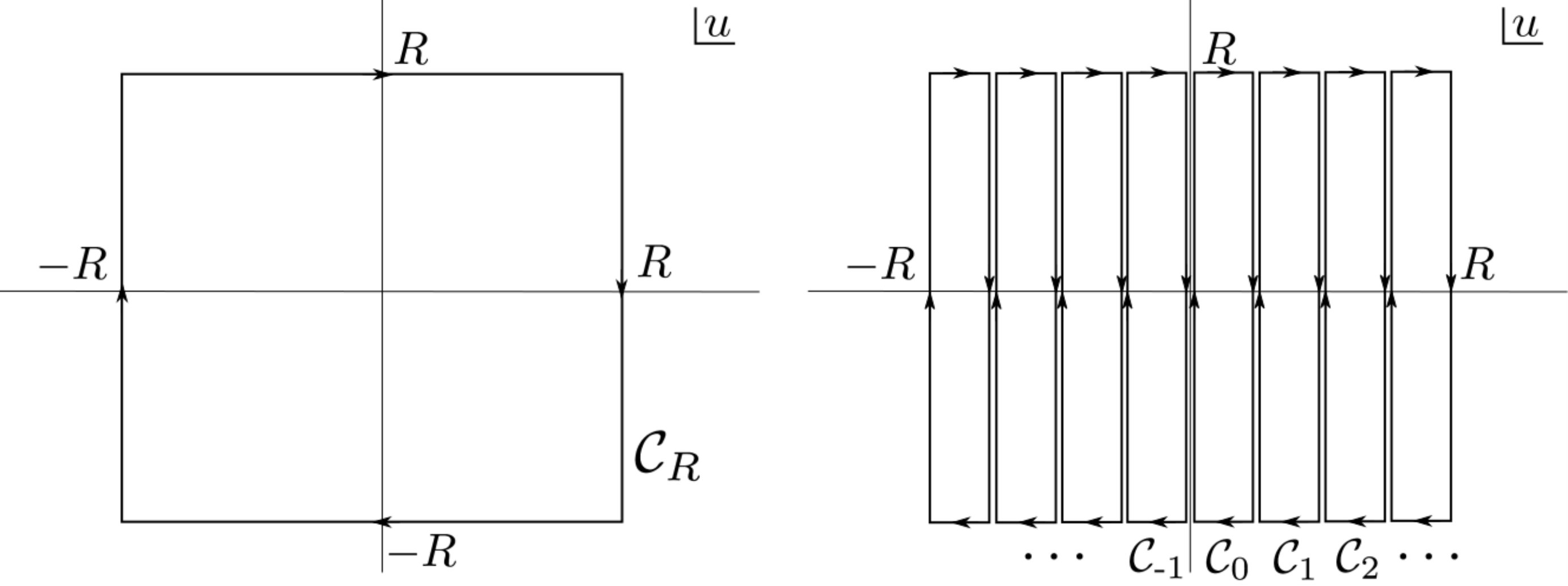 Figure 1
 Figure 2
 Figure 3
 Figure 4
 Figure 5
 Figure 6
 Figure 7
 Figure 8
|
|
|
|
|
|
|
|
|
|||||||||||||||||
| - |
|
|
|
|
|
|
|
|||||||||||||||||
| - | - |
|
|
|
|
|
|
|||||||||||||||||
| - | - | - |
|
|
|
|
|
Peer Reviews
No public reviews on file for this paper yet. If you reviewed it on a platform where reviews are public (OpenReview, ICLR, NeurIPS, ICML), you can paste yours below so the community can read it here.
Videos
No videos yet. Explain this paper in a talk, walkthrough, or lecture? Add one.
Supersymmetric partition functions
and the three-dimensional A-twist
Cyril Closset,♭ Heeyeon Kim♯ and Brian Willett*♮*
*♭*Theory Department, CERN
CH-1211, Geneva 23, Switzerland
♯ Perimeter Institute for Theoretical Physics
31 Caroline Street North, Waterloo, N2L 2Y5, Ontario, Canada
♮ Kavli Institute for Theoretical Physics
University of California, Santa Barbara, CA 93106
Abstract:
We study three-dimensional supersymmetric gauge theories on , an oriented circle bundle of degree over a closed Riemann surface, . We compute the supersymmetric partition function and correlation functions of supersymmetric loop operators. This uncovers interesting relations between observables on manifolds of different topologies. In particular, the familiar supersymmetric partition function on the round can be understood as the expectation value of a so-called “fibering operator” on with a topological twist. More generally, we show that the 3d supersymmetric partition functions (and supersymmetric Wilson loop correlation functions) on are fully determined by the two-dimensional A-twisted topological field theory obtained by compactifying the 3d theory on a circle. We give two complementary derivations of the result. We also discuss applications to F-maximization and to three-dimensional supersymmetric dualities.
Supersymmetry, Topological Field Theory
††preprint: CERN-TH-2017-006
Contents
-
2.5 Partition function and loop-operator correlation functions
-
2.6 Gauging flavor symmetries and the on-shell twisted superpotential
-
6.1 Two-term dilogarithm identities and abelian mirror symmetry
1 Introduction
Supersymmetric partition functions are useful to explore strongly-coupled theories with various amounts of supersymmetry—see e.g. [1, 2, 3, 4, 5, 6]. This is particularly true in three dimensions, where there are fewer non-perturbative tools available than in even dimensions. For instance, in three-dimensional conformal field theories (CFT), the quantity
[TABLE]
where is the partition function on the round three-sphere, 111The log of the partition function is UV divergent; is defined as its finite piece upon taking the UV cut-off to infinity. is a fundamental quantity analogous to the central charge in even dimensions [7, 8, 9]. In three-dimensional theories with supersymmetry, we can often compute (1.1) exactly by supersymmetric localization in a gauge-theory UV completion of the CFT [2, 3, 4].
In this work, we consider gauge theories with an -symmetry . We study them on a three-manifold , a principal bundle over a Riemann surface:
[TABLE]
This family of geometries is indexed by two integers, , the genus of the Riemann surface , and , the first Chern number of the principal bundle. It includes the round three-sphere and the product spaces :
[TABLE]
We derive general formulas for the supersymmetric partition functions and for expectation values of supersymmetric Wilson loops (and other loop operators) wrapped on an fiber. We heavily exploit the fact that the supersymmetric background on is a pull-back of the two-dimensional topological A-twist on [10, 11]. Note that a very similar computation was performed in [12] for theories with supersymmetry. 222We differ from [12] in our treatment of fermionic zero-modes and obtain different results for .
An interesting upshot of our analysis is that the partition function can be viewed as the expectation value of a particular loop operator wrapped on in the topologically-twisted theory on —that is:
[TABLE]
We call the fibering operator. Its insertion along an fiber in corresponds to shifting the Chern number of the total space, replacing by . The relation (1.4) is a generalization to theories of a similar relation in Chern-Simons theory [13]. We will compute the fibering operator explicitly for supersymmetric Yang-Mills-Chern-Simons-matter theories. Note that the relation (1.4) only holds for theories with integer-quantized -charges, because the -charges are integer-quantized on . However, the result can be analytically continued to real -charges in a canonical fashion [4, 14].
In the rest of this introduction, we summarize our main results and discuss relations to previous works.
Seifert manifolds, three-dimensional -twist and the Coulomb branch
For 3d theories with an -symmetry, the three-dimensional backgrounds that allow for some supersymmetry were classified in [11]. In order to preserve two supercharges of opposite -charges, the three-manifold must admit a nowhere-vanishing Killing vector . There are two distinct possibilities:
- •
is real. Then must be an (orientable) Seifert manifold—an bundle over a two-dimensional orbifold .
- •
is complex and generates two isometries. The only known example is the “untwisted” background of [15]. The corresponding partition function computes the so-called superconformal index [16, 15].
In this work, we focus on the simplest supersymmetric Seifert-manifold backgrounds satisfying two additional conditions: 1) the orbits of are the Seifert fibers; 2) the base space is a smooth closed Riemann surface (without orbifold points).
Condition 1) could be waived in the case of a base with genus or . For , this corresponds to turning on a ‘squashing’ parameter—this is often denoted by on lens space backgrounds—see e.g. [17, 18, 19]. It will be essential to our story that we do not allow any such squashing deformation. Condition 2) is not essential to our story but it is assumed for simplicity. We hope to report on the case of general Seifert manifolds in future work.
These two conditions imply that the supersymmetric background on is a pull-back of the ordinary A-twist for two-dimensional theories on the Riemann surface . 333Strictly speaking, this is for a particular choice of the “shift by ” in [11]. See Appendix B. In this language, localization on becomes a simple generalization of a recent localization computation on [20, 21, 22].
As we will show, the supersymmetric partition functions on the A-twisted can be constructed in terms of the low-energy theory on the Coulomb branch of the flat-space theory on . We may view the three-dimensional theory on a circle of radius as a two-dimensional supersymmetric theory with an infinite number of fields. This theory has a classical Coulomb branch spanned by the coordinates , where is the real scalar in the 3d vector multiplet and is the holonomy of the gauge field on (along the Cartan of the gauge group). The low-energy dynamics on the Coulomb branch is governed by the effective twisted superpotential . We will discuss this function in depth, paying particular attention to the effect of the Chern-Simons terms. Schematically, it is given by:
[TABLE]
The first term is the gauge CS term, the second term is a gravitational CS term, and the last term is the contribution of chiral fields with gauge charges . Note that we assign a physical significance to the constant piece of , which is identified with the gravitational CS level in three dimensions.
The coupling of this effective theory to curved space is governed by the so-called effective dilaton, which takes the schematic form:
[TABLE]
Here and are mixed -gauge and CS levels, respectively. The other terms are the contribution of the chiral multiplets (with -charges ) and of the W-bosons. These two functions were derived in [23, 24]; in addition, we included the contribution of the and gravitational supersymmetric CS terms of [25].
From (1.5) and (1.6), we construct two well-defined Coulomb-branch operators. The handle-gluing operator is given by [24]:
[TABLE]
It corresponds to adding a handle to the base , shifting to . The fibering operator introduced above is a simple function of the twisted superpotential:
[TABLE]
This is our main result. The formula (1.8) will be made more precise in the main text.
Consider a theory such that the “Bethe vacua” (the abelian Coulomb branch vacua, which are the gauge-inequivalent solutions to the Bethe equations [26] of the theory) are distinct. This always happens, for instance, in theories with enough flavor symmetries and with generic fugacities. In that case, the find the simple result:
[TABLE]
with the set of Bethe vacua. For , this is the so-called twisted index on [24, 21, 22]. In particular, the partition function on computes the 3d Witten index studied in [27]. For , , on the other hand, we have the familiar partition function, and the relation (1.4) directly follows. More generally, we have:
[TABLE]
for the expectation value of a supersymmetric Wilson loop wrapped on the fiber. We do not specify the insertion points on since the 2d theory is topological. We may view and as particular defect loop operators in the 3d gauge theory, given by (1.7) and (1.8) on the Coulomb branch.
Localization formula
Another formula for the partition function can be obtained by supersymmetric localization in the UV. We follow the abelianization method of Blau and Thompson [28, 13] adapted to the supersymmetric context. From that point of view, the partition function for can be written as:
[TABLE]
The sum is over flat torsion bundles for the Cartan subgroup of the gauge group . The meromorphic integrand contains classical contributions (the Chern-Simons terms and FI parameters) and one-loop contributions from all the matter fields. The contour integral is taken along a particular “Jeffrey-Kirwan (JK) contour” on a multiple cover of the Coulomb branch (with ). Using gauge invariance, one may also write (1.11) as:
[TABLE]
where the sum is over all GNO-quantized fluxes of , while the variables are gauge-fixed to . The expression (1.12) is also valid at [21, 22], in agreement with the relations (1.10). By resuming the fluxes in (1.12), one can obtain the Bethe-vacua formula (1.9). Here we should note that we only rigorously derived the JK contour in (1.11) or (1.12) in the rank-one case. The higher-rank formula should be considered as a well-motivated conjecture. (It also follows in good part from earlier results relating supersymmetric localization [29, 30, 20, 31] to JK residues [32, 33].)
For , the JK contour in (1.11) can be deformed to a simple “-contour” which lies along the imaginary axis—that is, we have an integral over real :
[TABLE]
in some appropriate region of parameter space. This is the familiar integral over real on [2]. For generic fugacities, the contour along generally has to be deformed, so that it always “separates” the singularities of the integrand in the same way. For pure supersymmetric Chern-Simons theory, we may also rotate the contour to lie along the real axis in the plane; such a theory is equivalent to ordinary Chern-Simons theory (up to a shift of the CS level), and (1.13) indeed reproduces the known integral formula over the holonomies in that case [13].
Parity anomalies, contact terms and Chern-Simons levels
As is well known, a three-dimensional Dirac fermion coupled to gauge fields suffers from the so-called parity anomaly; one cannot quantize the fermion while preserving both gauge invariance and three-dimensional parity [34, 35, 36]. Throughout this work, we choose a gauge-invariant regularization of the 3d chiral multiplet. After integrating out the matter fields, the lack of parity invariance of the vector multiplet effective action (both for dynamical gauge fields and background gauge fields for global symmetries) is encoded in certain parity-odd contact terms in two-points functions of the corresponding conserved currents. We denote these contact terms by . Unlike ordinary contact terms, which are generated by local terms in the effective action and are therefore ambiguous, the contact terms correspond to Chern-Simons terms in the action, whose couplings —the CS levels—are integer-quantized for compact gauge groups. The contact terms , therefore, are physically meaningful modulo integer shifts, [25]. In this work, we are careful in distinguishing between and . Unless otherwise specified, the CS levels are always integer-quantized, while chiral multiplets contributes certain half-integers to . For instance, a single chiral multiplet coupled to a (background) gauge field with charge will be quantized with a contact term for that . This is sometimes referred to as a “ quantization”.
This distinction is not only pedantic. It is crucial in order to compute partition functions, including all dynamical and background Chern-Simons terms, in a consistent manner. This resolves some confusions about “sign ambiguities” that appeared in [20, 21, 22]—there are no sign ambiguities except for the ones encoded in CS terms for global symmetries. Relatedly, we will correct some signs that arise from classical CS actions for abelian gauge groups. (See in particular Appendix C.)
Dualities and on-shell superpotential
Many 3d supersymmetric gauge theories are related by infrared dualities. On general grounds, the partition function (and other supersymmetric observables) of two dual theories and should agree on any supersymmetric background:
[TABLE]
The Bethe-vacua formula (1.9) for is particularly convenient to check these duality relations. The duality relations (1.14), and similar relations for loop operator insertions, can be rephrased as a statement about matching Bethe vacua in a one-to-one fashion. The duality statement is that the handle-gluing and fibering operators of the dual theories agree “on-shell”, that is, when evaluated on a dual pair of Bethe vacua, and .
Equivalently, one can state the duality relations in terms of the effective twisted superpotential: The twisted superpotentials of the dual theories must agree on-shell:
[TABLE]
on any pair of dual vacua 444The twisted superpotential suffers from branch-cut ambiguities, and this relation holds for a particular choice of branches. (and similarly for the so-called on-shell effective dilaton, that we will define later). Interestingly, the relations (1.15) for gauge-theory dualities often follow from known dilogarithm identities [37]. We should emphasize that, even in the case of the partition functions, this provides a simpler derivation of the duality relation (1.14) than previous investigations of complicated integral identities—see in particular [38, 39, 40]. 555On the other hand, those integral identities are valid on with non-zero squashing, , while we only consider .
We will also discuss how we can use the on-shell twisted superpotential to gauge a flavor symmetry, independently of whether the original theory has a Lagrangian description.
Relation to previous works and outlook
The three-dimensional A-twist vantage point relates the partition function [2, 3, 4] with the twisted indices [20, 21, 22]. As already noted, this generalizes known results for pure CS theories [13] to supersymmetric gauge theories with matter. This framework also explains the results of [41] on the Wilson loop quantum algebra on , which is encoded in the Bethe equations [22]. A similar relation between the twisted index and the partition function was also observed in large quiver gauge theories [42, 43].
For generic values of , the supersymmetric background only allows for quantized -charges. When , including the case , on the other hand, the -charges can be varied continuously. We will explain how our formulas for can account for any -charge, in those cases. On , this allows us to probe properties of the infrared CFT, where the -charges are generally irrational. Whenever the UV -symmetry can mix with abelian flavor symmetries along the RG flow (and in the absence of accidental symmetries), the superconformal -charge in the infrared can be determined by -maximization [4, 44]. That is, we need to maximize (1.1) over the possible trial -charges. Our Bethe-vacua formula for is well-suited for this computation, and the results compare well with previously-obtained results using the integral formula (1.11).
Another important localization result available in the literature is the lens space partition function [45, 46]. We should note that the supersymmetric background for the manifold:
[TABLE]
that we consider here, is distinct from the background considered in [45, 46, 47], if . The main difference between the two supersymmetric backgrounds is that the -symmetry line bundle present on (1.16) is topologically non-trivial, unlike the background of [45, 46].
In the A-twist language, the background corresponds to a genus-zero Riemann surface with two orbifold points. We hope to address this case in future work, along with generic Seifert manifolds. Pure Chern-Simons theory on a restricted class of Seifert manifolds was considered in [48, 49].
The formula (1.9) for the supersymmetric partition functions is reminiscent of the surgery prescription for pure CS theory [50]. Here we have a potentially richer quasi-topological structure that depends holomorphically on various parameters. It would be very interesting to explore that point of view further.
Another construction of supersymmetric partition functions is in terms of holomorphic blocks [51]. They are partition functions on , with a disk, which are in one-to-one correspondence with the Bethe vacua. Despite the similarities, that approach seems somewhat orthogonal to the one of the present paper, especially since the squashing parameter (or -deformation on ) plays such an important role in [51], while we set it to zero throughout. Nonetheless, it would be very interesting to understand better the relation between the two approaches. Relatedly, our results should be of interest in the context of the 3d/3d correspondence [52, 53, 54]. In particular, one might ask what kind of topological field theory can be obtained by compactifying M5-branes on the supersymmetric background ; progress on understanding such systems has been made recently in [55, 56].
Finally, let us mention that results completely analogous to the ones of this paper can be obtained for four-dimensional theories on [57].
This paper is organized as follows. In Section 2, we explore the two-dimensional A-model point of view and we derive the Bethe-vacua formula (1.9). In Section 3, we summarize important aspects of curved-space supersymmetry on . In Section 4, we discuss supersymmetric localization and we obtain the localization formula (1.11). In Section 5, we compute the partition function with the Bethe-vacua formula, and we present some non-trivial examples of -maximization. In Section 6, we study the matching of supersymmetric partition function across gauge-theory dualities. Additional material is contained in various appendices.
2 The partition function as a sum over Bethe vacua
In this section, we start by reviewing some relevant results about two-dimensional gauge theories. We then consider three-dimensional gauge theories on a circle as a two-dimensional theory and discuss in detail the low-energy theory on the Coulomb branch. We argue that the partition function on can be obtained as a sum over “Coulomb branch vacua” (Bethe vacua) by a simple modification of the formula for the twisted indices discussed in [24, 22, 21]. We will give a microscopic derivation of this result in Section 4.
2.1 The Bethe-vacua formula in two dimensions
As a preliminary, consider a two-dimensional gauge theory with gauge group and chiral multiplets in representations of . From the vector multiplet , one can build a -valued twisted chiral multiplet with components:
[TABLE]
Here we follow the A-twist conventions of [31]. In particular, the gauginos , are - and -forms after the twist, respectively. 666To avoid any possible confusion, let us recall that there are two distinct but standard usages of the term “twist” in two dimensions. The terms “twisted chiral multiplet” and “twisted mass” refer to representations of supersymmetry, while the “A-twist” is a topological twist of the theory. See also Appendix B.
Let us denote by the flavor symmetry group (the non-R global symmetry group) of the theory. It is natural to couple the flavor currents to a background vector multiplet . The so-called twisted masses corresponds to constant expectations values for its complex scalar component. A particular chiral multiplet has twisted mass , where is a weight of the flavor representation.
At a generic point on the classical Coulomb branch, the gauge group is broken to the Cartan subgroup , and the massive chiral multiplets and W-bosons can be integrated out. The low-energy dynamics on the Coulomb branch is governed by the effective twisted superpotential [58, 23, 26]:
[TABLE]
The first term in (2.2) is the contribution from the two-dimensional complexified Fayet-Iliopoulos (FI) parameters, with a projection on the free abelian subgroup . The second term in (2.2) is the contribution from the chiral multiplets , with the weights of the representation . The last term in (2.2) is the contribution from the W-bosons and their superpartners, with a sum over the positive roots of .
In the following, it will be useful to pick a basis of the Cartan of , and a basis of the Cartan of , such that:
[TABLE]
We choose a basis that generates the coweight lattice , so that for all weights , and similarly for the flavor group.
We view the low energy theory on the Coulomb branch as an A-twisted Landau-Ginzburg (LG) model [59] with twisted superpotential for the twisted chiral multiplets . However, we see from (2.1) that the highest component of is an abelian field strength. We may treat as the fundamental variable if we also impose flux quantization by hand [26]:
[TABLE]
on any compact space. Relatedly, the twisted superpotential (2.2) suffers from branch cut ambiguities due to the logarithms:
[TABLE]
The quantization condition (2.4) ensures that (2.5) only shifts the effective action by an integer multiple of , so that the path integral remains well-defined. When looking for the vacua of the theory, we have to take the ambiguity (2.5) into account. This leads to the so-called Bethe equations [26]:
[TABLE]
Note the left-hand side is independent of the branch-cut ambiguity—in fact, it is a rational function of and .
If is abelian, the solutions to (2.6) correspond directly to the vacua of the theory. In a non-abelian theory, we must divide by the action of the Weyl group of , . In addition, solutions which are not acted on freely by the Weyl symmetry correspond to putative vacua with unbroken non-abelian gauge symmetry, wherein the derivation of (2.2) is unreliable. Following [60], we will exclude these solutions, which are believed not to correspond to physical vacua. (See also [61] for a related recent discussion.) Thus the set of vacua of the Coulomb branch theory is given by: 777For simplicity in this paper, we consider compact connected gauge groups, such that the Weyl group of and the Weyl group of its Lie algebra coincide. Then the condition , is equivalent to , .
[TABLE]
We refer to the solutions (modulo the Weyl symmetry) as the “Bethe vacua”.
2.1.1 Coulomb branch correlation functions
The Coulomb branch operators are the twisted chiral ring operators given by gauge-invariant polynomials in the scalar field . On the classical Coulomb branch, they correspond to Weyl-invariant polynomials in the variables . The effective twisted superpotential provides us with twisted chiral ring quantum relations.
Let us consider the theory on a closed orientable Riemann surface with the topological A-twist. The low energy topological field theory for the twisted chiral multiplets has an effective action:
[TABLE]
up to -exact terms. The first term in (2.8) depends on the effective twisted superpotential , and it is explicitly topological (since and are naturally 2-forms). The second term involves the Ricci scalar, and it is topological for the constant modes of due to the Gauss-Bonnet theorem. It corresponds to the “improvement” Lagrangian of [62]. The holomorphic function is the effective dilaton which governs the coupling of the theory to the A-twist background. In our two-dimensional gauge theory, it is given by [23, 24]:
[TABLE]
up to an arbitrary constant. Here denote the -charges of the chiral multiplets , which should be integers so that the theory can be defined on any .
The correlation functions of Coulomb branch operators can be computed as a sum over the Bethe vacua, by a direct generalization of Vafa’s formula for ordinary topological LG models (LG) [59]. One finds [24]:
[TABLE]
with
[TABLE]
the so-called handle-gluing operator. The first factor in (2.11) comes from the last term in (2.8) evaluated on the Coulomb branch, and the Hessian determinant of the superpotential arises because of the gaugino zero-modes on . One can also obtain (2.10) by supersymmetric localization in the UV [21].
There is an important caveat to this discussion: we have assumed that the Bethe vacua are isolated. This generally happens in theories with enough flavor symmetries and with generic twisted masses. Many important two-dimensional theories do not satisfy this condition, however—for instance, any GLSM that flows to a Calabi-Yau NLSM in the IR has a degenerate ; on the other hand, such theories can still be studied by localization methods, at least at genus [63, 31]. Isomorphic comments apply in three dimensions.
2.1.2 Flux operators
In the presence of a flavor symmetry group , it is natural to turn on supersymmetric background fluxes for the gauge field in ,
[TABLE]
in addition to the twisted masses . This adds a term:
[TABLE]
to the topological effective action (2.8). We are free to choose the background gauge field at will. In particular, we may consider the addition of a -function flux at a point on :
[TABLE]
for each . In this case, we have:
[TABLE]
Therefore, the insertion of a unit of background flux on can be viewed as the insertion of a local operator at . We will call such operators the flux operators.
Incidentally, the handle-gluing operator (2.11) can itself be thought of as a flux operator for the vector-like -symmetry. On the A-twist background, the -symmetry background flux is:
[TABLE]
in order to preserve supersymmetry. Therefore, adding a handle has the same effect as adding one unit of flux.
2.2 Three-dimensional gauge theories on a circle
Let us now consider a three-dimensional supersymmetric gauge theory compactified on a circle of radius . We view this theory as a two-dimensional theory with an infinite number of fields, corresponding to the Kaluza-Klein (KK) modes of each three-dimensional field.
At finite , the complex scalar in any vector multiplet is cylinder-valued due to large gauge transformations. We introduce the notation:
[TABLE]
for the scalar fields in the Cartan of . Here and are real scalars in 3d vector multiplets, and denotes the holonomy along . We have the identifications and under large gauge transformations. The dimensionless quantity in (2.17) is related to the two-dimensional complex scalar of Section 2.1 by . It is often convenient to work with the single-valued fugacities:
[TABLE]
The low energy theory on the Coulomb branch (with coordinates ) is still governed by the topological effective action (2.8), but the twisted superpotential and the effective dilaton have new features intimately related to three-dimensional physics. In the following, it will be convenient to rescale according to , so that both and are dimensionless quantities.
2.2.1 The three-dimensional twisted superpotential
The classical part of the twisted superpotential is related to Chern-Simons interactions in three dimensions. Consider any vector multiplet. A Chern-Simons interaction with level contributes to the twisted superpotential as:
[TABLE]
This can be derived by direct evaluation of the Chern-Simons functional on , for instance, as we will explain in Section 4. The quadratic piece is essentially a mass term, corresponding to the well-known fact that the CS interaction lifts the three-dimensional Coulomb branch classically. The linear piece in (2.19) is related to the subtle signs alluded to in the introduction (see also Section 4 and Appendix C). Although this is not single-valued, it may only shift by terms of the form (2.5), which do not affect the path-integral. For future reference, we may rewrite (2.19) as a function of :
[TABLE]
with a branch cut along the positive real axis . (Here the is on its principal branch, so that .)
Similarly, a mixed CS term between and contributes:
[TABLE]
In addition, we claim that the supersymmetric gravitational Chern-Simons term [25] contributes a constant term:
[TABLE]
with . We will give several justifications for this claim below. In total, the contribution of all the gauge, flavor and gravitational CS terms to the twisted superpotential read:
[TABLE]
where all the levels are integer-quantized. For any simple group , we have with the Killing form of (and running over its Cartan subgroup).
Consider next the one-loop contribution of the three-dimensional chiral multiplets. A chiral multiplet with charge under some symmetry contributes:
[TABLE]
with the effective twisted mass of and ; the symmetry could be dynamical, flavor or a combination of both. The first equality in (2.24) gives as a formal sum over KK modes. Upon regulating that expression, we obtain the dilogarithm of . As we will explain in Section 4, we have implicitly chosen a regularization scheme that preserves gauge invariance at the expense of “parity”. This is often stated as a “ quantization” of the chiral multiplet, wherein we turn on a “half-integer CS level to cancel the parity anomaly”. In this work, we never consider “half-integer” CS levels since they are not well-defined. The quantization of the chiral multiplet implicit in (2.24) is gauge-invariant and includes a contact term for the current two-point function [25]. We also have a gravitational contact term . The only scheme ambiguity is in shifting by an integer CS level (and by an integer ), corresponding to
[TABLE]
which would correspond to a “ quantization”. An important consistency check of the twisted superpotential (2.24) is that it reproduces the correct decoupling limits at large value of the three-dimensional real mass . We have:
[TABLE]
which corresponds to the expected shift of the contact terms:
[TABLE]
For large positive , we obtain an empty theory and the twisted superpotential vanishes, while at large negative we are left with the background and gravitational CS levels and , as we can see by comparing (2.26) to (2.20) and (2.22). This gives a first consistency check of the detailed form of (LABEL:WCS_gen). We can easily generalize this consistency check to chiral multiplets coupled to arbitrary background gauge fields. We refer to Section 4.3.2 for additional discussions of our treatment of the chiral multiplets.
As another consistency check, let us consider a pair of two chiral multiplets , of charges . Since this allows for a superpotential mass term , the low energy theory should be empty. More precisely, it is empty if we consider two multiplets with opposite contact terms, which amount to adding CS level and , with our choice of quantization. We then have:
[TABLE]
Here we have used the dilogarithm identity:
[TABLE]
In Section 6, we will relate other dilograrithm identities to non-trivial dualities between different gauge theories.
Finally, we should consider the effect of the W-bosons and their superpartners on the Coulomb branch, which contribute like chiral multiplets of gauge charges and -charge . For every pair of roots , we choose the “symmetric” quantization, with opposite contact terms for and . Therefore, due to the identity (2.29), the W-bosons do not contribute at all to the effective twisted superpotential in three dimensions.
For general Chern-Simons-Yang-Mills matter theories with gauge group and chiral multiplets in representations of , we have the twisted superpotential:
[TABLE]
where the classical contribution is given by (LABEL:WCS_gen). Here we introduced the short-hand notation:
[TABLE]
where is the flavor charge of (that is, a weight of the flavor group). Note that this twisted superpotential is only defined modulo the branch-cut ambiguities:
[TABLE]
However, all the physical observables that we will define are free from such ambiguities.
2.2.2 Flux operators and Bethe equations
As in two dimensions, we may define the flux operators:
[TABLE]
for the gauge and flavor symmetries, respectively. This is obviously invariant under (2.32). One can check that these operators are rational functions of the fugacities and . The three-dimensional flux operators are loop operators supported along the direction. They can be identified with the vortex loops discussed in [64, 65]. The Bethe vacua are given by:
[TABLE]
In particular, they are rational equations for the single-valued variables .
2.2.3 The effective dilaton and the handle-gluing operator
If we couple the 3d theory to a background with the A-twist along , the effective dilaton can be computed like in two dimensions [24]. As we will further discuss in Section 4, the classical Chern-Simons terms for the background gauge field [25] contributes:
[TABLE]
Here , denote mixed -gauge and -flavor CS levels, and is the CS level. All these levels are integer-quantized. A chiral multiplet of gauge charge and -charge contributes:
[TABLE]
This corresponds to the same “ quantization” discussed above, which includes the contact terms and for the gauge- and - conserved-current two-point functions, respectively. The limits
[TABLE]
reproduce the correct shifts of the CS terms upon integrating out a chiral multiplet. 888That is, taking into account that is only defined modulo an integer. The second limit in (2.37) corresponds to CS levels and . The W-bosons contributes similarly like chiral multiplets of -charge . Due to our choice of “symmetric quantization” mentioned above, we also have a shift of by .
In total, the effective dilaton of our 3d supersymmetric gauge theory compactified on reads:
[TABLE]
with the -charge of . The three-dimensional handle-gluing operator is given by:
[TABLE]
This directly leads to an expression for the twisted index as a sum over Bethe vacua [24, 22, 20]. Note that we accounted for the effect of the CS level in (LABEL:Omega_full). This leads to a subtle sign in (2.39), which was previously overlooked.
2.3 Induced charges of monopole operators
For future reference, let us consider the induced charges of the bare monopole operators . These operators are associated with the limit on the classical Coulomb branch. We define their induced charges by:
[TABLE]
for their gauge, flavor and -charges, respectively. One can easily check that these formula reproduce the standard one-loop formula for the induces charges; see e.g. [22]. By construction, the charges (LABEL:induced_charges_T) are always integers.
2.4 The fibering operator in three dimensions
In addition to the three-dimensional flavor symmetry group , the effective two-dimensional theory has a symmetry whose charge is the KK momentum. We may turn on a supersymmetric background vector multiplet for . It originates from the three-dimensional “new-minimal” supergravity multiplet—see e.g. [25, 66]—which decomposes into a supergravity and a vector multiplet upon KK reduction to two dimensions. The twisted mass associated to is . Indeed, the twisted masses for the KK tower of any 3d chiral multiplet takes the form , with the KK momenta.
In any three-dimensional theory, there must exist a distinguished flux operator for , which we denote by . The insertion of at a point on has the effect of introducing one unit of flux for , which is nothing but a shift of the first Chern class of the principal bundle over . In particular, the partition function of can be written in terms of insertions of on :
[TABLE]
Since introduces a non-trivial fibration of the circle over , we call it the fibering operator. Reinstating dimensions, we have:
[TABLE]
with the dimensionless given by (2.30). This gives us the explicit form of the fibering operator for any 3d gauge theory:
[TABLE]
We immediately see that (2.43) is insensitive to the branch-cut ambiguities (2.32) of the twisted superpotential. On the other hand, it transforms non-trivially under large gauge transformations or (for either the gauge or flavor group). We find:
[TABLE]
where are the flux operators defined in (2.33).
2.4.1 The Chern-Simons and chiral multiplet fibering operator
For future reference, we note that the effect of the classical CS terms (LABEL:WCS_gen) on the fibering operator is:
[TABLE]
Similarly, a chiral multiplet of charge under some contributes:
[TABLE]
This defines a meromorphic function of on the complex plane, as the branch cuts of the dilogarithm and logarithm cancel each other. The function (2.46) has poles of order at , and zeros of order at , . (This is proven e.g. by proposition 5.1 of [67].) It is closely related to the chiral multiplet one-loop determinant on , as we discuss further in Section 5.1.
We note that the Chern-Simons and chiral fibering operators satisfy:
[TABLE]
where “” denotes all Chern-Simons levels and contact terms in the theory, including the gravitational Chern-Simons level and the contact terms appearing in the quantization of the chiral multiplet. This operation thus has the same effect as taking . As discussed further in Section 4.3.2, this reflects the fact that the and backgrounds are related by a parity transformation.
2.5 Partition function and loop-operator correlation functions
Combining all the ingredients introduced so far, we can write the supersymmetric partition function on as:
[TABLE]
Here we introduced generic background fluxes for the flavor symmetry. As we discussed, we can also view these background fluxes as inserting flux operators at points on . (A constant background flux is then viewed as a “smeared” flux operator.) Note that, in the presence of any abelian flavor symmetry , we may shift the -symmetry by , where is quantized to preserve the Dirac quantization of the -charge. The net effect on the partition function is to shift the background flux . This amounts to a shift:
[TABLE]
in the topological effective action (2.8). The partition function (2.48) is unaffected if we shift the -symmetry current by any abelian gauge current.
We are also interested in supersymmetric Wilson loop operators along the fiber. Any such Wilson loop correspond to a Weyl-invariant Laurent polynomial in the fugacities ,
[TABLE]
For a Wilson loop in a representation of , we have:
[TABLE]
where the fiber coordinate. We then have the expectation value:
[TABLE]
From this formula, we can read off the quantum algebra of Wilson loops, which is an uplift of the 2d twisted chiral ring [41, 22]. The quantum relations are the relations satisfied by solutions to the Bethe equations (2.34).
Let us briefly comment on the defect operators . They enter in (2.52) in the same way as the Wilson loops, in agreement with their interpretation as operators supported along at a particular point on the base . These line operators can be identified with the vortex loop operators discussed in [64, 65]. In principle, one can insert fractional flux at points on as long as the total flux is integer. The effect of such operators is to impose that matter fields charged under the flavor symmetry induce a non-trivial holonomy as they wind around the vortex loop. The Bethe equations imply relations satisfied by flux operators, just like for Wilson loops.
2.6 Gauging flavor symmetries and the on-shell twisted superpotential
Given a flavor symmetry, it is natural to gauge it, by promoting background vector multiplets to dynamical ones. This is an important operation for producing new theories from old ones, and we would like to perform it at the level of the partition function (2.48). This can be done most conveniently by working with the “on-shell” effective twisted superpotentials and effective dilatons,
[TABLE]
which are evaluated at solutions to the Bethe equations. The functions (LABEL:Wonshell) are particularly useful because we can use them to construct all of the ingredients in the partition function (2.48), even if one does not have access to a Lagrangian description of the theory.
As described above, the supersymmetric vacua of the theory are determined by solutions to the Bethe equation (2.34). For generic-enough mass parameters , this has a finite number of solutions,
[TABLE]
It is important to stress that the functions generically have branch points, where two or more solutions become equal, and branch cuts, where the solutions are permuted. Thus it is more natural to think of as functions on an -fold branched cover of the space of the ’s.
To any Bethe vacua, we may associate the “on-shell” effective twisted superpotential and effective dilaton (LABEL:Wonshell), which we consider as a function on the -fold branched cover of the parameter space. Nonetheless, the twisted superpotential is not yet well-defined due to branch cut ambiguities of itself. To partially fix this ambiguity, we impose a “physical branch” condition:999Namely, the Bethe equation, (2.34), only imposes that the RHS is an integer, however, by “changing the branch” by adding appropriate integer multiples of to , we may arrange that the RHS is precisely zero.
[TABLE]
This function will still have branch cut ambiguities associated to the background gauge multiplets, i.e., it is defined only up to shifts , , but it will not have any branch cuts associated to shifts by the dynamical gauge field. This must be the case, as the dynamical gauge field should play no role in the low energy effective theory. Up to these shifts, the on-shell effective twisted superpotential is a physically-meaningful observable of the low-energy theory. In particular, it should match across dualities. Similar statements hold for the on-shell effective dilaton.
If one has access to the on-shell effective twisted superpotentials of a theory, one may construct the on-shell flux and fibering operators, even if the theory lacks a known Lagrangian description. They are given by:
[TABLE]
We can easily see that this agrees with the gauge-theory definitions (2.33) and (2.43) upon using (2.55). Similarly, the on-shell handle-gluing operator is simply defined by:
[TABLE]
which obviously agrees with (2.39).
Using the on-shell twisted superpotential, it is straightforward to gauge a flavor symmetry. For instance, suppose we want to gauge a subgroup of the flavor group , with parameters . We simply write the Bethe equation for in terms of , namely:
[TABLE]
These equations should be solved for each , and may have zero, one, or several solutions for each . The vacua of the new gauge theory is the union of these solutions for all , and the resulting on-shell twisted superpotential can be used to construct the partition function of the new theory. This procedure is described in more detail in Appendix E. We will see an example of this procedure in Section 6.
3 -twisted supersymmetric theories on
In this section, we study curved-space rigid supersymmetry on . We introduce a particular three-dimensional supergravity background which realizes the “three-dimensional A-twist” in a precise sense. We also discuss curved-space supermultiplets and Lagrangians on this background, following the general results of [11, 19].
3.1 Supersymmetric background on
Consider the three-manifold , a principal bundle of first Chern number over a closed oriented Riemann surface of genus :
[TABLE]
This is a simple example of a Seifert fibration. The topology of is fully specified by the two integer and . In particular, if we have the second cohomology:
[TABLE]
which includes the torsion subgroup . A more detailed account of the topology and geometry of is provided in Appendix A. Let us consider the metric
[TABLE]
with the fiber coordinate, and a complex coordinate on the base (in a given patch). The principal bundle connection has field strength:
[TABLE]
We normalize the volume of the base to , so that has flux
[TABLE]
on . The metric (3.3) admits a Killing vector whose orbits are the fibers. The dual one-form determines a transversely holomorphic foliation (THF) of . We define:
[TABLE]
Note that . We also define the tensor:
[TABLE]
which acts as a three-dimensional ‘complex structure’. (We summarize important aspects of this geometric structure in Appendix A.) The complex coordinates introduced above are coordinates adapted to the THF.
In order to preserve half of the flat-space supersymmetry on , we turn on additional background fields in the three-dimensional ‘new minimal’ supergravity multiplet [68, 69, 11]. This includes a scalar and a gauge field :
[TABLE]
with the metric determinant. The complete supergravity background is spelled out in Appendix B. The expression for in (3.8) is only valid in the adapted coordinates . Let us also define the adapted frame:
[TABLE]
Any one-form can be decomposed into ‘vertical’, ‘holomorphic’ and ‘anti-holomorphic’ components:
[TABLE]
and similarly for any tensor. (In the following, we will mostly use the frame basis.) The holomorphic component in (3.10) transforms as a section of a “canonical line bundle” on , denoted by , which is the pull-back of the canonical line bundle on the Riemann surface through the projection in (3.1). Its first Chern class is given by:
[TABLE]
where is the torsion subgroup in (3.2). It is very natural to introduce a modified Levi-Civita connection that preserves the decomposition (3.10). Following [11], we define the modified spin connection:
[TABLE]
with the standard spin connection. In particular, we have:
[TABLE]
The price to pay is that the modified connection has torsion, with the torsion tensor proportional to .
The supergravity background (3.3)-(3.8) preserves two (generalized) Killing spinors and , of -charge and , respectively, which satisfy:
[TABLE]
with given above. The holonomy of the modified connection is contained in , therefore it can be “twisted” away by a compensating transformation. The Killing spinors are then essentially constant in the adapted frame:
[TABLE]
This is the three-dimensional version of the A-twist. Geometrically, it corresponds to choosing the line bundle such that:
[TABLE]
This is a torsion line bundle with first Chern class:
[TABLE]
with the connection given by (3.8). It follows that the -charges must be integers in general. More precisely, we have the Dirac quantization condition:
[TABLE]
with the -charge of any field. Note that the bundle is topologically trivial if and only if . For instance, this is the case for the three-sphere .
The function in (3.8) and (3.15) corresponds to a gauge transformation. The Killing spinors (3.15) are globally well-defined if we choose . We may call this choice the “A-twist gauge”. More generally, we can choose a gauge , where is any integer; we will come back to this point below.
Note also that the Killing vector and the covector are built out of the Killing spinors (3.15) according to:
[TABLE]
with in our background. All the background fields are invariant under the isometry generated by . The compatibility condition (3.13) directly follows from (3.14) and (3.19).
3.1.1 Background vector multiplets
In addition to the background supergravity fields (3.3)-(3.8), we may also turn on background vector multiplets:
[TABLE]
for any flavor symmetry of the theory. To preserve the same supersymmetry as the geometric background, we take:
[TABLE]
a constant, which is the real mass associated to the flavor symmetry, and:
[TABLE]
with the field strength of and given in (3.8). This implies that is the connection of a holomorphic vector bundle over [19]. In particular, let us choose a holomorphic line bundle associated to a flavor symmetry. Its first Chern class has to lie in the torsion subgroup of the second cohomology (3.2):
[TABLE]
assuming . (See [22] for the case.) Let us also define:
[TABLE]
where is taken to be constant. The quantity (3.24) has a nice geometric interpretation as a complex modulus of the holomorphic line bundle [19]. Under a large gauge transformation along the circle fiber, the parameters and transform as:
[TABLE]
This must be an invariance of any physical observable.
3.1.2 vector multiplet
From the supergravity multiplet, one can also construct an abelian vector multiplet for the -symmetry [14]. In terms of the supersymmetric background (3.3)-(3.8), it is given by:
[TABLE]
where is the Ricci scalar of . In particular, one can check that the supersymmetry conditions (3.22) are satisfied:
[TABLE]
It follows that is a holomorphic line bundle, which is determined by its torsion flux (3.17) and by the modulus:
[TABLE]
Interestingly, is fully determined by the supergravity background. A large gauge transformation along the circle fiber corresponds to:
[TABLE]
Note that we can set , but it is sometimes useful to keep track of as a formal parameter, together with the gauge redundancy (3.29).
3.1.3 Parameter dependence and -charge dependence
Supersymmetric observables on depend explicitly on the discrete parameters and as well as on the torsion fluxes for flavor symmetries. They are also locally holomorphic functions of the complex parameters [19, 14]. Note that a line bundle generally has additional moduli, corresponding to flat connections along the one-cycles from . In our two-supercharge background, however, these additional moduli couple to -exact operators and supersymmetric observables are completely independent of them [19].
We can similarly understand the dependence of supersymmetric observables on the choice of -symmetry [14]. In a theory with abelian flavor symmetries, the -symmetry current can mix with flavor currents. Let us consider:
[TABLE]
for some parameter , which shifts the -charge by the charge according to . (The flavor charge is integer quantized by assumption.) This is equivalent to a shift of the vector multiplet by the vector multiplet:
[TABLE]
On our geometric background, the shift (3.30) is only allowed if it preserves the Dirac quantization condition (3.18). This implies that in general. On the other hand, if is topologically trivial (that is, if ), there is no restriction on the -charge and we can take . Geometrically, the shift (3.31) is a tensor product of line bundles:
[TABLE]
with integer or real, respectively. This corresponds to a shift of parameters:
[TABLE]
The partition function (or any supersymmetric observable) shifts accordingly. Note that the complex modulus stays invariant in the “-twist gauge” . This is the gauge that we used implicitly in Section 2. When is topologically trivial, another particularly interesting gauge is:
[TABLE]
In such a case, the dependence of supersymmetric observables on the -charge is entirely through the combination:
[TABLE]
with . Let us note that, in the case , the supersmmetric background considered in [2, 3, 4] has (setting for simplicity) and therefore the dependence on the -charge is holomorphic in the parameter [4, 14]. As we can see from (3.35), that property generalizes to any background admitting continuous -charges.
3.1.4 Comparison with three-sphere and lens space backgrounds
It is interesting to compare our family of curved-space backgrounds to the ones previously studied in the literature. The genus zero case, , corresponds to the lens space . For instance, we can consider the metric:
[TABLE]
with the angular coordinates and
[TABLE]
This is the total space of a degree bundle over the round , written down on the “northern patch” . 101010The usual Hopf coordinates are and , with . If we choose , we obtain the round metric on the quotient, and the remaining supergravity fields (see Appendix B) are:
[TABLE]
For , we can set by a large gauge transformation. This background is related to the three-sphere background of [2, 3, 4] by a so-called “ ambiguity” shift [11, 19] which we briefly discuss in Appendix B. While one can preserve four supercharges on , our background only preserves two of them.
For , we have a non-trivial holonomy of the -symmetry gauge field along the Hopf fiber, corresponding to the fact that . This is in contrast with the supersymmetric backgrounds considered in [45, 46, 47], which studied the same geometry (3.36) with a topologically trivial . The reason is that there exists two distinct supersymmetric backgrounds on the same topological space, corresponding to topologically distinct THFs. To explain this point, let us consider the lens space defined as the quotient of the three-sphere
[TABLE]
by the freely-acting action:
[TABLE]
with and two non-zero integers. The Hopf fibration considered above is given by the map:
[TABLE]
to the two-sphere, where is the complex coordinate on on the northern patch (), related to the angular coordinates above by . The quotient (3.40) acts on the base as:
[TABLE]
leaving it invariant if and only if (mod ). It follows that:
[TABLE]
as Seifert manifolds equipped with a particular THF. In contrast, the previous literature dealing with theories on lens spaces [45, 46, 47] considered instead. While and are homeomorphic, the THFs induced on them by the quotient (3.40) are distinct (if ). 111111The THFs are inherited from the complex structure on . A closely related statement is that there exists two distinct families of complex structures on the Hopf surface if [70], as discussed in [71]. We should note that the methods of this paper do not apply directly to or other lens spaces, because they would correspond to circle fibrations over the sphere with orbifold points. (These are examples of general Seifert fibrations, as mentioned in the introduction.) We also note that [12] studied gauge theories on the supersymmetric background.
3.2 Supersymmetric multiplets and Lagrangians
Given the supersymmetric background above, the supersymmetric multiplets and Lagrangians directly follow from the general results of [11]. In this subsection, we spell out those multiplets and Lagrangian in “A-twisted variables”—see Appendix B.1 and e.g. [31, 22]—in order to emphasize the relation to the A-twist on .
In the following, we write all the fields in the canonical frame basis. In that case, the holomorphic line bundle on is really a bundle, 121212We are being slightly cavalier in our notation since may denote either a holomorphic line bundle or the associated bundle: is a section of the holomorphic line bundle and is a section of the associated bundle. and . The corresponding charge is the “two-dimensional spin” of a field—in other words, a field of integer two-dimensional spin is a section of , and similarly for half-integer for some choice of square root. The three-dimensional A-twist (3.16) corresponds to a “twist” of the two-dimensional spin by the -symmetry according to:
[TABLE]
with the -charge. By definition, the A-twisted variables have vanishing -charge and definite twisted spins. Note that since is a torsion bundle. The real connection on is given by:
[TABLE]
with defined in (3.8). Let us also define the covariant derivative
[TABLE]
acting on tensors valued in , with and the connection defined by (3.12).
3.2.1 Supersymmetry algebra
The two Killing spinors (3.15) correspond to two supersymmetry transformations:
[TABLE]
which satisfy the supersymmetry algebra:
[TABLE]
Here is the real central charge of the superalgebra in flat space, and is the -covariant Lie derivative along the Killing vector . For a vector multiplet in Wess-Zumino (WZ) gauge, the real scalar component also enters (3.48) as , where is the actual central charge and is valued in the appropriate gauge representation. We should note that the Lie derivative and the covariant derivative coincide along , which means that:
[TABLE]
Note that we traded the -symmetry gauge field for in (3.48) since we are considering A-twisted fields, which are -neutral by definition.
3.2.2 Vector multiplet
Let and denote a compact Lie group and its Lie algebra, respectively. In WZ gauge, a -valued vector multiplet has components:
[TABLE]
The -twisted fermions decompose as:
[TABLE]
where the vertical components are scalar fields and the horizontal components , are sections of and , respectively. Let us define the field strength
[TABLE]
and denote by the covariant and gauge-covariant derivative. The supersymmetry transformations of (3.50) are
[TABLE]
The dependence of (LABEL:susyVector_twisted) on the geometric background is mostly implicit, through the covariant derivatives written in the frame basis. To check the supersymmetry algebra, it is important to note that:
[TABLE]
where appears due to the non-zero torsion of the covariant derivative.
3.2.3 Chiral multiplet
Consider a chiral multiplet of (integer) -charge , transforming in a representation of . In -twisted notation [31], we denote the components of by
[TABLE]
Similarly, the charge-conjugate antichiral multiplet of -charge in the representation has components
[TABLE]
The fields are valued in the canonical line bundle to the appropriate power. We have:
[TABLE]
where , are the gauge vector bundles. In particular, have two-dimensional spin , while have two-dimensional spin . The supersymmetry transformations of the chiral multiplet read:
[TABLE]
where is appropriately gauge-covariant and and act in the representation . We have:
[TABLE]
with defined in (3.45). For the antichiral multiplet, we similarly have:
[TABLE]
Using (LABEL:susyVector_twisted), one can check that (LABEL:susytranfoPhitwistBis) and (LABEL:susytranfotPhitwistBis) realize the supersymmetry algebra:
[TABLE]
where is the gauge-covariant Lie derivative, and acts in the appropriate representation of the gauge group.
3.2.4 Supersymmetric Lagrangians
To conclude this section, let us write down the most important supersymmetric Lagrangians for our three-dimensional gauge theories [11].
Vector multiplet.
The curved-space super-Yang-Mills (SYM) Lagrangian reads:
[TABLE]
Here and below, the trace over gauge indices is left implicit. The Lagrangian (LABEL:S_YM_full) is -exact, like any well-defined -term. One can check that:
[TABLE]
Another important Lagrangian is the Chern-Simons (CS) term. For any gauge group , we have
[TABLE]
with the CS level. 131313In general, we have a distinct CS level for each simple factor and for each factor in . In the presence of an abelian sector, we can also have mixed CS terms between and , with :
[TABLE]
with . For each factor, we may also turn on the Fayet-Iliopoulos parameter:
[TABLE]
where we normalized like in [22]. The FI term is a special case of a mixed CS term between the vector multiplet and the background vector multiplet (with real mass and vanishing flux ) for the associated topological symmetry , with level .
Chiral multiplet.
The standard kinetic term for a chiral multiplet coupled to a vector multiplet (in WZ gauge) reads:
[TABLE]
This Lagrangian is -exact:
[TABLE]
Finally, we may write down superpotential interactions in terms of a superpotential of -charge . Those interaction terms are -exact and do not play any crucial role in the following. The only way the superpotential appears in the localization computation is by the constraints it imposes on the flavor symmetry and -charges.
and gravitational Chern-Simons terms.
Three additional supersymmetric Chern-Simons Lagrangians are available in curved space [25, 11]. Let us consider them on our background.
The first Lagrangian is simply a mixed CS term between a vector multiplet and the vector multiplet (3.26). It reads:
[TABLE]
in terms of the supergravity background fields defined above. The second Lagrangian is a supersymmetric CS term for the vector multiplet: 141414The full non-linear expression for has not appeared explicitly in the literature, but it is easily obtained by realizing that this supergravity Lagrangian only depends on the vector multiplet, instead of the full supergravity multiplet.
[TABLE]
The third CS Lagrangian is the supersymmetric completion of the gravitational CS terms:
[TABLE]
We need for the non-supersymmetric gravitational CS term to be well-defined by itself. On the other hand, the coefficient of the -symmetry CS term is:
[TABLE]
This “RR CS level” must be integer, , whenever the line bundle is topologically non-trivial. The level itself does not need to be quantized because it is a CS level for the gauge field coupling to the central charge [25], which is never quantized in our family of backgrounds.
The mixed CS term (3.69) can involve either a dynamical or background vector multiplet. The two other terms (3.70) and (LABEL:CS_grav) only depend on the geometric background. The CS levels and correspond to contact terms in two point functions of the -symmetry current and energy-momentum tensor, respectively [25].
4 Localization on the Coulomb branch
In this section, we sketch the Coulomb branch localization argument, which gives an independent derivation of the results of Section 2.
4.1 Vector multiplet localization
Let us first consider the supersymmetry equations for the vector multiplet . It follows from (LABEL:susyVector_twisted) that the gaugino variations vanish if and only if:
[TABLE]
In addition, we consider the partial gauge-fixing condition:
[TABLE]
which is simply . To understand the supersymmetry equations, it is useful to define the complexified gauge field:
[TABLE]
with field strength , in terms of which the equations (4.1) read:
[TABLE]
These conditions imply that is the connection of a holomorphic vector bundle [19], together with the gauge-fixing condition . Let us define the quantities:
[TABLE]
for the constant modes of and . We also define:
[TABLE]
the holonomy of along the fiber.
We would like to localize the path integral onto the constant modes (4.5). The bosonic part of the SYM action (LABEL:S_YM_full) can be written as:
[TABLE]
Since the action (4.7) is the bosonic part of -exact action, we can localize the path integral by taking the limit . We choose a standard reality condition for the dynamical fields and , which are taken to be real, while we remain agnostic about the reality condition for . 151515Note that the -exact action (4.7) is not positive definite in general. This makes it harder to argue for the validity of the localization argument. We leave a clearer understanding of this point for future work. Then the BPS configurations (4.1) simplify to:
[TABLE]
If, in addition, we take to be purely imaginary, we have and we localize onto flat connections. This is slightly too strong, however, and in the following we will also allow for constant modes of that satisfy (4.8).
We may use the residual two-dimensional gauge freedom to diagonalize :
[TABLE]
breaking the gauge group to the Cartan subgroup
[TABLE]
From and the reality condition, is also localized onto the constant diagonal modes . The constant modes will be identified with the Coulomb branch parameters of Section 2. In the diagonal gauge, we should sum over -bundles over which are pull-backs of -bundles on [72, 13]. All such bundles are torsion bundles [13]. Here we assume that . (We briefly review the case below.) The torsion flux takes value in the finite group:
[TABLE]
which is a reduction of the ordinary magnetic flux lattice [73, 74]. Here is the weight lattice of electric charges of .
In a given topological sector , the non-trivial connection can be chosen to be flat. We take:
[TABLE]
Note that is the coefficient of a well-defined one-form, therefore it cannot affect the topological properties of the gauge field. Some basic properties of flat connections are reviewed in Appendix A. Importantly, we have the holonomy:
[TABLE]
along the fiber. Note that we have:
[TABLE]
in a given topological sector. Under a large gauge transformations, the parameters and transform as:
[TABLE]
In addition to these parameters, the line bundles are also characterized by flat connections along , corresponding to elements of the cohomology group . We can parametrize these flat connections by:
[TABLE]
The holonomies , live in a compact domain.
Importantly, the kinetic terms for the gaugino appearing in the localizing action (LABEL:S_YM_full) admit fermionic zero-modes, which satisfy:
[TABLE]
and similarly for the charge-conjugate fermions , . These zero-modes are directly related to the more familiar zero modes of the -twisted Dirac operator on . We have the constant mode of , and one-form zero-modes for :
[TABLE]
The cohomology classes are the pull-back of the holomorphic one-forms on the Riemann surface . Note that the torsion of the covariant derivative plays a crucial role here, since it is such that the equations (4.17) are independent of . Therefore, the localization of the path integral can be performed in a manner identical to the case studied in [22]. The vector multiplet localizes to an integral over the zero-mode supermultiplets:
[TABLE]
where the constant mode is defined by
[TABLE]
We have turned on a non-BPS constant mode as a regulator. In order to have a positive definite localizing action, the contour for is chosen to be , which allows the constant modes for [20, 21, 22]. Then we deform the -contour to be along the real axis. When we deform the contour, we pick up the residues of the pole in the region , but the residues of these poles are exponentially suppressed as we take the limit [20]. Schematically, we obtain the partition function:
[TABLE]
where the sum is over all topological sectors, is the classical action evaluated on the supersymmetric locus, including the fermionic zero-modes, and is the one-loop determinant in a given topological sector. The integrand of (4.21) enjoys a residual supersymmetry, which follows from (LABEL:susyVector_twisted) restricted to the zero-modes. Following [22], we can argue that (4.21) reduces to a certain multi-dimensional contour integral on -space with a meromorphic integrand.
While the integrand of that contour integral can be straightforwardly computed, the precise form of the contour is more complicated to derive. We will give a complete derivation of the contour in the rank-one case in Appendix D, and we will present the higher-rank generalization as a conjecture.
4.2 Classical action contribution: CS terms
Let us first consider the classical action evaluated on the supersymmetric locus. For the vector multiplet, this corresponds to the parameters and . The only non-vanishing contributions come from the Chern-Simons terms (including the FI terms). On general ground, the result should be holomorphic in . We provide a summary of some subtle properties of the CS functional in Appendix C.
Ordinary CS term.
For simplicity, let us first consider a vector multiplet as described above, with parameters . The Chern-Simons term (3.64) can be decomposed as:
[TABLE]
with
[TABLE]
The expression for is formal since it involves a non-trivial gauge connection. We claim that the exponentiated CS functional for the flat connection of a torsion bundle, of first Chern class , is given by:
[TABLE]
See e.g. [75, 46] in the case . We conjecture that (4.24) also holds on with . A proper computation should be done by using the four-dimensional definition of the CS functional, as explained in Appendix C. Note that (4.24) is invariant under the large gauge transformations for any , if and only if , as it should be.
The integrand of in (LABEL:SCS1and2), on the other hand, is well-defined, and the action can be evaluated straightforwardly. We find:
[TABLE]
which is holomorphic in , as expected. The total contribution of the supersymmetric CS action takes the simple form:
[TABLE]
when written in terms of as defined in (4.14), with defined in (4.6). For a more general gauge group , we similarly obtain:
[TABLE]
after diagonalization.
Mixed CS term.
Consider two vector multiplets with parameters and . We claim that the mixed Chern-Simons term (3.65) has a contribution from the flat connections:
[TABLE]
similarly to (4.24). This is invariant under large gauge transformations for . The remaining terms are well-defined and give:
[TABLE]
The full supersymmetric action (3.65) can be written as:
[TABLE]
with and . Note that this includes the (generalized) FI parameter for a gauge group, which is given by mixed CS term between and the topological symmetry , at level , with fugacity:
[TABLE]
and background flux .
and gravitational CS terms.
By direct computation, one can check that the mixed - CS term (3.69) evaluates to:
[TABLE]
This simply corresponds to (4.30) with the vector multiplet parameters plugged in. We wrote down (4.32) in the “A-twist gauge” . (More generally, we have and therefore .)
In the -twist gauge, the and gravitational CS terms (3.70) and (LABEL:CS_grav) give a subtle contribution:
[TABLE]
The term can be inferred by replacing and by and in (4.26). The term is a further conjecture. We do not provide a complete proof of (4.33), but it passes a number of consistency checks. For instance, these CS classical terms can be generated from the chiral multiplet effective action on in the appropriate decoupling limits.
In the language of Section 2, all these supersymmetric Chern-Simons terms correspond to the classical twisted superpotential (LABEL:WCS_gen) and effective dilaton (2.35), that is:
[TABLE]
Note again that this only makes sense for , integer-quantized. Whenever can be taken non-compact, the general result for a theory with continuous -charges can be obtained by starting with integer-quantized -charges and deforming the fugacities in the way explained in Section 3.1.3.
4.3 One-loop determinants
Next, we discuss the one-loop determinant contributions to the localized path integral.
4.3.1 Chiral multiplet contribution
Consider a chiral multiplet coupled to a vector multiplet with charge , and coupled to our geometric background with -charge . We contribution of in the supersymmetric background for can be computed with the -exact action (LABEL:kin_chiral). The Gaussian integral
[TABLE]
only receives non-trivial contributions from the zero-modes of the operator , with defined in (3.59). By a standard argument, 161616See e.g. the discussion in Appendix C of [31] which easily generalizes to our case. we find:
[TABLE]
All other modes cancel out by supersymmetry. Note that the modified covariant derivative is the pull-back of the ordinary covariant derivative on . We can then expand any 3d field along the fiber:
[TABLE]
with the modes living on . In particular, the zero-modes that contribute to the denominator in (4.36), satisfy:
[TABLE]
In other words, the modes correspond to holomorphic sections of the line bundle:
[TABLE]
on , where denotes a line bundle of first Chern number . These bundles pull-back to torsion bundles on [13]. Similar considerations hold for the fermionic zero-modes that satisfy , corresponding to the numerator of (4.36). In this way, we find that (4.36) is given by the formal expression:
[TABLE]
with defined in (4.14). This infinite product has to be regulated carefully, but it is clear that it possesses the expected properties. Firstly, it is formally invariant under the large gauge transformation . Secondly, it takes the form:
[TABLE]
where is the result of [20] for a chiral multiplet on , in the presence of units of flux on . The function:
[TABLE]
gives the contribution of a chiral multiplet to the fibering operator introduced in Section 2.4. A similar one-loop determinant was first obtained in [12].
4.3.2 Regulated chiral multiplet one-loop determinant
The formal product (4.40) is invariant under large gauge transformations. It is also invariant under a “parity” transformation which acts on (4.40) as:
[TABLE]
leaving all other parameters fixed. This reflects the fact that the kinetic Lagrangian (LABEL:kin_chiral) is both gauge invariant and parity invariant. 171717On a fixed background, the coupling to curved space breaks parity explicitly; in particular, the background supergravity field is parity odd. Here we are considering a family of supersymmetric backgrounds on which parity acts naturally as . The quantum theory, however, has a “parity anomaly” [34, 35, 36]. This is the statement that we cannot quantize a three-dimensional Dirac fermion coupled to a background gauge field (and a background metric) while preserving both gauge invariance (and diffeomorphism invariance) and parity. In the present case, the parity anomaly shows up upon regulating the formal product (4.40). We naturally choose to preserve gauge invariance.
The parity anomaly is sometimes loosely stated as the fact that one should “add a CS term with level ” to compensate for the lack of gauge invariance of the fermion effective action. This is misleading since there is no such thing as a Chern-Simons action with half-integer level. Instead, the gauge-invariant effective action necessarily breaks parity. (See [76] for a recent discussion of this point.) In particular, a Dirac fermion coupled to gauge fields contributes half-integer contact terms to two-point functions of currents (and similarly for the coupling to the metric). These contact terms can be shifted by integers (by adding CS terms at levels for the gauge fields in the effective action) but the non-integer parts of are physical [25] and violate parity.
In order to identify the correct gauge-invariant regularization for the chiral multiplet one-loop determinant, we recall that integrating out a chiral multiplet by scaling the real mass leads to a shift of the relevant contact terms by:
[TABLE]
Here we reintroduced the gauge charge , which we had set to before. We would like to identify a “ regularization”, corresponding to contact terms:
[TABLE]
for a free chiral multiplet coupled to background fields. This is such that:
[TABLE]
since the IR theory with large positive real mass is then an empty theory with vanishing background Chern-Simons levels. Let us first consider the contribution to (4.40) (with ):
[TABLE]
The infinite product can be regularized in various ways, but there is a unique gauge-invariant answer that satisfy (4.46). It is given by:
[TABLE]
with . Similarly, the “fibering operator” contribution (4.42) gives:
[TABLE]
in agreement with (2.46). As mentioned before, is a meromorphic function of with poles at , . It is also the contribution of a chiral multiplet of -charge to the partition function [7, 44], as we will discuss in Section 5. The full one-loop determinant on is given by:
[TABLE]
Note that satisfies the difference equation:
[TABLE]
which implies that (4.50) is invariant under the large gauge transformations (4.15). We may also view as a function of :
[TABLE]
in which case (4.51) corresponds to a monodromy around . 181818Note that is the only branch point in (4.52). The branch cut of at is cancelled by the second term in the exponent. In the limit of large negative real mass, one can show that:
[TABLE]
Comparing to the classical Chern-Simons contributions discussed in Section 4.2, we see that this limit reproduces the classical supersymmetric Chern-Simons action with integer levels:
[TABLE]
provided that . This agrees with the expected shift (LABEL:shift_CS) of the bare contact terms (4.45).
4.3.3 Vector multiplet contribution
The W-boson and their superpartners also give a non-trivial contribution on the Coulomb branch. They contribute like chiral multiplets of gauge charges , with the roots of , and -charge [31, 20]. The W-bosons come in pairs of charges and . As was already mentioned in Section 2, we choose a symmetric quantization, such that there is no shift of any contact term. This implies that the W-bosons do not contribute to the effective twisted superpotential, while they do contribute to the effective dilaton. We have:
[TABLE]
where denotes the positive roots. The one-loop determinant (4.55) is independent of and of the topological sector . It naturally agrees with previous results for [2] and [20].
4.4 A comment on the case
The case was studied in [20, 21, 22]. Let us emphasize the presence of some subtle signs that were previously overlooked. When , the sum over topological sectors is over all GNO-quantized fluxes on :
[TABLE]
The Coulomb branch parameters are cylinder-valued, , corresponding to complexified flat connections along .
The classical and one-loop contributions can be obtained by setting in the results above. In particular, a CS term at level contributes:
[TABLE]
in the presence of a flux . We see that, even in the absence of flat connection along (that is, if ), we have a contribution . This is because of the choice of spin structure dictated by supersymmetry, with periodic boundary conditions for fermions around . This explicit dependence on the spin structure for an odd integer [77] was discussed recently in [78, 79], and we review some relevant material in Appendix C. The CS term contributes a sign for the same reason. Note that mixed CS terms do not introduce any additional signs, because they are independent of the spin structure.
4.5 The contour-integral formula
Combining the classical and one-loop contribution, and integrating over the fermionic zero modes, the path integral (4.21) can be written as a particular contour integral on . (This is proven in Appendix D in the rank-one case, and it is a well-motivated conjecture in general.) On with background fluxes for the flavor symmetry, we have:
[TABLE]
with and the integrand:
[TABLE]
The term is the classical contribution due to the Chern-Simons terms discussed in Section 4.2. The one-loop determinants contribute as:
[TABLE]
with and defined as in (4.52) and (4.48), respectively. The last term in (4.59) originates from the integration over the gaugino zero-modes , .
The integrand (4.59) may be conveniently written in terms of the effective twisted superpotential and effective dilaton of Section 2.2:
[TABLE]
with , and the effective dilaton (LABEL:Omega_full), the fibering operator (2.43), and the flux operators (2.33), respectively. (We suppressed the dependence on the flavor parameters to avoid clutter.)
Note that the integrand (4.59) is invariant under the large gauge transformations . In particular, when , the integrand is periodic, , in each topological sector, and the integration contour lies on the classical Coulomb branch [22]. For , it is useful to decompose the (as yet unspecified) real codimension- integration contour as:
[TABLE]
where is a contour that lies in the vertical strip , as indicated. We then have the formal identities:
[TABLE]
where we used the property (2.44) in the second equality, and we relabelled the fluxes as in the last one. Therefore, the partition function (4.58) can be written as a sum over the whole flux lattice of , like in the case:
[TABLE]
This formula realizes the relation (1.10) at a formal level, since (4.64) looks like an explicit insertion of the operator in the Coulomb-branch localization formula on . This is only formal, however, because the localization argument must be adapted to accommodate for the insertion of the fibering operator. This generally results in a different contour prescription for , consistent with the fact that the integrand is no longer invariant under in this case.
4.5.1 Singularities of the integrand
Before discussing the integration contour, let us summarize the structure of the integrand singularities. We have four distinct types of singularities:
Matter field singularities.
First of all, we have potential singularities along the hyperplanes:
[TABLE]
They correspond to the poles at in the one-loop determinant of the chiral multiplet , corresponding to points in the moduli space where the chiral multiplet develops a bosonic zero mode. There is a pole along the hyperplane if and only if:
[TABLE]
as is evident e.g. from (4.40). Note that is the order of the pole. For , on the other hand, we have a zero of order along the hyperplane.
Large region (monopole singularities).
The second type of singularities originate from the large imaginary region. We define the “hyperplanes”:
[TABLE]
That is and , respectively, in the variables. The integrand has potential singularities of the form:
[TABLE]
in the limit , where , and are the monopole charges (LABEL:induced_charges_T). We refer loosely to the singularity at as a “pole at infinity”. More precisely, we have an actual pole at or , respectively, when . For , it is more natural to use the variable . The regions in the -plane where (LABEL:singularity_monopole) diverges generally contribute non-trivially to the partition function.
Large regions.
When , the integrand may diverge at . Using the property with a large integer, we can understand that divergence as follows. Suppose we have a part of the integration contour that probes the large region. For , the integrand diverges as along portions of that contour such that ; similarly, it diverges as when .
W-boson singularities.
In addition, at higher genus and for a non-abelian gauge group, we also have potential singularities at:
[TABLE]
for any simple root . These hyperplanes correspond to the walls of the Weyl chambers, where part of the non-abelian symmetry is restored. Following previous works, our prescription will be to exclude the contribution from any singularity that includes [13, 21, 22].
Example: with one chiral
To illustrate some of these general features, we will consider a simple example, the theory with a charge one chiral and an effective CS level . For simplicity let us consider the case , i.e., , and an -charge such that . Then the partition function is given by:
[TABLE]
where:
[TABLE]
Here we have included a mass parameter for the chiral multiplet, as well as an FI parameter . 191919We may eliminate by a shift of , but it will be instructive to include it.
From (4.66), the integrand has a pole of order at , . For large the integrand behaves as:
[TABLE]
The behavior of the integrand is shown in Figure 1. There are poles due to the charged chiral multiplet, as well as the charged monopole , at , however the monopole is uncharged.
We will revisit this example below as we discuss more properties of the partition function.
4.5.2 Jeffrey-Kirwan contour: the rank-one case
In the rank-one case (), we can derive a precise contour on the -plane, as we explain in Appendix D. The supersymmetric partition is given by:
[TABLE]
where , and , are the gauge and flavor flux operators, respectively. The contour , with a non-zero real number, is defined as follows. We excise an -neighborhood of all singularities in the integrand, as well as a box of size , which we take very large, leaving a compact region, in which the integrand is regular. We then define:
[TABLE]
For , this includes those portions of encircling the poles due to positively-charged chiral multiplets, as well as the positively-charged monopole singularities at . Similarly, the contour for picks the contributions from the negatively charged singularities. The orientation of is positive or negative for or , respectively. This is such that the residues from the positively charged chiral multiplets are counted with a plus sign (respectively, the residues from the negatively charged fields are counted with a minus sign). A corresponding orientation is assigned to the boundary components, as shown in Figure 2. Since this contour integral is a slight modification of the Jeffrey-Kirwan residue prescription at rank one, we will call the “JK contour”.
For some purposes, it will be useful to rewrite (4.73) as:
[TABLE]
by using the identities (LABEL:identities_integrals). Let be the restriction of to the vertical strip on the -plane. The contour is defined as:
[TABLE]
with the orientation depending on as before. Note that this contour generally includes vertical lines along and , as we will see in explicit examples below. For , we have the same formula (4.75) with a periodic integrand, and the contributions of those vertical lines cancel out. For , on the other hand, they are an important part of the JK contour in the quasi-periodic representation (4.75). More generally, we may define to be the restriction of to the vertical strip , and define the contour analogously.
We emphasize that, for each , the integral in (4.75) is independent of the choice of .202020One way to see this is to note that encloses the region , inside of which the integrand has no poles, and so the integral over this difference of the contours vanishes. Due to the non-periodicity of the integrand under for , this property would not hold if we did not inlcude the segments of the vertical lines along and .
Example
In Figure 3, we illustrate the JK contour for the theory with a charge one chiral multiplet. Note that:
[TABLE]
Then one finds:
[TABLE]
in the respective limits. Thus the contour surrounds the pole at , while the contour surrounds the “pole at infinity” due to the charged monopole . In addition, along the vertical boundaries of at , and along the horizontal boundary at , a portion of the contour is selected depending on the sign of ; the figure illustrates the behavior for .
4.5.3 The higher-rank case
In the higher rank case, we conjecture the existence of a similar formula:
[TABLE]
with . Here is a non-zero covector in , and is an appropriate middle-dimensional “JK contour” in . Equivalently, by the same argument as in (4.75), we may rewrite this as:
[TABLE]
where is contained in the region . We will comment on the precise form of these contours below.
4.6 Rank-one theories
Let us explore some of the properties of the partition function formula of the previous section in the case of theories with a rank-one gauge group (that is, or ). We will comment on generalization to the higher-rank case in the next subsection.
4.6.1 The -contour
For , it is possible to express the partition function as a non-compact integral:
[TABLE]
Here, is a non-compact contour connecting with . In other words, it is roughly an integral over imaginary , or equivalently, over real . This directly relates the contour prescription presented here to the one used in earlier work on the round [2, 3, 4], where such an integral over real was obtained instead. Here we derive the precise form of the non-compact contour, , by relating it to the JK contour prescription. Note that, unlike the more naive contour along the imaginary axis, the contour always leads to a converging integral.
A simplification in the sum over fluxes
To proceed, we will need a general fact about the sum over fluxes, which holds for all . As we can see from (4.65) and (4.66), a chiral multiplet of gauge charge and -charge contributes poles to the integrand if and only if:
[TABLE]
where are the flavor parameters. We also have “monopole contributions” that arise in the limit , where the integrand takes the form:
[TABLE]
Here and are the effective CS levels in this limit, which depend on the charges of the chiral multiplets, while and are the effective parameters for the topological symmetry , which depend on the flavor symmetry parameters. Recall from (LABEL:induced_charges_T) that we have the monopole charges and . We then find that the monopole singularity at contribute a “pole at infinity” only when:
[TABLE]
We see that the integrand only has singularities, associated to either the chiral multiplets or the monopole operators, provided that:
[TABLE]
where the index runs over both the matter and monopole contributions, and is some constant that depends on the flavor symmetry parameters and -charges. Note that if for a monopole operator,212121A charge-zero chiral multiplet has a contribution which is independent of the gauge parameter, and so does not enter this analysis. this bound becomes independent of and , and depends only on the flavor symmetry parameters through . We will return to this point below.
In general, the allowed choices for the -charge and the flavor symmetry parameters may be restricted by superpotential terms and by the Weyl symmetry. Suppose for the moment that we lift any such restriction, and allow independent mass parameters for all chiral multiplets, and complexified FI parameters in the Cartan of the gauge group. Then it is clear from (4.82) that we may choose arbitrarily for each chiral multiplet. Similarly, by shifting the bare parameters, we may take , the bounds for the monopole contributions, to be arbitrary. Although the answer we obtain in this way may only be defined in a non-physical region of parameter space, it is typically possible to analytically continue it back to the physical region at the end of the computation.
Returning to the expression (4.75) for the partition function of a rank-one gauge theory, we find it useful to decompose the contour into two pieces:
[TABLE]
where is the part of the contour surrounding the poles in the integrand due to the charged chiral multiplets and monopole operators. The remainder, , can be further decomposed as:
[TABLE]
Here the first two terms consist of the parts of the vertical lines contained in , while the third and fourth terms are only included if the corresponding monopole charge vanish, and/or (otherwise these pieces are included as part of ).
It follows from (4.85) that, for sufficiently large negative , there are no poles in the integrand which are due to the positively-charged singularities. Therefore, if we choose to compute the integral at large negative , the contour gives a vanishing contribution, and the only contribution comes from the boundary contour. Similarly, for sufficiently large positive , we may take and there will be no contribution from .
For , since the integrand is periodic under , the boundary contributions along and cancel each other. If, in addition, the monopole charges are non-zero, then the sum over truncates to a finite sum. More generally, if one or both of vanishes, this truncation only occurs provided the flavor symmetry parameters are picked so that the corresponding satisfies (4.85). Otherwise, there will be in general be a contribution from infinitely many flux sectors. A similar truncation property in the sum over topological sectors was observed in [80] in the context of the partition function (where there are no subtleties related to monopole contributions).
For , on the other hand, the pieces along the vertical boundaries at and no longer cancel. Their contributions actually add up and give rise to the -contour.
Deriving the -contour
To proceed, let us first assume, for simplicity, that we have for all . In this case, there is no contribution from positively-charged singularities for any , and no contributions from negatively-charged singularities for any . Moreover, with this assumption, the bound (4.85) is also violated for any zero-charge monopole operator, and so there is no contribution from the third and fourth terms in (4.87). Then, if we choose for and for , there are no bulk contributions from for any , and we only need to deal with the boundary contributions.
We set for definiteness. Let us rewrite the expression (4.75) as:
[TABLE]
where we wrote the periodic and -independent part of the integrand as to avoid clutter. Then, as argued above, the bulk contour, along with the third and fourth terms in (4.87), give a vanishing contribution, and we are left with:
[TABLE]
Consider the sum over . Since the contours along and have opposite orientations, we see that it is a telescoping sum, with contributions canceling between adjacent terms. That is, if we place an lower cutoff at , we find:
[TABLE]
Using and the fact that for , by definition of the contour, we see that the second term in (LABEL:sum_negative_N) vanishes as , and so the sum converges to the first term. Similarly, the sum over positive converges to:
[TABLE]
We then find:
[TABLE]
These two pieces include the portion of with and , respectively, thus spanning the entire imaginary axis (up to a measure zero subset). The respective orientations are such that is the contour along from to . We finally obtain:
[TABLE]
This reproduces the formula (4.81) with equal to the imaginary axis.
The above derivation relied on the assumption that , . In the more general case, the argument above, and the resulting integration contour , needs to be modified slightly. In general, we may find a finite set of fluxes, , which have a non-zero contribution from . In addition, there may be contributions from third and fourth terms in (4.87). Both contributions will add additional pieces to the -contour.
Alternatively, a simple way to arrive at the correct contour is to start from a region of parameter space where the assumption holds, in which case the contour is the imaginary axis, and then analytically continue to the region of interest. As we continuously vary parameters to perform this analytic continuation, we must deform the integration contour so that no poles cross it. In particular, noting that the initial contour separates all poles due to positively charged chirals from those due to negatively charged ones, this must also be true of the general contour .
Note this conditions does not uniquely fix the contour , however, all choices which separate poles appropriately will give the same result by holomorphy. For , we may in principle choose differently for the different terms in the sum in (4.93). However, it is always possible to find a single which separates the poles due to positively and negatively charged fields for all , and we will always make this choice.
Example
Returning to our example of with a charge one chiral, note from Figure 3 that for , the contour does not enclose any poles of the integrand. Similarly, for , the contribution to from the charged monopole, , at , vanishes. Thus if we choose for and for , there are no contributions from the “bulk” part of the contour, shown in Figure 4 as the dotted lines. All that remains are the boundary contributions, which partially cancel between adjacent values of , and leave the non-compact contour .
In more detail, the contour pictured in Figure 4 includes both the imaginary axis, as well as a horizontal piece at , which is the contribution from the uncharged monopole, . This piece extends towards positive , which is a consequence of choosing . If we take , which is equivalent to imposing , then the contribution from this horizontal piece vanishes, and is simply the imaginary axis.
More generally, we must include this piece of the contour to obtain a convergent integral. Note that if we instead took , we would obtain a different JK contour, as shown in Figure 5. This leads to a contour which extends towards negative . To understand this behavior, note from (4.72) that in order for the integral to converge as we must have . One can check that this holds provided we take (for some depending on ):
[TABLE]
These conditions are satisfied by the contours shown above.
Finally, we note that if we vary the parameters and , it may no longer be the case that all the bulk pieces of the contour vanish. This is illustrated in Figure 6. In this case, we see that the contour we found above is supplemented by a finite number of additional pieces. The resulting contour is homologous to one which separates the poles due to positively and negatively charged fields.
4.6.2 Relation to the Bethe-vacua formula
In this section, we have computed the partition function by supersymmetric localization, starting from the UV action. In Section 2, we computed it instead using the low energy effective action, and found it was expressed as a sum over Bethe vacua. In this subsection we relate these two prescriptions, and we argue that they give the same result. For completeness, we will present two arguments, relating the Bethe vacua formula to the JK contour in (4.73), and then relating it directly to the -contour derived in the previous subsection.
Relation to JK-contour
Let us first assume that the gauge group is . We start again from the JK contour expression (4.75):
[TABLE]
where we defined as in (LABEL:def_CJ). Note that, on the contour , we have:
[TABLE]
As before, we may choose to take for and for :
[TABLE]
Then, both sums give converging geometric series due to (4.96), and we can permute the sum and the integral. We then obtain:
[TABLE]
where we defined the contour:
[TABLE]
This contour precisely bounds the region remaining after all poles in the original integrand have been excised. Therefore, by definition of , the contour integral (4.98) does not pick any contributions from any of the poles of . On the other hand is homologous to a contour that surrounds all the poles at the solutions to the Bethe equation in an anti-clockwise manner. This directly leads to the Bethe-vacua formula:
[TABLE]
where we used the identity in the second line.
Finally, if the gauge group is non-abelian (i.e., for or ), we should exclude from the potential Bethe solutions. (At , we have a vanishing residue due to the vector multiplet contribution, while we should exclude the contribution by hand in general. 222222One can also argue for it by introducing a non-gauge-invariant real-mass regulator for the -bosons [21].) The non-zero solutions come in Weyl-equivalent pairs, , which give the same contribution, and so we may count each pair once, cancelling the Weyl symmetry factor . We are then counting precisely the Bethe solutions (2.34), and we reproduce in this way the Bethe-vacua expression (2.48) for the partition function.
Example
Let us see how this argument works in the example we have been considering above. If we start from the same contour as in the LHS of Figure 4, note that the geometric series in the sum over , in the right half plane, converges on , since there, while the sum over converges along since there. Summing the geometric series, we find:
[TABLE]
This is shown in Figure 7. This encloses the region , and counts the residues from any poles in this region. This includes only the single pole at , leading to the Bethe-vacua formula as above.
Relation to -contour
Next, let us start from the -contour formula:
[TABLE]
As noted above, is a contour which separates the poles due to the positively charged fields (including monopole singularities at infinity) from those due to the negatively charged ones. For , the positively-charged singularities are to the left of . By performing the finite sum over and using the difference equation for , we find:
[TABLE]
where is a contour which encloses all the poles of the integrand between and . (Roughly speaking, it encloses the strip in anti-clockwise manner.) There are two types of poles that may occur in that region: those from the original integrand, , and those at solutions to .
Let us first consider the poles from the original integrand. The poles due to negatively-charged fields must lie to the right of , and so they cannot be enclosed by . On the other hand, poles from positively-charged fields may lie inside , and suppose one lies at some . Then by assumption, there is no pole at for any , and so is finite. In particular, taking , we see is finite, and so is finite as well (here we recall for poles due to positively charged fields).
Then the only poles in (4.103) lie at solutions to . The partition function is then given by:
[TABLE]
For a non-abelian rank-one gauge group, the same comments as written after (LABEL:Bethe_from_JK) apply. The final formula precisely agrees with (2.48).
4.7 Higher-rank theories
In this section, we briefly discuss how some of the above considerations generalize in the case of higher-rank gauge theories.
Higher rank “JK contour”: a conjecture
Here we present a natural conjecture for the contour appearing in (4.79), i.e.:
[TABLE]
Although we do not derive it directly from a localization argument, it passes several consistency checks, as we outline below and in Appendix D.2. We leave its careful derivation to future work.
First we recall the usual JK residue prescription [32, 29]. Generically, the integrand in (4.105) may have non-trivial residues at the intersection of complex-codimension-one singular hyperplanes associated to chiral multiplets. 232323For special choices of parameters, there may be “non-regular” singularities where more than hyperplanes intersect, and the JK prescription in these cases is more complicated. However, moving slightly away from such a point in parameter space we may typically resolve this into regular singularities, where we may apply the procedure above, and then analytically continue back to the point of interest. (This is true, in particular, in all the examples we will consider below.) The JK prescription, which depends on a choice of covector, , determines which of these residues one should count. Namely, if the corresponding chiral multiplets have charges , , we count this residue (with an appropriate sign) if and only if:
[TABLE]
where the RHS is the positive cone of the in , spanned by positive real multiples of the charge vectors . The final answer, obtained by summing over all such residues, is independent of the choice of .
In our case, in order to properly deal with the “singularities at infinity” due to monopoles, it will be convenient to define an explicit contour, , also labeled by a covector , which will turn out to be closely related to this prescription. Let us define: 242424Here we choose the overall orientation on so that the top form is positive. For example, in the rank one case, near a singularity due to a charge chiral this form goes as , where , correctly reproducing the orientation discussed above. For higher rank, one can check that this agrees with the sign convention of the usual JK residue prescription.
[TABLE]
To relate this to the usual JK residue prescription, recall that a chiral multiplet of charge may develop a pole when for some set of parameters . In addition, there may be “poles at infinity” due to monopoles at large values of . Then, in the vicinity of such a singularity, one can check that:
[TABLE]
where we have defined the small parameters:
[TABLE]
Now, let us rescale for large positive , and consider some component of the contour . Since is parametrically large, this component must lie near some number, , of singular hyperplanes. Then, in the vicinity of these hyperplanes, we have:
[TABLE]
Since the are negative near the intersection, the RHS is necessarily in the negative cone spanned by the . Then the only way it is possible to satisfy is if (generically) and is in the positive cone of the . Explicitly, writing , for , and taking we find a component of which wraps this intersection point. Thus this residue is indeed counted by the integral over , and so it counts the same residues as the usual JK prescription. In particular it is independent of the choice of . This can also be seen directly by noting that changing continuously deforms the contour while not crossing any poles of the integrand, since these only occur when some diverges.
We may also define the contour in (4.80). This is contained inside the region . First, we define the portion of the contour in the interior of :
[TABLE]
In addition to this bulk piece, the contour includes segments along the boundary of , at or for some , similar to the rank one case. We define:
[TABLE]
where runs over the interval . Note that this generically defines a dimension contour inside the boundary of . The prefactor sets the relative orientation of these components, which is picked so that they match consistently with the interior components where they meet. Then we set:
[TABLE]
With this definition, one can check that the integral is invariant under continuously rescaling , and more generally under any continuous change of , as with the usual JK contour.
As evidence that this is the correct contour for defining the partition function, in Appendix D.2 we present an argument relating the integral over this contour to the Bethe-vacua formula for the partition function in (2.48), generalizing the rank-one case.
The -contour
We further conjecture that there exists an equivalent -contour, analogous to the one described in Section 4.6.1, of the form:
[TABLE]
where is a certain middle-dimensional non-compact contour connecting with .
To define , we first note that it is straightforward to generalize the bound (4.85) to higher rank. One finds that the chiral multiplets and monopole operators may only have poles provided that:
[TABLE]
Let us assume for simplicity that we may pick flavor symmetry parameters and R-charges so that for all . We then conjecture that we may take to be the product of the imaginary -axes for . This reproduces the prescription in [2, 3, 4], which was obtained with a slightly different choice of localizing supercharge. For more general parameters, one may derive the appropriate contour by analytic continuation.
Relation of the -contour to the Bethe-vacua sum
Here we show the equivalence of the conjectured -contour integral to the Bethe-vacua sum, (2.48). As above, we assume that we may pick flavor symmetry parameters such that for all . With such a simplification, the argument for the higher-rank case is a straightforward extension of that of the rank-one case. We write:
[TABLE]
where and , where runs over a set of generators of the Cartan of the Lie algebra, . As before, we first perform the sum over torsion fluxes:
[TABLE]
Here the contour is a product of the contour over each direction in the Cartan. This encloses all the poles of the integrand in the region , , and by our assumption above, these poles only arise at solutions to , . Thus we can write:
[TABLE]
where we have used:
[TABLE]
which contributes through a Jacobian factor of to the residue.
Finally, in the case of non-abelian gauge groups, we should exclude those poles which are not acted freely by the Weyl group, while we count the remaining solutions up to the Weyl group action, canceling the symmetry factor. In this way, we arrive at the Bethe-vacua formula (2.48). This completes the proof of the equivalence of the two prescriptions.
5 The partition function and F-maximization
Consider the partition function for an supersymmetric gauge theory with integer -charges , and with generic flavor fugacities turned on. The Bethe-vacua formula (2.48) reads:
[TABLE]
in this case. As explained in Section 3.1.3, this result can be analytically continued to any allowed -charge:
[TABLE]
simply by replacing by in (5.1). (Here only for corresponding to the free abelian subgroup of the flavor group.)
For any gauge theory that flows to an superconformal theory, we define a trial -function as:
[TABLE]
where we have set in (5.1). The superconformal -charge
[TABLE]
maximizes the real part of as a function of [4, 44]. We then have:
[TABLE]
In general, the right-hand-side of (5.5) is only a local maximum, and we have to use our physical intuition to identify the correct superconformal -charge. In practice, we choose as the integer -charge for every elementary chiral multiplet, and we probe the parameter space such that all the elementary -charges lie between and . Given any -charge that maximizes , we should check that no gauge-invariant chiral operator violates the unitarity bound. A violation of the unitarity bound might signal the presence of free fields and accidental symmetries in the infrared—see e.g. [81, 82, 83] for a discussion of such cases.
The formula (5.3) is an alternative to the matrix-model integral formula of [2, 3, 4]. In the following, we demonstrate its utility by performing -maximization in some simple theories. This provides highly non-trivial consistency checks of (5.1). This -maximization method compares favorably to the usual method using the integral formula. The trial in (5.3) is given in terms of an explicit (albeit highly involved) function. In numerical studies, the usual integral method becomes more time-consuming as the rank of the gauge group increases, while in the present case the evaluation time depends principally on the number of Bethe vacua. We also avoid cumbersome issues of numerical integration, and the potential lack of convergence of the integral formula with a real contour.
Note that is generally a complex function, whose imaginary part encodes parity-violating contact terms [25]. It is interesting to expand (5.3) around . For instance, for a single flavor symmetry mixing in (5.2), we have:
[TABLE]
with the real mass for , and the ellipsis denotes higher-order terms in . The terms are the contact terms discussed in Section 4.3.2, and is the two-point function coefficient of the conserved current [25].
5.1 The free chiral multiplet
Consider a chiral multiplet of -charge coupled to a vector multiplet with charge and real mass . The partition function reads:
[TABLE]
with the function defined in (4.49), and setting in order to compare with [7, 44]. We can easily check that:
[TABLE]
has a local maximum , the superconformal -charge of a free chiral multiplet, after we set . Expanding around at , we obtain:
[TABLE]
Comparing to (LABEL:FS3_expand), we read off:
[TABLE]
This corresponds exactly to the parameters (4.45) upon plugging in , providing another confirmation that our regularization of the chiral multiplet one-loop determinant indeed corresponds to those contact terms. We also see from (5.9) that and for a free chiral, as should be the case in any regularization scheme.
We should also note that the chiral multiplet partition function (5.7) is related to the result of [3, 4] by:
[TABLE]
The discrepancy is simply because of our choice of a gauge-invariant but parity-violating regularization, leading to contact terms in (4.45), while the regularization scheme of [3, 4] implicitly sets , which preserves parity but is inconsistent with gauge invariance.
5.2 theory with flavors
Consider a theory at CS level with flavors (that is, pairs of fundamental and antifundamental chiral multiplets, with symmetric quantization). We will discuss this theory in more detail in Section 6. The abelian subgroup of the flavor group is , where is the topological symmetry. We may assign a trial -charge:
[TABLE]
to the chiral multiplets, where the only allowed mixing is with . (A symmetry prevents any mixing with .)
The Bethe vacua correspond to all the choices of roots of the degree- polynomial:
[TABLE]
where and are the fugacities for and , respectively. The twisted superpotential of this theory reads:
[TABLE]
where we only turned on , setting and all other mass parameters to zero. Let
[TABLE]
denote a Bethe vacua, where is a choice of roots of . The formula (5.3) gives us:
[TABLE]
with:
[TABLE]
It is easy to maximize (5.16) using Mathematica, at least for small enough. We present some examples in the Table 1. They are in perfect agreement with results previously reported in the literature [39, 40, 83]. There are a few cases, denoted by , where our numerical evaluation of (5.16) was inaccurate near the -maximizing value of . In all other cases, we can easily reach a high precision for and , although it becomes time-consuming as the number of Bethe vacua,
[TABLE]
increases. When , there are cases where naive -maximization leads to unphysical results, given in parenthesis in Table 1; the physical values were computed in [83].
Note also that, in the special case with , we obtain and . Indeed, the infrared theory consists of free mesons [39]. This is the limiting case of the Giveon-Kutasov duality [84]. For with , we should have and , which can be obtained using the Aharony dual theory [85, 83].
6 Matching across supersymmetric dualities
The Bethe-vacua formula (2.52) provides a simple way to study supersymmetric dualities. If two distinct three-dimensional gauge theories and are infrared dual, their supersymmetric partition functions and correlation functions must agree on any . This implies:
[TABLE]
where:
[TABLE]
in the dual theories. Here , are the flavor fugacities and fluxes, respectively (the product over the index is implied), is a loop operator in theory , and is the loop operator it maps to under the duality. For (6.1) to hold for arbitrary , and operator , it is necessary and sufficient that there exists a one-to-one “duality map” between the supersymmetric vacua:
[TABLE]
such that
[TABLE]
Note that, due to the difference equation (2.44), the matching of the fibering operators, , implies the matching of the flavor flux operators, . Finally, the map between Wilson loops follows from the duality map (6.3). By definition, and are dual if and only if:
[TABLE]
on every pair of dual vacua and . Duality relations between Wilson loops in many infrared dualities were studied explicitly in [41, 22].
As argued in Section 2.6, the fibering, flux, and handle-gluing operators evaluated at a Bethe vacuum can be obtained from the “on-shell” twisted superpotential and effective dilaton potential (LABEL:Wonshell). To prove the equivalence of the partition functions, it thus suffices to demonstrate that:
[TABLE]
modulo the integer-quantized branch cut ambiguities, (2.32). In this section we will prove the equality (6.1) for a number of non-trivial dualities by checking (6.6), which then implies (6.4). In most of the examples below, the matching of the handle-gluing operators (and flux operators) was already checked in [22, 21], by considering theories on , so we will mostly focus on matching the fibering operators. 252525In [22, 21], the duality relations were checked up to a sign. We insist that there is no sign ambiguity once we treat the parity anomaly consistently (and include the correct signs in the classical CS terms, as reviewed in Appendix C). We will see some examples of this below.
Note on conventions.
In the remainder of this section, we will use a rescaled twisted superpotential:
[TABLE]
Let us recall that a (regularized) chiral multiplet and the and gravitational Chern-Simons terms contribute:
[TABLE]
to , respectively. In the following, it will be important to keep track of our branch-cut conventions. We define the logarithm such that (i.e. with a branch cut along the negative real axis), and we define the dilogarithm such that:
[TABLE]
with a single branch cut along the real axis with .
6.1 Two-term dilogarithm identities and abelian mirror symmetry
There are two elementary identities involving two dilogarithms:
[TABLE]
These identities correspond, at the level of the twisted superpotential, to the following properties of theories.
Massive chiral multiplets.
We already pointed out in Section 2.2.1 that the first identity in (LABEL:2terms_dilog_id) corresponds to the fact that two chiral multiplets with a superpotential is “dual” to an empty theory. More precisely, consider two chirals with charges in the quantization, of -charges , , respectively. The low-energy theory corresponds to an empty theory with CS level and gravitational CS level . This corresponds to:
[TABLE]
where we wrote the first line of (LABEL:2terms_dilog_id) on the principal branch of the log. This implies the identity
[TABLE]
for the fibering operators, which is independent of the branch cuts as a function of —both sides of (6.12) are meromorphic functions on the plane. The low energy-theory also has the gauge- and CS levels and , respectively. The effective dilaton reads:
[TABLE]
which reproduces those CS levels, since:
[TABLE]
The elementary mirror symmetry duality.
Let us consider a gauge theory with a single chiral multiplet of charge and -charge . The effective twisted superpotential and effective dilaton read:
[TABLE]
where is the fugacity for the topological symmetry. This corresponds to the non-zero bare contact terms (for the gauge symmetry), and , in addition to the FI term. The Bethe equation for this theory has a single solution:
[TABLE]
Substituting back into (LABEL:W_U1half), we find the on-shell twisted superpotential and dilaton potential:
[TABLE]
where is defined as in (LABEL:Wonshell). To obtain the fibering operator from (LABEL:onshell_W_expl_U1half), we must choose the “physical” branch of the twisted superpotential as discussed in Section 2.6. This is the condition:
[TABLE]
which indeed holds for all .
This theory is dual to a free chiral multiplet of charge under the global symmetry, and -charge . This chiral multiplet can be identified with the gauge-invariant monopole operator in the original theory, whose induced charges can be computed from (LABEL:induced_charges_T). This chiral multiplet is quantized with , and (mod ), so that the dual twisted superpotential is simply given by:
[TABLE]
while the dual effective dilaton is exactly the same as in (LABEL:onshell_W_expl_U1half). The non-trivial identity of the on-shell twisted superpotentials:
[TABLE]
directly follows from (LABEL:2terms_dilog_id). This duality relation implies:
[TABLE]
which is the identity between the on-shell fibering operators, seen as meromorphic functions of . As a consistency check, one can easily check (6.21) numerically.
6.1.1 Gauging flavor symmetries and general abelian mirror symmetry
From this basic duality, it is possible to construct a mirror dual description of a more general abelian gauge theory. The idea is to start from several decoupled copies of this duality and gauge appropriate flavor symmetries on each side to obtain the desired theories [86]. Here we illustrate this procedure in a simple case, constructing the mirror dual of with charge-one chiral multiplets. We focus on the on-shell twisted superpotential for simplicity; the matching of effective dilaton can be shown similarly, and then that of the partition function follows from the general discussion in Section 2.6.
To construct the original theory, we start with copies of the free chiral multiplet. This theory has a symmetry, which we decompose as , with corresponding parameters for the overall and with , for the . 262626More precisely, , and as a result, the flavor symmetry is . Then the twisted superpotential of this theory, including a level contact term for each chiral, is:
[TABLE]
For later convenience, we introduced a background vector multiplet with a BF coupling to the flavor symmetry, with a corresponding parameter . We then gauge the symmetry corresponding to by solving the Bethe equation:
[TABLE]
This has solutions, which may be inserted into (6.22) to find the on-shell twisted superpotential for the vacua.
To construct the mirror dual theory, we note that the free chiral multiplets we started with are dual to copies of the theory with one charged chiral multiplet. This has twisted superpotential:
[TABLE]
Here are the parameters for the gauge symmetry. If we solve the Bethe equations for the and substitute the solutions, we obtain (6.22), and subsequently solving the Bethe equation for will give the same solutions as above. It is more illuminating, however, to first solve the Bethe equation for . This gives:
[TABLE]
To solve this, introduce the new variables by:
[TABLE]
Then the twisted superpotential becomes:
[TABLE]
This gives the twisted superpotential of a circular quiver with gauge group , which is the mirror description of the original theory. The topological symmetry of the original theory maps to the flavor symmetry of the dual. The maximal torus of the flavor symmetry of the original theory corresponds to the topological symmetries of the quiver, while the full is expected to be realized in the infrared. From (LABEL:U(1)_N_dual), one can solve the Bethe equations for the gauge variables to construct the on-shell twisted superpotential. This operation must give the same result as if we perform the gauging in the opposite order. This demonstrates the matching of the on-shell twisted superpotential across this particular mirror symmetry.
6.2 SQED/ model duality
Consider a theory with two chiral multiplets , of gauge charges , respectively, and -charge . The theory has a flavor symmetry, with charges summarized in Table 2. We turn on the corresponding fugacities and . The effective twisted superpotential is given by:
[TABLE]
The CS terms in the second line appear because we choose the symmetric quantization for the flavor , such that the bare contact terms vanish. Similarly, the effective dilaton reads:
[TABLE]
The Bethe equation has a single solution:
[TABLE]
This theory is dual to the model, which consists of three chiral multiplets with charges given in Table 2, and a cubic superpotential .
The twisted superpotential of that theory is:
[TABLE]
The CS levels are again chosen so that the bare contact terms vanish. Similarly, the effective dilaton is such that:
[TABLE]
It is straightforward to check that the SQED handle-gluing operator exactly reproduces (6.32) on the Bethe vacuum:
[TABLE]
On the other hand, we can check that the twisted superpotentials also match on-shell:
[TABLE]
for a particular choice of branches. This relation follows from a well-known five-term relation for the dilogarithm, which can be written as:
[TABLE]
for a certain choice of branch. By plugging , into (LABEL:5term_identity) and by using (LABEL:2terms_dilog_id) several times, one can derive (6.34). The fibering operators of the dual theories read:
[TABLE]
The relation (6.34) implies a functional relation:
[TABLE]
One can also easily check this relation numerically.
6.3 Seiberg-like dualities
Consider three-dimensional SQCD, which consists of a gauge theory at CS level , 272727In this language, the CS level may be half-integer, while must be integer. coupled to fundamental and antifundamental chiral multiplets, denoted by and , respectively. Without loss of generality, we consider and . This theory has a flavor group:
[TABLE]
with charges summarized in Table 3.
Three-dimensional SQCD has an infrared-dual description whose precise form depends on the parameters and [85, 84, 40]. The dual theory has a gauge group , with
[TABLE]
The vector multiplet is coupled to fundamental and antifundamental chiral multiplets, denoted by and , respectively. It also contains gauge singlets , and additional singlets in special cases. 282828 We have if , or , respectively. The gauge-singlets are coupled to the gauge sector through the usual Seiberg-dual superpotential.
All these dualities can be derived by massive deformations of the so-called Aharony duality [85], which is the case , . In the following, we discuss the equality of supersymmetric partition functions for Aharony-dual theories. (We refer to [22] for a more detailed review of Seiberg-like dualities.)
6.3.1 Aharony duality
Electric theory.
Consider a vector multiplet coupled to pairs of fundamental and antifundamental chiral multiplets of -charge . Let us introduce the parameters:
[TABLE]
for the flavor group (6.38), such that:
[TABLE]
The effective twisted superpotential of this theory reads:
[TABLE]
The integer CS terms in (LABEL:sqcd_W_NcNf) are chosen such that most of the bare contact terms vanish. More precisely, we have:
[TABLE]
where is the gauge contact term, and , are the contact terms. Similarly, the effective dilaton is given by:
[TABLE]
The Bethe equations of this theory,
[TABLE]
are given in terms of a single polynomial of degree :
[TABLE]
The Weyl group is the symmetric group that permutes the ’s. Therefore, a Bethe vacuum consist of a choice of distinct roots of , and there are
[TABLE]
distinct Bethe vacua.
Magnetic theory.
The Aharony dual theory is a theory with pairs of fundamental and antifundamentals , of -charge , together with gauge singlets of -charge , and two additional singlets of -charge:
[TABLE]
and a superpotential
[TABLE]
The gauge singlets are identified with the “mesons” and with the monopole operators in the theory. All the charges are given in Table 4.
The twisted superpotential reads:
[TABLE]
with:
[TABLE]
[TABLE]
In (6.50), we identified the dual FI parameter with minus the FI parameter, , and the bare contact terms are the same as in (6.43). Similarly, the dual effective dilaton reads:
[TABLE]
with:
[TABLE]
[TABLE]
with given by (6.48). The dual Bethe equations read:
[TABLE]
in terms of the same polynomial (6.46) as the original theory. Let denote the roots of . The duality map (6.3) is simply:
[TABLE]
That is, given choice of roots of , the dual vacuum in the Aharony-dual theory is given by the complement set of roots. Note that the duality of Section 6.2 is also the special case of Aharony duality.
Matching the fibering operators.
To match the fibering operators across the duality, we need to prove that:
[TABLE]
for a particular choice of branch, where the dependence on the many flavor parameters is left implicit. Using the first relation in (LABEL:2terms_dilog_id), one can show that (6.58) is equivalent to:
[TABLE]
where in (6.59) is given by the roots in of (6.46). Note that (6.59) is independent of . This relation corresponds to a known multi-variable generalization of the five-term dilogarithm identity, which was studied thoroughly in the mathematical literature [37, 87]. This implies the duality relations:
[TABLE]
which are independent of branch cut ambiguities. In particular, the relation (6.59) implies:
[TABLE]
where are the roots of . One can also check (LABEL:rel_CF_full_aha) numerically.
Matching the handle-gluing operators.
To complete the proof of the equality (6.1) for Aharony duality, we must also prove that:
[TABLE]
for any pair of dual vacua. The handle-gluing operators are rational functions of the and variables, and the relation (6.62) can be proven using rather straightforward algebraic manipulations, as explained in [22].
6.3.2 Decoupling limits and Seiberg-like dualities
All other dualities for SQCD can be derived from Aharony duality by real mass deformation. We refer to Appendix C of [22] for a detailed review.
To obtain SQCD, we consider a particular massive deformation of SQCD, with defined in (6.39). We can take the decoupling limit at the level of the effective twisted superpotential and effective dilaton. The number of Bethe vacua,
[TABLE]
stays constant upon deformation. We can then study the identities (6.6) as we take a decoupling limit. Typically, both sides of a duality relation diverge as the mass goes to infinity, but with an identical coefficient on both sides. Therefore, we can cancel the divergences and deduce the identity for the IR theory from its UV parent [40]. In the following, we demonstrate this behavior at the level of the Bethe equations.
Let us define . Consider first the case . This can be obtained from SQCD by integrating out fundamental chiral multiplets with positive real mass and antifundamental chiral multiplets with positive real mass, while the remaining fundamental chiral multiplets and antifundamental chiral multiplets remain light. Let us denote by the real mass parameter that we send to infinity, and by the corresponding fugacity. The gauge and flavor fugacities must be rescaled according to:
[TABLE]
which also implies:
[TABLE]
The case can be obtained similarly. We start from SQCD and we integrate out antifundamental multiplets with positive real mass and antifundamental multiplets with negative real mass. The relevant scaling is:
[TABLE]
and
[TABLE]
It is easy to apply this scaling to any of the various operators that enter the supersymmetric partition function. By considering the limit at the level of the Bethe equations, we obtain new Bethe equations in terms of the polynomial:
[TABLE]
where we defined:
[TABLE]
We may similarly study this decoupling limit at the level of the twisted superpotential. It is obvious from the general properties of , and in particular from the limits (2.26), that we reproduce in this way the correct low energy theories, including all the correct gauge and flavor Chern-Simons levels.
6.4 The “duality appetizer”
As our last example, we consider the “duality appetizer” of [88]. It relates the following theories: Theory A is an gauge theory with CS level , coupled to a single adjoint chiral multiplet . Theory is a free chiral multiplet, , together with a decoupled topological sector. The operator in theory is mapped to in theory . Correspondingly, there is a single flavor symmetry which acts on with charge , and on with charge . 292929The sector in Theory also has a topological symmetry , which we ignore. In the partition function, we just set the FI parameter to zero.
The handle-gluing operators across the duality were matched in [20]. Let us show that the fibering operators match as well. The effective twisted superpotential of theory A is given by:
[TABLE]
The corresponding Bethe equation can be written as:
[TABLE]
The solutions correspond to fixed points of the Weyl group action, , and are thus discarded. The remaining four solutions come in two Weyl pairs, with:
[TABLE]
which correspond to the two physical vacua of this theory. Let us define to be one of the first solution in (6.72), so that gives the other solution. Then . Plugging this relation into the effective twisted superpotential (6.70), we find that the on-shell twisted superpotential for the two vacua are:
[TABLE]
Note that, up to a change of branch:
[TABLE]
In other words, the only difference between the on-shell twisted superpotentials in the two vacua can be attributed to a relative gravitational CS term.
Turning to theory B, the contribution from the scalar is:
[TABLE]
where we set the CS term such that the bare contact term vanishes. For the sector at zero FI parameter, the two vacua contribute only gravitational CS terms and . 303030The twisted superpotential for the sector is and the Bethe equation has two solutions , leading to on-shell. This is precisely the difference (6.74) between the two vacua in Theory . Thus it remains only to check the matching of the twisted superpotential of one of the vacua. The precise statement, including a relative gravitational CS term , is:
[TABLE]
This follows from the identity:
[TABLE]
As with all identities involving dilogarithms evaluated at rational functions of a single variable, this can be derived by repeated applications of the five-term identity. The relation (6.76) implies the matching of the dual fibering operators.
Acknowledgements
We would like to thank Ofer Aharony, Benjamin Assel, Matthias Blau, Guido Festuccia, Sergei Gukov, Victor Mikhaylov, Daniel Park, Shlomo Razamat and Itamar Yaakov for interesting discussions and comments. This research was supported in part by Perimeter Institute for Theoretical Physics. Research at Perimeter Institute is supported by the Government of Canada through Industry Canada and by the Province of Ontario through the Ministry of Economic Development & Innovation. The work of HK was made possible through the support of a grant from the John Templeton Foundation. The opinions expressed in this publication are those of the author and do not necessarily reflect the views of the John Templeton Foundation. BW was supported in part by the National Science Foundation under Grant No. NSF PHY11-25915. CC and HK gratefully acknowledges support from the Simons Center for Geometry and Physics, Stony Brook University at which some of the research for this paper was performed.
Appendix A The geometry
In this Appendix, we briefly summarize our geometric conventions and we provide some additional details about the geometry and topology of . We also briefly discuss torsion line bundles over with .
A.1 The geometry
We follow the geometry conventions of [22], which closely follows [11, 19]. Let us consider the three-manifold , a principal bundle over the Riemann surface, , with metric:
[TABLE]
The coordinates are , with an angular coordinate along the fiber, and the local coordinates on the base . The two-dimensional metric is a complete Hermitian metric on , written in a local patch. The quantity is a connection over with first Chern number :
[TABLE]
The complex frame is defined in (3.9). The frame indices are lowered using with and . The orientation is such that and the -matrices are:
[TABLE]
The metric (A.1) has an Killing vector . Let us also define the one-form:
[TABLE]
which satisfies , and the tensor: 313131This notation is slightly redundant, since with our particular choice of metric, but we find it convenient to use for the one-form defining the THF [11, 19].
[TABLE]
We have:
[TABLE]
The objects and define a metric-compatible transversely holomorphic foliation (THF) on . This means that there exists adapted coordinates such that the transition functions between patches are of the form
[TABLE]
with real and a holomorphic function of [11]. We are considering a particular THF on such that the foliation is also an fibration, and the leaves of the THF are the fibers. Note that, under a change of coordinates (A.7), we also have the gauge transformation:
[TABLE]
so that is a well-defined one-form.
A THF is a natural three-dimensional analog of a complex structure. In the present case, the THF is simply the uplift of the complex structure on . Let us define the projection operators:
[TABLE]
which satisfy . They allow us to decompose any one-form into vertical, holomorphic and (horizontal) anti-holomorphic components, respectively:
[TABLE]
In particular, a holomorphic one-form, , is such that:
[TABLE]
Its single component transforms as under a change of adapted coordinates. By definition, is a section of an holomorphic line bundle over [19]. 323232This is known as an -foliated bundle in the mathematical literature [89]. We call that particular holomorphic line bundle the canonical bundle, denoted by :
[TABLE]
is the pull-back of the canonical line bundle on , and its first Chern class is given by (3.11). Similarly, a holomorphic vector satisfies , and is given by
[TABLE]
in local coordinates. In the main text, we mainly use the frame basis, so that and , with .
Note that the Levi-Civita connection does not commute with , and therefore does not preserve the decomposition (A.10). We define a metric- and THF-compatible connection , such that
[TABLE]
It is given by:
[TABLE]
with the Christoffel symbols. Here is the contorsion tensor. The adapted spin connection is:
[TABLE]
We will denote the adapted covariant derivative, acting on any field, simply by . 333333 will also denote the - and gauge-covariant derivative acting on charged fields. It commutes with the projectors (LABEL:projectors) and it is therefore compatible with the decomposition into vertical, holomorphic and anti-holomorphic component, which we used extensively in Section 3. Note that we have:
[TABLE]
on a Dirac fermion , and similarly on fields of any definite three-dimensional spin. The adapted connection has torsion:
[TABLE]
In particular, we have:
[TABLE]
when acting on a scalar field .
We can also check that the Lie derivative and the adapted covariant derivative are equal along the Killing vector :
[TABLE]
for fields of any spin. This is useful in order to check that the supersymmetry transformations of Section 3 realize the supersymmetry algebra (3.48). The following identities are also useful:
[TABLE]
where and are the volume forms on and , respectively. We normalized the volumes to and . Note that the volume form is exact unless .
A.2 Cohomology and homology of
Some useful homological properties of are described in [13], to which we refer for further details. Let us assume that . By the Gysin sequence, we have the cohomology groups:
[TABLE]
where the torsion subgroup is given by:
[TABLE]
with the first Chern class of the principal bundle over . The homology of follows from (LABEL:cohomology_Mgp) by Poincaré duality:
[TABLE]
One can also define a Dolbeault-like cohomology [89, 19] of the transversely holomorphic foliation, which carries interesting information. For instance, infinitesimal deformations of a holomorphic line bundle are valued in:
[TABLE]
We did not compute from first principles. 343434In [19], it was shown explicitly that for the three-sphere. For our purposes, it is sufficient to note that the one-form is a -form such that
[TABLE]
in the notation of [19]—see equation (5.15) in that reference. Therefore, generates the one-dimensional subgroup of indicated on the right-hand side of (A.25).
Deformations of holomorphic line bundles sit in , therefore any holomorphic line bundle has at least a one-parameter family of deformations. The corresponding line bundle modulus is denoted by or in the main text. In general, we can have other deformations of the bundle, corresponding (roughly speaking) to flat connections along the base. However, those additional deformations are -exact in the supersymmetric field theory [19].
A.3 Flat connection of a torsion line bundle
Let us review some elementary facts about flat connections for torsion bundles over (). We focus on the case case—the Lens space —where we can write explicit formulas. The base can be covered by two coordinate patches. The coordinate
[TABLE]
covers the northern patch of the sphere, and the coordinate covers the southern patch. With the standard round metric (3.36), we have the change of coordinates
[TABLE]
between the north and southern patches (each patch has topology , with the open disk). Consider a flat connection for a non-trivial bundle . On the northern patch, we take:
[TABLE]
with some constant to be determined. For the holonomy of the fiber to be well-defined, we must also have
[TABLE]
on the southern patch. The two descriptions are related by for some gauge parameter , and comparing to (A.28) we see that:
[TABLE]
We must have for this transition function to be well-defined on the overlap, leading to:
[TABLE]
This corresponds to a first Chern class:
[TABLE]
for the corresponding line bundle. 353535To check the sign, note that the relation is precisely the relation between the southern and northern patch connections of a flux Dirac monopole on . The relation (A.32) is also valid for .
Appendix B Supersymmetry on
In this Appendix, we provide additional details about the supersymmetric background of Section 3. Curved-space supersymmetry for supersymmetric theories with an -multiplet is governed by the generalized Killing spinor equations [69, 11]:
[TABLE]
A supersymmetric background on a compact three-manifold with Riemannian metric consist of background values for the “new-minimal” supergravity fields:
[TABLE]
that preserve certain Killing spinors , . 363636Note that in the notation of [11].
Consider with the metric (A.1). Given the THF (A.4)-(A.5) and the Killing vector , the general solution to (LABEL:KSE) preserving one and one reads [11]:
[TABLE]
with given by:
[TABLE]
in the adapted coordinates . The function in (LABEL:gen_sol_KSE) satisfies and is otherwise arbitrary. It couples to the real central charge of the three-dimensional theory [19]. In this work, we choose:
[TABLE]
This leads to a simple relation between our background and the A-twist background on . While small deformations by do not affect supersymmetric observables, one could consider a “large” deformation such that introduces a flux for the central charge [19]. This would lead to a Dirac quantization condition for real mass and FI parameters. We do not consider such backgrounds.
Note that background of [2, 3, 4] corresponds to such that . This does not affect the partition function, however, because there is no possible central charge flux on . Therefore, our results for must be in agreement with [2, 3, 4], as we indeed find to be the case.
Setting in (LABEL:gen_sol_KSE) gives us the background fields
[TABLE]
Since , we find it convenient to use the background field and only, as in (3.8). The Killing spinor equations (LABEL:KSE) can be simplified by using the adapted connection , as discussed in Section 3. We obtain (3.14), which is simply:
[TABLE]
in terms of the covariant derivative define above, including the gauge field .
B.1 A-twisted field variables
Using the Killing spinors , , we may build the one-forms:
[TABLE]
of -charge and , respectively. We have:
[TABLE]
In particular, is a nowhere-vanishing section of , where is the -symmetry line bundle. This implies that up to a topologically trivial line bundle.
After decomposing any field into vertical and horizontal components, like in (A.10), we may assign two-dimensional spins in the frame basis, as explained above (3.44). For instance, has spin and -charge , and it has vanishing A-twisted spin (3.44). We find it convenient to use field variables adapted to the A-twist, exactly like in [31, 22]. Let us briefly review the definitions:
-twisted chiral multiplet.
The twisted fields in the chiral and antichiral multiplets are related to the flat-space fields of [11] by:
[TABLE]
Here and are the sections of and as defined in (B.9). By constructions, all the A-twisted fields have -charge zero and two-dimensional spin (3.44). In particular, have twisted spin and have twisted spin .
-twisted vector multiplet.
The gauginos and in the vector multiplet of [11] are related to the A-twisted fields (LABEL:gauginiA) by:
[TABLE]
The gaugino supersymmetry variation can be written as:
[TABLE]
and similarly for .
Appendix C Spin-structure dependence of the Chern-Simons action
Consider a connection on an (oriented) three-manifold . Whenever is a connection on a topologically non-trivial bundle, the CS action is defined by:
[TABLE]
with and the CS level. Here is a four-manifold with boundary , and the three-dimensional connection is extended to the connection of a line bundle over . An important subtlety is that the CS action depends on the spin structure of if is odd. In that case, must also be a spin manifold, whose spin structure restricts to the spin structure specified on the boundary. This can introduce an explicit dependence of the CS action (C.1) on the choice of spin structure [77]. This point was emphasized recently e.g. in [79]. 373737See also [78]. We thank Victor Mikhaylov for very illuminating discussions on the matter.
First of all, note that the definition (C.1) is independent of the choice of . If we consider two different choices of four-manifolds (with spin structures) and , we have:
[TABLE]
where the compact four-manifold is the union of and (with reversed orientation) glued along . Here is a topological invariant of the line bundle on , which is always integer. If we specify a spin structure on , then is also a spin manifold and is an even integer [77]; therefore the definition (C.1) makes sense for any integer .
Now, consider two distinct spin structures on the same three-manifold , which we denote by , and consider some choice of bounding spin four-manifolds . The difference between the CS actions on and is again given by (C.2), but the compact four-manifold is not spin in general, since the spin structures on and are not compatible on the boundary. Therefore, the CS actions on might differ by some integer multiple of ; in other words, the exponentiated action might include a sign that depends on the choice of spin structure on .
We are particularly interested in the three manifolds , where the spin structures correspond to either the periodic () or anti-periodic () boundary condition for fermions along the (and with some given spin structure on ). In order to preserve supersymmetry, we choose the periodic spin structure, . Consider a line bundle with first Chern number and a flat connection along the . We can easily see that:
[TABLE]
for the anti-periodic spin structure, because we can extend to , with a disk with as its boundary. 383838To see this, we can first set , in which case because extends to a flat gauge field along . The deformation by a flat connection corresponds to a shift by a well-defined one-form , and the shift in the CS action is given by the three-dimensional formula . On the other hand, one can show that [78]: 393939 In the general case, we have:
with encodes the change of spin structure between and [78].
[TABLE]
and therefore:
[TABLE]
This is the correct result on the supersymmetry-preserving background; the sign was previously missed by [20, 21, 22]. The case is discussed explicitly in [79].
Note that a closely related sign appears in (4.24) from the CS action on any with , with . In that case, the sign is necessary for the CS action to be invariant under large gauge transformations, .
Incidentally, similar signs seem to be important for other supersymmetric backgrounds, in particular for the 3d superconformal index [16, 15, 90] (the “untwisted” ) and the Lens space partition function [45, 46]. In those cases, ad hoc signs were introduced e.g. in [53, 91, 47] in the sum over topological sectors. It would be interesting to review those results accordingly.
Appendix D Localization and JK contours
In this Appendix, we sketch the derivation of the final formula (4.73) for , using supersymmetric localization. The derivation is very similar to the discussed in Appendix B of [22], apart from subtleties regarding the contribution from infinity on the -plane. We focus on the case where the gauge group has rank one.
The generalization to any higher-rank gauge groups should follow from the previous works—see [29, 30] and [20, 31, 21, 22], except for complications due to the contributions from the “boundaries” at infinity, which we did not study rigorously. We presented a conjecture in the main text, and we provide some additional evidence for it below (see section D.2).
D.1 Localization for
In Section 4.1, we saw that the SYM action (LABEL:S_YM_full) admits the following scalar and one-form zero modes in the vector multiplet:
[TABLE]
For , the variable is valued in . In this “Coulomb branch” background, the partition function can be written as::
[TABLE]
where denotes the complex -plane and is the contribution from the one-loop determinant and the classical action contribution at flux sector . We also have defined the measure
[TABLE]
The normalization of the path integral is chosen for convenience. In the end, we fix the overall normalization by comparing our result against known results [22]. For future convenience, we perform the change of variable and according to
[TABLE]
with some small real parameter (not to be confused with a CS level).
Note that the contribution from the one-loop determinant and classical action has singularities at in where the chiral multiplets become massless. There also exists a potential singularity associated to the boundary at infinity. For singularities in the bulk, we first define the -neighborhood of these singularities as . Then, if we take the limit and in a way that is sufficiently smaller than , we can show that the integral gets contribution only from the region . We will discuss the contribution from infinity below.
The integration over the scalar gaugino zero-modes can be performed by using the following relation from the residual supersymmetry of zero-modes:
[TABLE]
which implies
[TABLE]
Since there are no singularities in a compact domain of as long as , the second term which involves the total derivative does not contribute to the path integral. We have
[TABLE]
Here also implicitly includes an excised region “at infinity”. The -plane integral in (D.7) then reduces to a sum of contour integrals over all the components of the boundary .
To evaluate for non-zero , we first expand the fields into the Fourier modes along the fiber:
[TABLE]
Let us define the two-dimensional variables (until (LABEL:return_to_rank_one) we consider the generalization to higher rank, as it is essentially the same argument):
[TABLE]
At fixed , we can have the spectrum of the twisted Laplacian on the two-dimensional base , with:
[TABLE]
Recall that the scalar is valued in the line bundle (4.39). The contribution from the full chiral multiplet is given by:
[TABLE]
where the first factor is the contribution from the zero modes of (or ):
[TABLE]
Here and are the number of and zero-modes, respectively, with by the Riemann-Roch theorem. Evaluating (D.12) at gives the 1-loop determinant (4.36). Since the non-zero modes pair among themselves, they do not contribute in the limit . When , the contribution can be written as:
[TABLE]
The zero modes have singularities at finite where the hypermultiplets with charge become massless, as well as at the infinite boundary . Each singualrity defines a “hyperplane” or respectively.
First of all, let us consider the contour for the -integral in (D.7). In order to ensure convergence of the integral, we define the contour by , where is a real number that satisfies for all singular hyperplane ’s. The sign of is determined by the condition , where is a covector that we choose. The final answer does not depends on the choice of .
Let us first integrate out the one-form zero modes and the flat connections on the base . This procedure is the same as in the case. We take the limit so that the summation over the modes that couples to can be simplified: For this, we note that
[TABLE]
In the small limit (large limit), only the small expansion of the heat kernel,
[TABLE]
contributes for fixed . Performing the integral, we obtain
[TABLE]
Therefore, in the limit , we are left with the following , and dependence:
[TABLE]
where: 404040Note that the regularization used in [22] is different from that we are using here. See Section 4.3.2.
[TABLE]
This can be written as:
[TABLE]
in terms of the contribution of the chiral multiplet to the twisted superpotential. The dependence of the the classical action on the gauginos is also consistent with this expression:
[TABLE]
from the classical action. (Here we gave the formulas for the higher-rank case as well.) Note that the one-loop and classical contributions do not depend on the flat connections . We have
[TABLE]
after integrating over the gaugino zero-modes , where we have defined:
[TABLE]
The final formula can be written as
[TABLE]
where the summation runs over all the bulk singularities:
[TABLE]
and the contribution from the monopole singularities
[TABLE]
We define the contour at infinity as shown on the left in Figure 8. One can show that, once we take the limit sufficiently faster than so that , the integral (D.2) does not get any contribution from the region outside of the contour . (To show this, we generally need to turn on the regulator, as in [20].) The easiest way to perform these integrals is to use the topological property of the theory on . Using the fact that the final answer does not depend on the , we rescale it with a positive real :
[TABLE]
Let us take the limit , keeping finite. We have
[TABLE]
Let us first assume . Then we may close the contour in the upper-half plane. If , this contour surrounds no poles, so the result of the integral is zero, while for , it surrounds the pole at , and picks up the residue there. Similarly, for , we close the contour in the lower half-plane, and get a contribution only when . Thus we find:
[TABLE]
Let us choose below for definiteness. For the bulk singularities, this rule picks up the residues from the poles with positive charges, as in the case:
[TABLE]
As discussed in Section 4, using the invariance under
[TABLE]
we can further massage this expression into
[TABLE]
The contribution from the “poles at infinity” does not directly follows from the case, since the geometry of the boundary at infinity is different. We have
[TABLE]
where the contour has been replaced by:
[TABLE]
The contour consists of horizontal segments and vertical segments. For the horizontal segments, where , one finds:
[TABLE]
where are the monopole charges defined in (LABEL:induced_charges_T). Thus the contributions along the horizontal segments are included in the final contour, , precisely when the sign of the monopole charge is the same as , just as in the case. If , the sign of is determined by the flavor symmetry parameters, as discussed in an example in Section 4.5.2.
Next, consider the vertical segments of , where . Recall that:
[TABLE]
and therefore:
[TABLE]
Suppose first that we take . Then see that, for , the portions of the vertical line we are including, those with , have vanishing contribution. Thus we can ignore the vertical line on the right. However, the vertical line on the left, at , has a large contribution, and can not be ignored. Similarly, for , we must include the vertical line on the right.
It is also useful to write this expression in a way which clarifies the connection to the case. Starting from the contour , we decompose it into a sum over an infinite number of contours ,
[TABLE]
as depicted in the right of Figure 8. Here is a contour that goes around the boundary of an infinitely long strip . Similarly, we decompose:
[TABLE]
where is the portion of with . Noting that the (D.32) is invariant under the (D.30), we can rewrite it as:
[TABLE]
In this formulation, the domain of the integration and of the sum is the same as in case, but with a different integrand. (Note that, for , the integrand is periodic, and so the contributions along the vertical lines in cancel.)
D.2 Relation of the JK contour to the Bethe-vacua formula
Here we derive the Bethe-vacua formula (2.48) for the partition function from the conjectured “JK contour” integral (4.80) for higher-rank gauge groups. This provides some non-trivial evidence for the conjectured contour.
The higher-dimensional contour integral (4.80) takes the form:
[TABLE]
Consider the sum over all . Let us split the sum as:
[TABLE]
where we define by:
[TABLE]
We then rewrite (D.40) as:
[TABLE]
Here we have chosen a different contour, denoted , for each choice of signs , labeled by the covector:
[TABLE]
Fix some , and consider the sum over :
[TABLE]
Note that along , we have, for each :
[TABLE]
where we used the fact that due to (D.44). Thus the sum over is a convergent geometric series. Using:
[TABLE]
we find:
[TABLE]
Summing over all choices of , we have:
[TABLE]
where we have defined:
[TABLE]
Now we use the independence of the answer on , and consider taking for . Note that, in this limit, the boundary contributions become negligible, since the interval in (LABEL:C_eta_boundary_def) includes a vanishingly small range of values of , and so . Thus, what remains are the contours at:
[TABLE]
Given their relative orientations, from (D.50), the contributions from these nearby contours cancel everywhere except in the neighborhood of the singularities in (D.49) at . The integral then captures the residues at the simultaneous solutions to:
[TABLE]
i.e., the solutions to the Bethe equations. Then, by an argument identical to the one leading to (4.118), summing the residues leads to the formula (2.48), given by a sum over Bethe vacua.
Appendix E Gauging flavor symmetries using the on-shell and
In this appendix, we describe in more detail the procedure of gauging global symmetries at the level of the partition function. As discussed in Section 2.6, this is achieved most easily by working with the on-shell twisted superpotential and effective dilaton:
[TABLE]
Namely, suppose one is given these objects for a three dimensional theory , but one does not have any other information about the theory (e.g., a Lagrangian description). Then, as explained in Section 2.6, we may nevertheless use these to construct the partition function . Moreover, for any theory obtained from by gauging flavor symmetries, we can use this data to construct the on-shell superpotential and effective dilaton for , and therefore also its partition function.
Let us recall here how this gauging operation works, and elaborate on some of the details. Suppose the theory is obtained by gauging the flavor symmetry associated to some subset of the flavor symmetry generators, whose parameters we relabel , .414141Here for simplicity we assume the group we are gauging is abelian; it is straightforward to extend the argument to the non-abelian case. Then we claim that we should simply write the Bethe equation for , in terms of , i.e.:
[TABLE]
These equations should be solved for each , and may have zero, one, or several solutions for each . The vacua of the new gauge theory is the union of these solutions for all . That is, the set of Bethe vacua of is:
[TABLE]
An important consistency check of this procedure is the following. Suppose we are told the on-shell objects in (E.1) actually come from a gauge theory. That is, they were obtained by starting with a twisted superpotential, , which is a function of some gauge variables, , , and solving the Bethe equations:
[TABLE]
such that:
[TABLE]
Then, another way to obtain the theory is to gauge all the variables at once. In that case, we would find the Bethe equations:
[TABLE]
which we should solve simultaneously as a function of the and . This procedure must lead to the same Bethe vacua and partition function as we obtained by starting from (E.1).
First, to see that we get the same set of vacua, note that if we solve the first set of equations in (E.6) as a function of , and for fixed , we find the solutions in (E.5). Next, we can plug in the , where we consider all choices of , and find the which solve the second set of equations in (E.6), that is:
[TABLE]
However, from (2.56), the RHS is equal to , and so this is equivalent to solving (E.2).
It remains to check that the various ingredients in the partition function that we obtain by the two methods agree. For the fibering and flux operators, this follows straightforwardly from (2.56). For the handle gluing operator, if we gauge and simultaneously, we find, for :
[TABLE]
On the other hand, starting from and and solving the Bethe equations for the , we would find, in the notation of (E.3):
[TABLE]
At first sight, the expressions (E.8) and (LABEL:HGO_method_two) look quite different. To see that they agree, let us first introduce the notation:
[TABLE]
Then the determinant in (E.8) can be written:
[TABLE]
Next, we rewrite the matrix appearing in second factor in (LABEL:HGO_method_two) as:
[TABLE]
We differentiate (2.55) to find:
[TABLE]
[TABLE]
Plugging this into (E.12) gives:
[TABLE]
and so the determinants in (LABEL:HGO_method_two) can be written as:
[TABLE]
agreeing with (E.11) (after identifying the solution corresponding to with that corresponding to the pair ), and completing the proof that (E.8) agrees with (LABEL:HGO_method_two).
The reference list from the paper itself. Each links out to its DOI / PubMed record.
- 1[1] V. Pestun, “Localization of gauge theory on a four-sphere and supersymmetric Wilson loops,” Commun. Math. Phys. 313 (2012) 71–129 , ar Xiv:0712.2824 [hep-th] . · doi ↗
- 2[2] A. Kapustin, B. Willett, and I. Yaakov, “Exact Results for Wilson Loops in Superconformal Chern-Simons Theories with Matter,” JHEP 03 (2010) 089 , ar Xiv:0909.4559 [hep-th] . · doi ↗
- 3[3] N. Hama, K. Hosomichi, and S. Lee, “Notes on SUSY Gauge Theories on Three-Sphere,” JHEP 03 (2011) 127 , ar Xiv:1012.3512 [hep-th] . · doi ↗
- 4[4] D. L. Jafferis, “The Exact Superconformal R-Symmetry Extremizes Z,” JHEP 05 (2012) 159 , ar Xiv:1012.3210 [hep-th] . · doi ↗
- 5[5] F. Benini and S. Cremonesi, “Partition Functions of 𝒩 = ( 2 , 2 ) 𝒩 2 2 {\mathcal{N}=(2,2)} Gauge Theories on S 2 and Vortices,” Commun. Math. Phys. 334 no.~3, (2015) 1483–1527 , ar Xiv:1206.2356 [hep-th] . · doi ↗
- 6[6] N. Doroud, J. Gomis, B. Le Floch, and S. Lee, “Exact Results in D=2 Supersymmetric Gauge Theories,” JHEP 05 (2013) 093 , ar Xiv:1206.2606 [hep-th] . · doi ↗
- 7[7] D. L. Jafferis, I. R. Klebanov, S. S. Pufu, and B. R. Safdi, “Towards the F-Theorem: N=2 Field Theories on the Three-Sphere,” JHEP 06 (2011) 102 , ar Xiv:1103.1181 [hep-th] . · doi ↗
- 8[8] I. R. Klebanov, S. S. Pufu, and B. R. Safdi, “F-Theorem without Supersymmetry,” JHEP 10 (2011) 038 , ar Xiv:1105.4598 [hep-th] . · doi ↗