Topological view of quantum tunneling coherent destruction
Alex E. Bernardini, Mariana Chinaglia

TL;DR
This paper explores the topological aspects of quantum tunneling and coherent destruction in double-well potentials, analyzing how symmetry breaking influences quantum states and tunneling stability through Wigner function dynamics.
Contribution
It introduces a novel analytical framework for understanding quantum tunneling and coherent destruction using topological scenarios in double-well potentials, including symmetry breaking effects.
Findings
Symmetry breaking enables quantum conversion to tachyonic states.
Topological scenarios differentiate stable tunneling from destruction.
Wigner function analysis reveals dynamics of quantum states.
Abstract
Quantum tunneling of the ground and first excited states in a quantum superposition driven by a novel analytical configuration of a double-well (DW) potential is investigated. Symmetric and asymmetric potentials are considered as to support quantum mechanical zero mode and first excited state analytical solutions. Reporting about a symmetry breaking that supports the quantum conversion of a zero-mode stable vacuum into an unstable tachyonic quantum state, two inequivalent topological scenarios are supposed to drive stable tunneling and coherent tunneling destruction respectively. A complete prospect of the Wigner function dynamics, vector field fluxes and the time dependence of stagnation points is obtained for the analytical potentials that support stable and tachyonic modes.
Click any figure to enlarge with its caption.
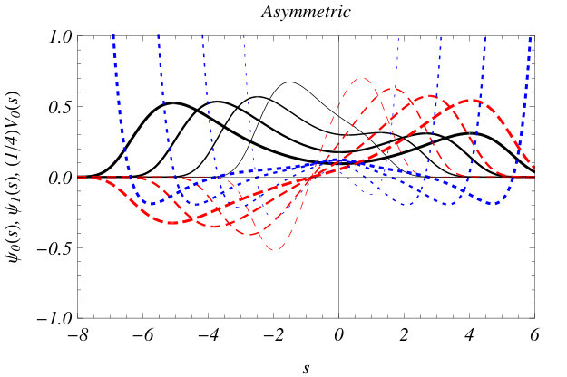 Figure 1
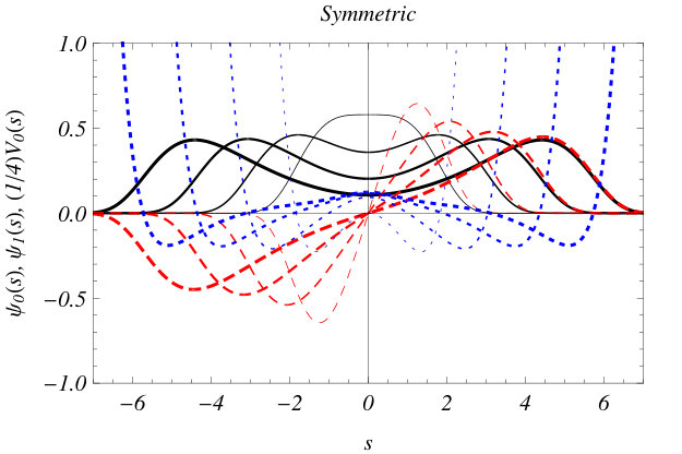 Figure 2
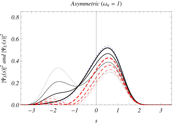 Figure 3
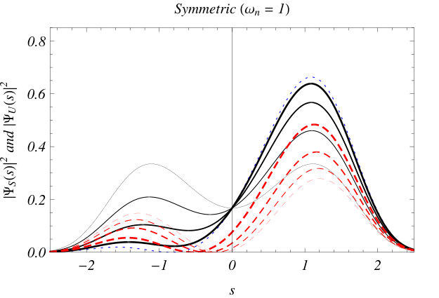 Figure 4
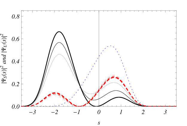 Figure 5
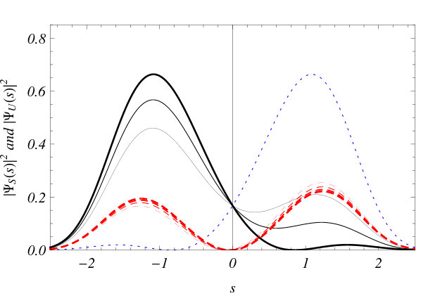 Figure 6
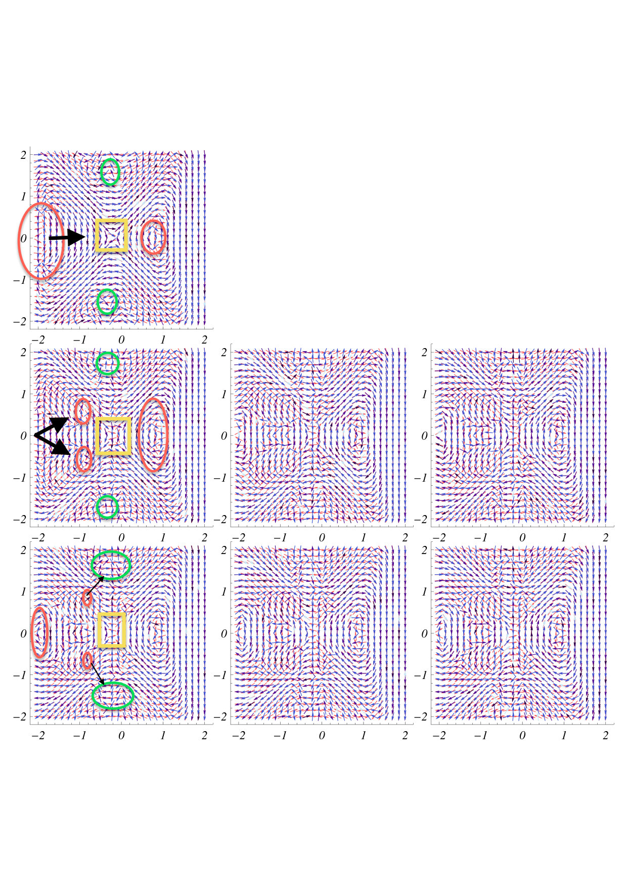 Figure 7
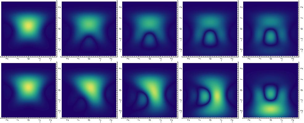 Figure 8
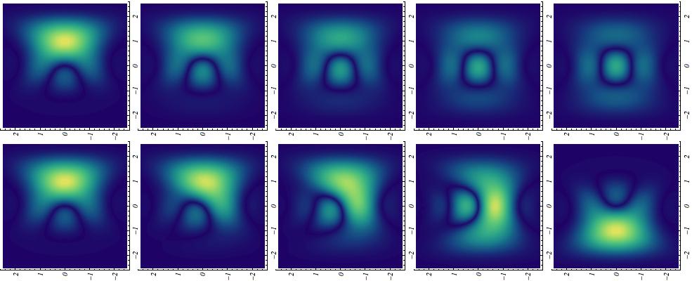 Figure 9
Peer Reviews
No public reviews on file for this paper yet. If you reviewed it on a platform where reviews are public (OpenReview, ICLR, NeurIPS, ICML), you can paste yours below so the community can read it here.
Videos
No videos yet. Explain this paper in a talk, walkthrough, or lecture? Add one.
Topological view of quantum tunneling coherent destruction
Alex E. Bernardini and Mariana Chinaglia
Departamento de Física, Universidade Federal de São Carlos, PO Box 676, 13565-905, São Carlos, SP, Brasil. [email protected]
Abstract
Quantum tunneling of the ground and first excited states in a quantum superposition driven by a novel analytical configuration of a double-well (DW) potential is investigated. Symmetric and asymmetric potentials are considered as to support quantum mechanical zero mode and first excited state analytical solutions. Reporting about a symmetry breaking that supports the quantum conversion of a zero-mode stable vacuum into an unstable tachyonic quantum state, two inequivalent topological scenarios are supposed to drive stable tunneling and coherent tunneling destruction respectively. A complete prospect of the Wigner function dynamics, vector field fluxes and the time dependence of stagnation points is obtained for the analytical potentials that support stable and tachyonic modes.
1 Introduction
The phase-space Wigner-Weyl formalism provides a suitable description of quantum mechanics. In the context of the dynamical evolution of quantum states, the Wigner function helps one to identify highlighting non-classical features revealed, for instance, by quantum tunneling [1, 3, 2]. The investigation of single-particle tunneling in double-well (DW) potentials can be found in several relevant scenarios [4, 5, 6, 7, 8, 9, 10]. For DW potentials, the maximum point () between the two minima plays the role of a barrier that drives the quantum tunneling exhibited by the quantum superposition of ground and first excited states, when their energy are smaller than that from the hump. The quantum tunneling for a function generated by a two-wave superposition supported by novel symmetric and asymmetric DW potential configurations, when described in the phase-space, is investigated in this letter. In particular the dynamics of tachyonic modes supported by modified topological scenarios [11, 12], different from those which holds stable tunneling, is discussed. A symmetry breaking that supports the quantum conversion of a zero-mode stable vacuum into an unstable tachyonic quantum state is assumed [2] as to identify two inequivalent topological scenarios which drive stable tunneling and coherent tunneling destruction, respectively. In this scenarios, the Wigner flow stagnation points can be found where the potential is force free. They depend deeply on the potential critical points and bring on different effects whether they are a minimum, maximum or saddle points identified by winding numbers defined through [1] , where is the angle between the positive position axis and the Wigner flow vectors. After a complete discussion of the tunneling phenomenon where the Wigner functions and their flow vector fields are computed, one identifies the non-classical features regarding the behavior of the stagnation points.
To summarize, proceeding is organized as following: in Sec. , the framework for the calculation of the ground and first excited states for DW potential configurations is presented, and results for a kink-like deforming function [11, 13, 12] are obtained; in Sec. the quantum tunneling and Wigner flow for quantum superposition involving zero-mode stable and tachyonic states are calculated and discussed for symmetric and asymmetric DW configurations; the conclusions are drawn in Sec. .
2 Ground and first excited states in a DW potential
Given the ground state, , of a potential, well-stablished quantum mechanical results, as those from [3], allow one to calculate the corresponding first excited, , state through a multiplier function that relates with as [1]
[TABLE]
Through the substitution of by into the Schrödinger equation for and subtracting the result from the Schrödinger equation for multiplied by , one can find the quantity ,
[TABLE]
where is the energy difference between the states and henceforth shall be conveniently denoted by . Considering that is an ansatz multiplier function, for a ground state described by,
[TABLE]
where is a normalization constant, the first excited state can be calculated through Eq. (1). Once a solution is found, the potential can be straightforwardly calculated through
[TABLE]
An ansatz multiplier function set as [1, 2] which is, up to an additive constant, the solution for the differential equation driven by the model. This multiplier function is an input for both set of potentials: symmetric () and asymmetric () ones. Once one has chosen , it is possible to find through Eq. (2) and proceed with the calculations for and by means of Eq. (3) and Eq. (1), respectively. The potential can be calculated either by means of or through the Eq. (4).
Once and have been established, two inequivalent topological scenarios that supports the quantum conversion of a zero-mode stable vacuum into an unstable tachyonic quantum state can be found. As to see the connection between their energies, one assumes a scalar field equation of motion, derived from a time independent Lagrangian in , from which, through quantum perturbations, by an increment of , it is possible to find the Schrödinger-like equation,
[TABLE]
with , i. e. the quantum mechanical potential analogue. The eigenenergy, when real, i.e. for , leads to a quantum stable solution. When it is imaginary, i.e. for , one deals with unstable functions: the tachyonic modes.
By identifying , with , it is straightforward to show that Eq. (5) can be written as,
[TABLE]
Note that if the energy, , is converted to zero, one has a novel scenario where the Schrödinger-like equation is
[TABLE]
with the novel quantum potential [2]. Now, there is a state that cross the origin producing a node. Eq. (1) thus implies that,
[TABLE]
Once one has the zero mode calculated through Eq. (3) and the potential found in Eq. (4), it is possible to compare it with and identify that . So there is an identification with the corresponding topological scenario that supports quantum perturbations for this potential [2]. In fact, the zero-mode stable vacuum () can work as a mathematical tool for obtaining an unstable quantum state, which behaves like a tachyonic mode. Therefore, in this case, becomes the novel zero-mode stable solution in the tachyonic system causing the appearance of instabilities, as is converted into , namely, an unstable configuration. For a DW potential as in (4) built from the ground state wave function, one identifies
[TABLE]
as well as the multiplier function, , where drives the asymmetric profiles, as obtained from Eq. (4).
The corresponding first excited states are obtained from Eq. (1), also for symmetric and asymmetric DW configurations. Fig. 1 shows the ground and first excited states along with both potentials, symmetric and asymmetric ones.
3 Quantum tunneling and Wigner flow analysis
In order to investigate the quantum tunneling one needs the superposition function of the ground, , and first excited, , states:
[TABLE]
which will be set into the Wigner function:
[TABLE]
where denotes the weight of and in the superposition function. As a quasi-probability function, the Wigner function attains only real values they can also be negative. The modulus of the normalized stable-unitary (black lines), and unstablestationary (red lines) density probabilities are depicted in Fig. 2 for different times, ranging from to (first row) and from to (second row).
It is evidenced through the images that the normalized function completes the tunneling cycle going from right to left for both potentials while the tachyonic cycle is converted into a stationary state after the coherent destruction of the unstable mode. The Wigner functions squared for both scenarios relative to symmetric and asymmetric potentials can be seen in Fig. 3. Analyzing the image it is clear, as was previously seen with Fig. 2, that the tunneling occurs for both functions. The difference appears when one recognizes that for the normalized wave function the tunneling process is invertible whereas for tachyonic functions a limit state is reached. The invertible behavior appears because of the small difference between the energy of the states that causes a beat period, . The complete beating, that is when the function goes from one well to another and returns, is not presented in the tachyonic case because it is not normalizable. This latter smoothly attains an equilibrium lying in equal proportions in the two wells.
The next step corresponds to the calculation of the Wigner flow,
[TABLE]
which, in the classical limit, i.e. when one has or powers , leads to an equivalence between Wigner and classical Liouville flow.
By convenience, the Wigner flow vector fields relative to the stable wave functions driven by the asymmetric potential is considered in Fig. 4 for different times along the tunneling evolution. The first feature that is highlighted through the vector field is the difference between the classical (red) and quantum (blue) vector directions. The larger this difference, the greater the degree of non-classicality of the system [1]. While passing through a minimum of the potential, the flow spins towards this point and one has the winding number . Passing through a maximum of the potential, the flow also spins generating , but it spreads instead of concentrating. If it is a saddle point it elongates the flow making it slower and slower near the central point, through which one has .
Another feature is the flux reversion that corresponds to the regions where the Wigner function attains negative values. In order to investigate this feature ally with the stagnation points position, one can imagine a top-down vertical line around in the first frame of Fig. 4. Following this line it is possible to first recognize one counterclockwise (CCW) vortex (green circle), then a flow reversal followed by a saddle point (yellow square), around . Moving to negative values of one has a CCW vortex, causing again the flow inversion. This behavior is a further indication of the non-classical character of the system.
In order to see the stagnation points dynamics and calculate , the integration loop is depicted in each frame of Fig. 4. Note that the initial total winding number (first frame) is , correspondent to one clockwise (CW) vortex (red circle; ), two CCW vortices (green circles; ) and one saddle point (yellow square); ). In the next frame the saddle point starts to crumble while another CW vortex appears in the left. Besides, one can no longer recognize the CCW vortices, which results again in a total winding number . Considering all subsequent frames one sees that the saddle point completely disappears engendering sequentially . Consequently, charge conservation is attained as conjectured [1]. The novelty is that an opposite conclusion appears when considering the unstable case for which one has no charge conservation. For the unstable function however this lack of conservation is not totally a surprise, once it is predicted only for systems with unitary quantum dynamics. Finally, the stagnation points also work as a tool for the recognition of tunneling. The function , which is found initially only in the right minimum of the potential, appears in the form of a CW vortex near in Fig. 4. After time evolution coexists in both minima, thus causing the appearance of another CW vortex in the left-side in some subsequent frames. This behavior reveals the tunneling through the stagnation points.
4 Conclusions
Quantum tunneling analysis has shown that one has a reversibility of the process for the stable wave function whereas the tachyonic function attains a limit coexisting in both wells for any subsequent time. Thereat one can say that the tunneling undergoes a process of coherent destruction. It was also noticed that the Wigner vector field can be used to study non-classical features since it evinces the differences between quantum and classical vector flux profiles as well as the flow reversibility. The latter occurs where one has negative values for the Wigner function related to the stagnation points. Lastly, while one finds the expected charge conservation for stable wave functions, one draws attention to the fact that this conservation is not in principle expected for unstable functions. In fact, it is depicted from the vector flow analysis for the tachyonic case.
\ack
AEB thanks for the financial support from the Brazilian Agency FAPESP (grant 15/05903-4).
References
- [1]
Steuernagel O, Kakofengitis D and Ritter G 2013 Phys. Rev. Lett. 110 030401
- [2]
Bernardini A E and Chinaglia M 2015 Mod. Phys. Lett. A30 1550118
- [3]
Caticha A 1995 Phys. Rev. A 51 4264
- [4]
Domcke W, Hänggi P and Tannor D 1997 Chem. Phys. 217 117
- [5]
Schulz M D, Dusuel S, Schmidt K P and Vidal J 2013 Phys. Rev. Lett. 110 147203
- [6]
Casetti L, Cohen E G D and Pettini M 1999 Phys. Rev. Lett. 82 4160
- [7]
Bernardini A E and Bertolami O 2013 Phys. Lett. B726 512
- [8]
Bernardini A E and da Rocha R 2012 Phys. Lett. B717 238
- [9]
Bernardini A E and da Rocha R 2013 AHEP 2013 304980
- [10]
Bernardini A E, Chinaglia M and da Rocha 2015 Eur. Phys. J Plus 130 97
- [11]
Bernardini A E and da Rocha R 2016 Phys. Lett. A380 2279
- [12]
Bernardini A E, Chinaglia M and da Rocha R 2016 Int. J. Theor. Phys. 55 4605
- [13]
Bernardini A E and da Rocha R 2016 AHEP 2016 3650632
The reference list from the paper itself. Each links out to its DOI / PubMed record.
- 1[1] Steuernagel O, Kakofengitis D and Ritter G 2013 Phys. Rev. Lett. 110 030401
- 2[2] Bernardini A E and Chinaglia M 2015 Mod. Phys. Lett. A 30 1550118
- 3[3] Caticha A 1995 Phys. Rev. A 51 4264
- 4[4] Domcke W, Hänggi P and Tannor D 1997 Chem. Phys. 217 117
- 5[5] Schulz M D, Dusuel S, Schmidt K P and Vidal J 2013 Phys. Rev. Lett. 110 147203
- 6[6] Casetti L, Cohen E G D and Pettini M 1999 Phys. Rev. Lett. 82 4160
- 7[7] Bernardini A E and Bertolami O 2013 Phys. Lett. B 726 512
- 8[8] Bernardini A E and da Rocha R 2012 Phys. Lett. B 717 238