On the Dynamics of Deterministic Epidemic Propagation over Networks
Wenjun Mei, Shadi Mohagheghi, Sandro Zampieri, Francesco Bullo

TL;DR
This paper reviews deterministic nonlinear models for infectious disease spread over contact networks, analyzing equilibria, stability, and thresholds for SI, SIS, and SIR models, with new results on endemic states and transient behavior.
Contribution
It provides novel analytical results and algorithms for the stability, endemic states, and transient dynamics of network-based epidemic models.
Findings
Established equilibria and stability for SI model
Characterized endemic states and thresholds for SIS model
Proposed an iterative algorithm for SIR asymptotic states
Abstract
In this work we review a class of deterministic nonlinear models for the propagation of infectious diseases over contact networks with strongly-connected topologies. We consider network models for susceptible-infected (SI), susceptible-infected-susceptible (SIS), and susceptible-infected-recovered (SIR) settings. In each setting, we provide a comprehensive nonlinear analysis of equilibria, stability properties, convergence, monotonicity, positivity, and threshold conditions. For the network SI setting, specific contributions include establishing its equilibria, stability, and positivity properties. For the network SIS setting, we review a well-known deterministic model, provide novel results on the computation and characterization of the endemic state (when the system is above the epidemic threshold), and present alternative proofs for some of its properties. Finally, for the network…
Click any figure to enlarge with its caption.
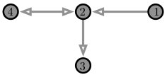 Figure 1
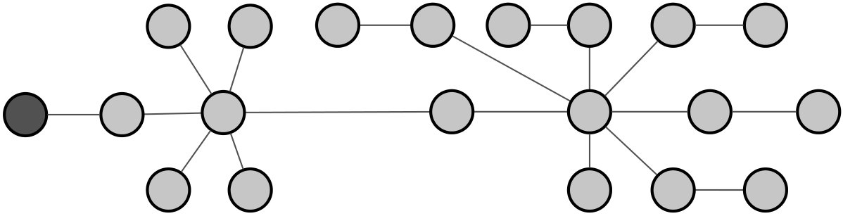 Figure 2
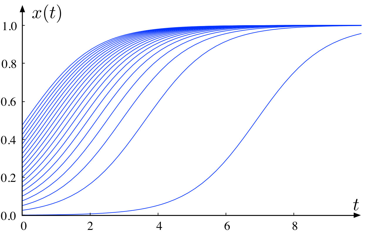 Figure 3
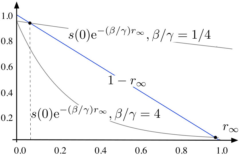 Figure 4
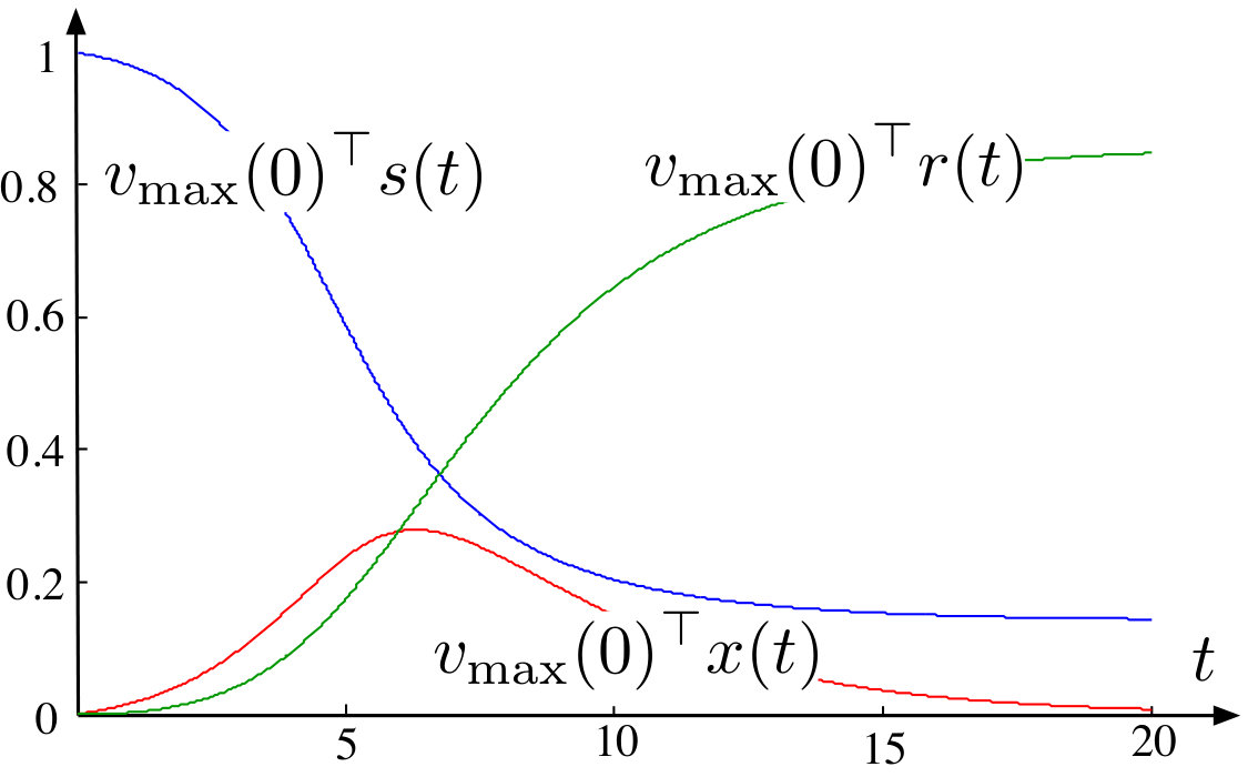 Figure 5
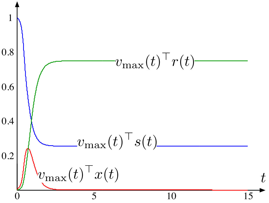 Figure 6
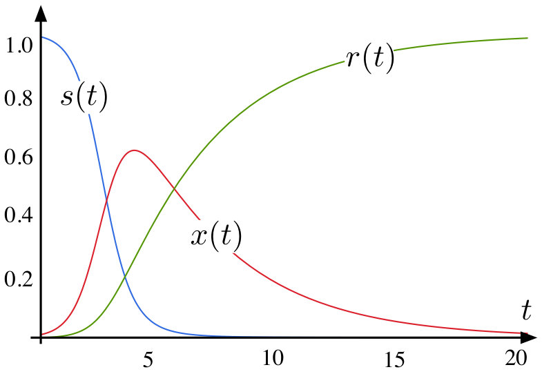 Figure 7
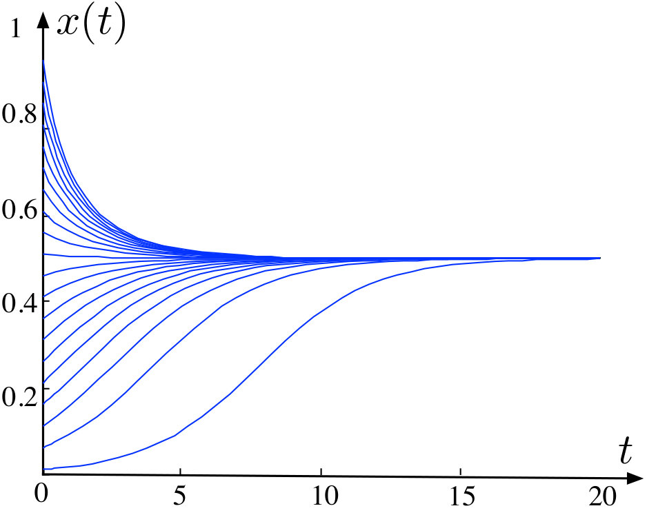 Figure 8
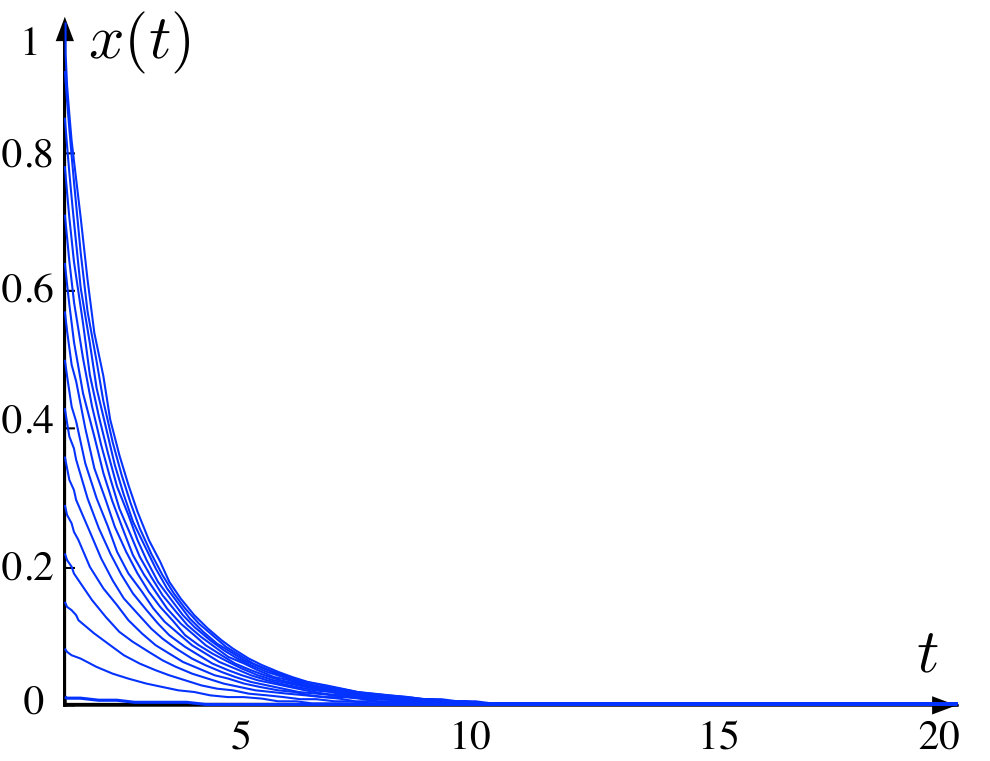 Figure 9
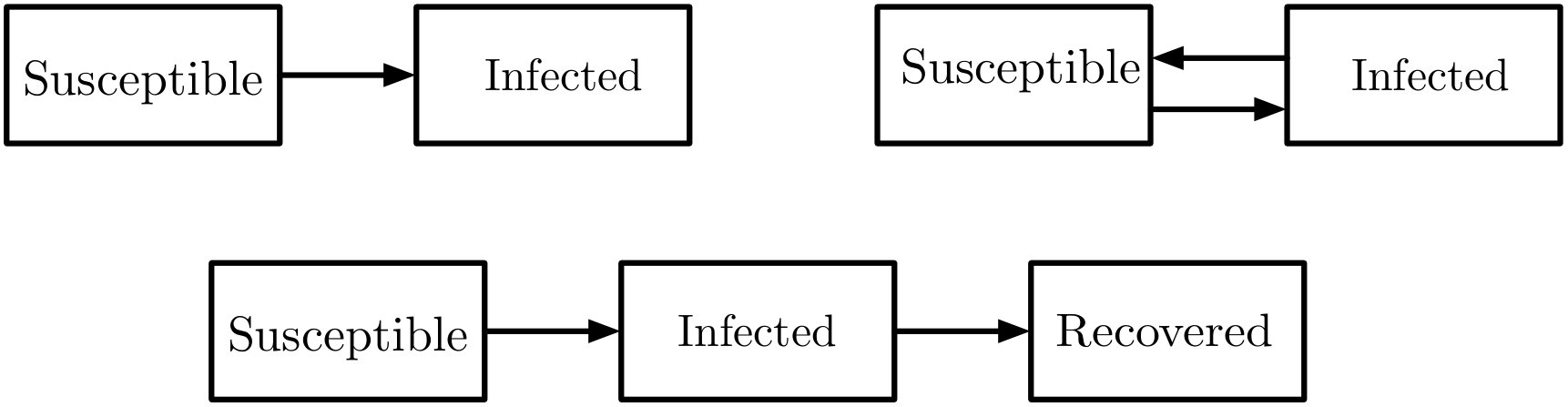 Figure 10
 Figure 11
 Figure 12
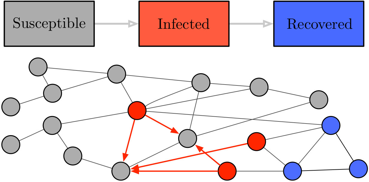 Figure 13
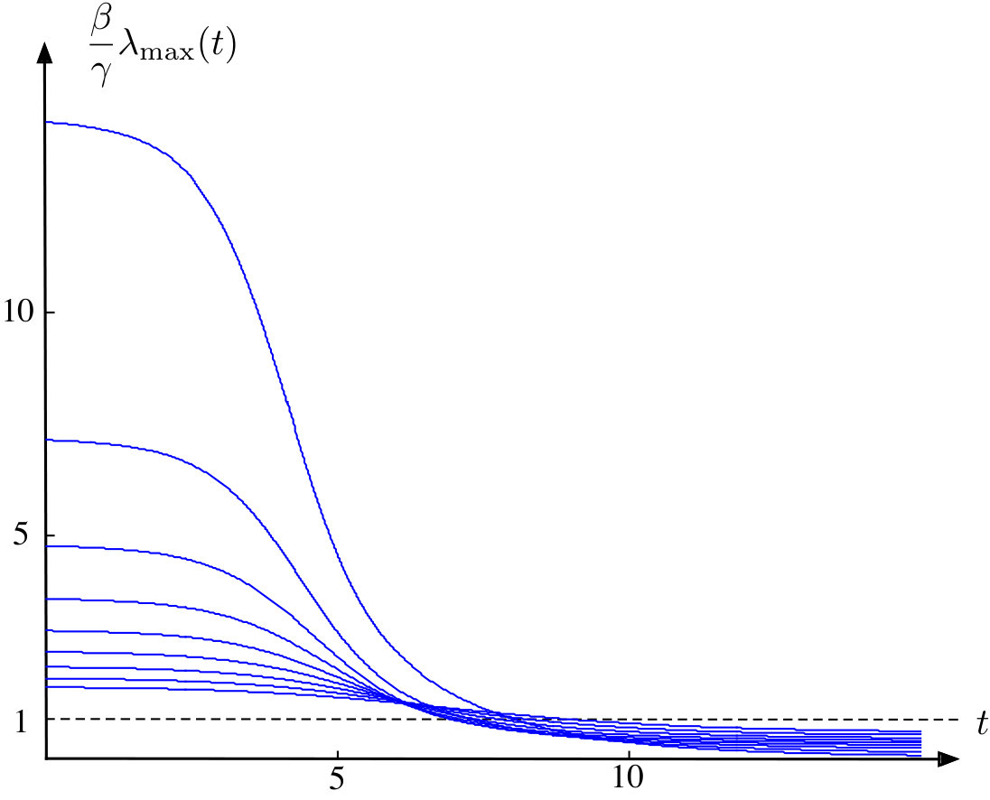 Figure 14
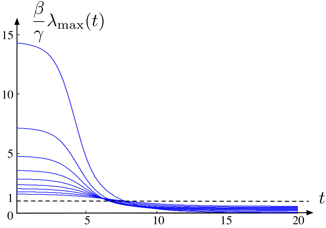 Figure 15
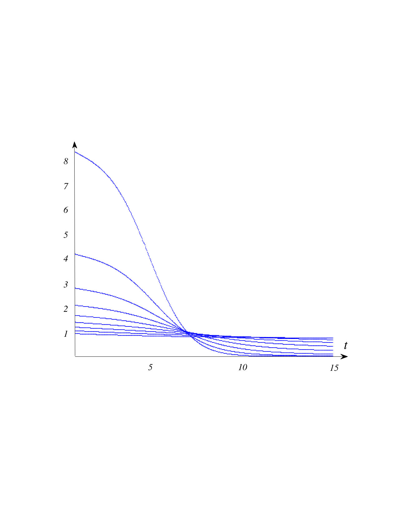 Figure 16
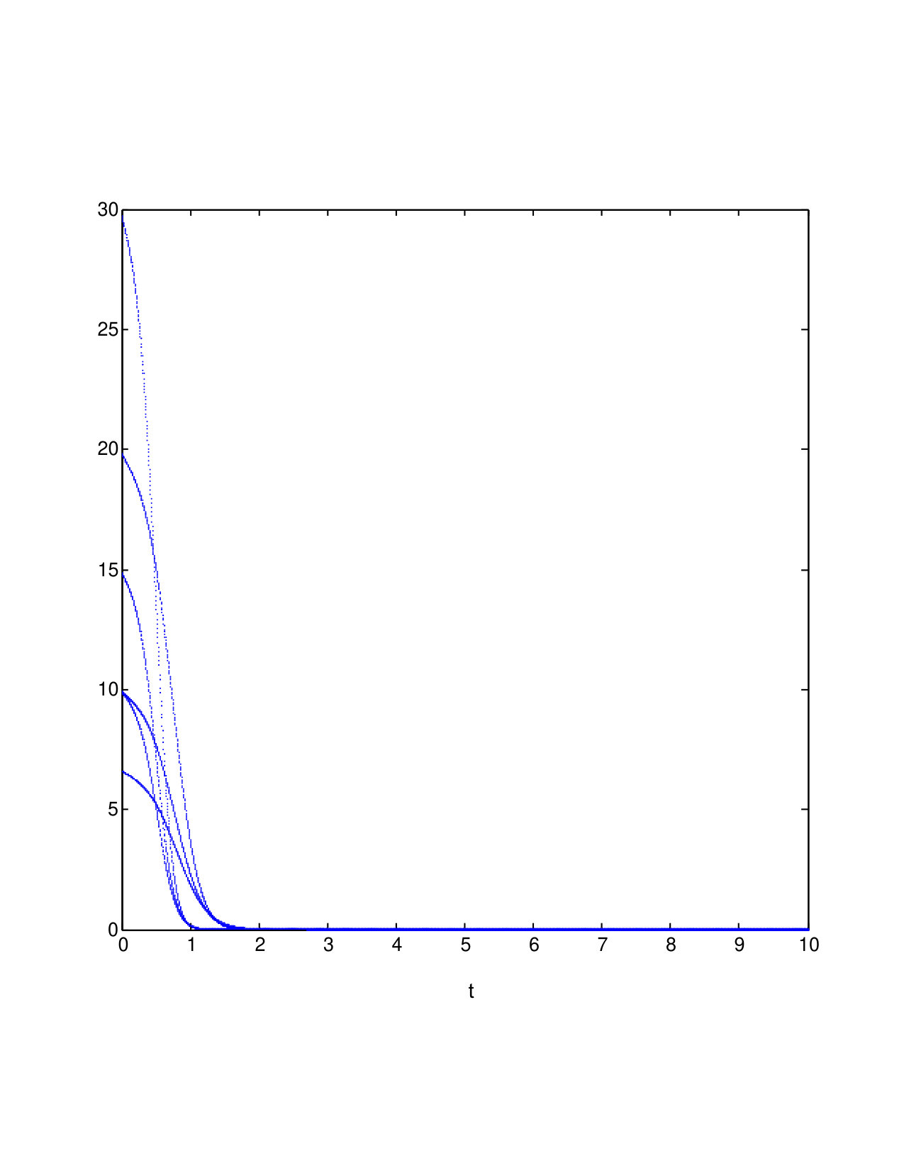 Figure 17
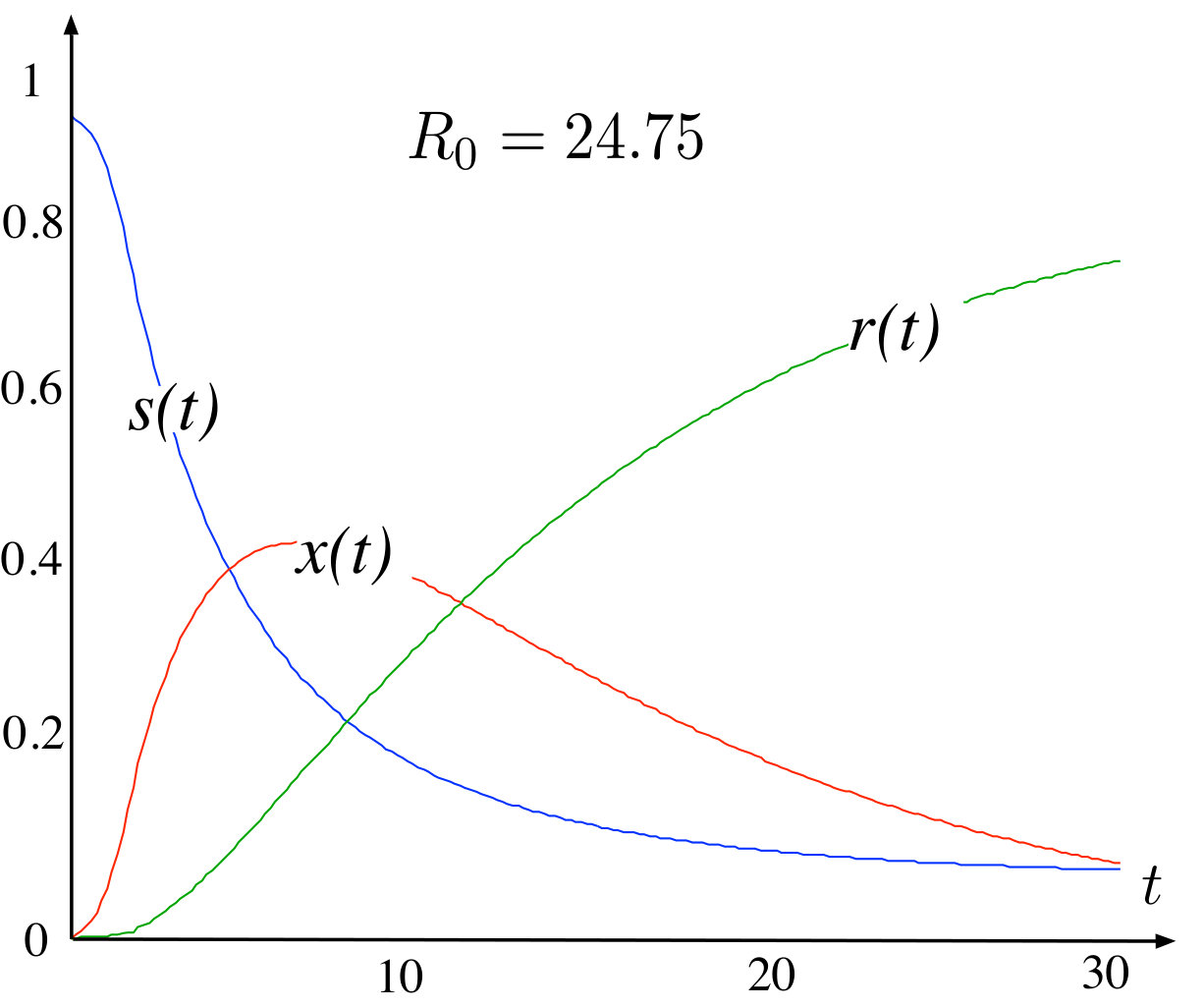 Figure 18
 Figure 19
 Figure 20
 Figure 21
 Figure 22
 Figure 23
Peer Reviews
No public reviews on file for this paper yet. If you reviewed it on a platform where reviews are public (OpenReview, ICLR, NeurIPS, ICML), you can paste yours below so the community can read it here.
Videos
No videos yet. Explain this paper in a talk, walkthrough, or lecture? Add one.
Taxonomy
TopicsMathematical and Theoretical Epidemiology and Ecology Models · Complex Network Analysis Techniques · Opinion Dynamics and Social Influence
On the Dynamics of Deterministic Epidemic Propagation over Networks††thanks: This material is based upon work supported by, or
in part by, the U. S. Army Research Laboratory and the U. S. Army Research Office under grant numbers W911NF-15-1-0577.
Wenjun Mei Shadi Mohagheghi Sandro Zampieri Francesco Bullo Wenjun Mei and Francesco Bullo are with the Department of Mechanical Engineering and with Center for Control, Dynamical Systems, and Computation, University of California, Santa Barbara, Santa Barbara, CA 93106, USA, [email protected], [email protected] Shadi Mohagheghi is with the Department of Electrical and Computer Engineering, University of California at Santa Barbara, Santa Barbara, CA 93106, USA, [email protected] Sandro Zampieri is with the Department of Information Engineering, University of Padova, Italy, [email protected]
Abstract
In this work we review a class of deterministic nonlinear models for the propagation of infectious diseases over contact networks with strongly-connected topologies. We consider network models for susceptible-infected (SI), susceptible-infected-susceptible (SIS), and susceptible-infected-recovered (SIR) settings. In each setting, we provide a comprehensive nonlinear analysis of equilibria, stability properties, convergence, monotonicity, positivity, and threshold conditions. For the network SI setting, specific contributions include establishing its equilibria, stability, and positivity properties. For the network SIS setting, we review a well-known deterministic model, provide novel results on the computation and characterization of the endemic state (when the system is above the epidemic threshold), and present alternative proofs for some of its properties. Finally, for the network SIR setting, we propose novel results for transient behavior, threshold conditions, stability properties, and asymptotic convergence. These results are analogous to those well-known for the scalar case. In addition, we provide a novel iterative algorithm to compute the asymptotic state of the network SIR system.
Index terms: network propagation model, nonlinear dynamical system, phase transition, mathematical epidemiology
1 Introduction
1.1 Motivation and problem description
Propagation phenomena appear in numerous disciplines. Examples include the spread of infectious diseases in contact networks, the transmission of information in communication networks, the diffusion of innovations in competitive economic networks, cascading failures in power grids, and the spreading of wild-fires in forests. Scalar models of propagation phenomena have been widely studied, e.g., see the survey by Hethcote [12] on scalar epidemic spreading models. These models qualitatively capture some dynamic features, including phase transitions and asymptotic states. However, shortcomings of these scalar models are also prominent: for example, scalar models are typically based on the assumption that individuals in the population have the same chances of interacting with each other. This assumption overlooks the internal structure of the network over which the propagation occurs, as well as the heterogeneity of individuals in the network. Both these aspects play critical roles in shaping the sophisticated dynamical behavior of the propagation processes.
In a general formulation, propagation is a stochastic process on a complex network. Its features are determined by the properties of local node-to-node exchanges as well as of the global contact networks. Stochastic propagation processes can be modeled as Markov chains of exponential dimensions in the size of the network. Due to these properties of propagation processes, many relevant research questions arise naturally. Three key questions are: (1) how to deal with the lack of well-quantified local details of the complex networks; (2) how to identify the models and parameters, and estimate the states of such stochastic large-dimension phenomena, and (3) how to analyze the transient and asymptotic properties of their dynamics.
Three approaches are commonly adopted in the analysis of propagation models. The first is to directly characterize the stochastic process adopting tools from branching processes, percolation, and random graph theory; e.g., see [7]. The second approach proposes a degree-based model based on the approximation that nodes with the same degree exhibit similar behavior; e.g., see [17, Chapter 17]. The first two approaches are both based on the random graphs for which global characteristics can be estimated statistically, such as the degree distribution. The third approach is based on the mean-field approximation of Markov-chain models and algebraic graph theory; this approach results in a deterministic network model. Distinct from the first two approaches, the mean-field models first assume knowledge of the local propagation parameters and then relate the dynamical behavior of the propagation process to some global parameters of the network, which can be estimated without knowing the full local details, e.g., the spectral radius of the network’s adjacency matrix. One of the main advantages of the mean-field approach is that, by representing the network as an adjacency matrix, well-established theorems in matrix analysis and dynamical systems can be applied to the analysis of some sophisticated behavior of the propagation processes.
In this paper we review a class of epidemic propagation models which adopt the third approach. Distinct in the assumptions on the microscopic features of the disease and the individual behavior, the epidemic propagation models we focus on are classified into three types: the Susceptible-Infected (SI) model, the Susceptible-Infected-Susceptible (SIS) model and the Susceptible-Infected-Recovered (SIR) model; basic representations of these models are illustrated in Figure 1. In this work we review models of these three types over networks and characterize their dynamical properties. In short, we study the network SI, network SIS, and network SIR models.
1.2 Literature review
The dynamics of several classic scalar epidemic models, i.e., the population models without network structure, are surveyed in detail by Hethcote [12]. Among the different metrics discussed, identifying the effective reproduction number is of particular interest to researchers; is the expected number of individuals that a randomly infected individual can infect during its infection period. In these scalar models, whether an epidemic outbreak occurs or the disease dies down depends upon whether or , i.e., upon whether the system is above or below the so-called epidemic threshold. Here by epidemic outbreak we mean an exponential growth of the fraction of the infected population for small time. The basic reproduction number is the effective reproduction number in a fully-healthy susceptible population. In what follows we focus our review on deterministic network models.
The earliest work on the (continuous-time heterogeneous) SIS model on networks is [14]. This work proposes an -dimensional model on a contact network and analyzes the system’s asymptotic behavior. This article proposes a rigorous analysis of the threshold for the epidemic outbreak, which depends on both the disease parameters and the spectral radius of the contact network. For the case when the basic reproduction number is above the epidemic threshold, this paper establishes the existence and uniqueness of a nonzero steady-state infection probability, called the endemic state. In what follows we refer to the model proposed by Lajmanovich et al. [14] as the network SIS model; it is also known as the multi-group or multi-population SIS model. Numerous extensions and variations on these basic results have appeared over the years.
Allen [2] proposes and analyzes a discrete-time network SIS model. This work appears to be the first to revisit and formally reproduce, for the discrete-time case, the earlier results by Lajmanovich et al. [14]; see also the later work by Wang et al. [21]. This work confirms the existence of an epidemic threshold, as a function of the spectral radius of the contact network. Further recent results on the discrete-time model are obtained by Ahn et al. [1] and by Azizan Ruhi et al. [3].
Van Mieghem et al.[20] argue that the (continuous-time) network SIS model is in fact the mean-field approximation of the original Markov-chain SIS model of exponential dimension; this claim is rigorously proven by Sahneh et al. [19]. Van Mieghem et al. [20] refer to this model as the intertwined SIS model and write the endemic state as a continued fraction.
The works by Fall et al. [9] and Khanafer et al. [13] discuss the continuous-time network SIS model in a more modern language. Fall et al. [9] refer to this model as the -group SIS model and apply Lyapunov techniques and Metzler matrix theory to establish existence, uniqueness, and stability of the equilibrium points below and above the epidemic threshold. Khanafer et al. [13] use positive system theory in their analysis and extend the existence, uniqueness, and stability results to the setting of weakly connected digraphs.
An early work by Hethcote [11] proposes a general multi-group SIR model with birth, death, immunization, and de-immunization. The epidemic threshold and the equilibria below/above the threshold are characterized. For the simplified model without birth/death and de-immunization, Hethcote [11] proves that the system converges asymptotically to an all-healthy state. Guo et al. [10] consider a generalized network SIR model with vital dynamics, that is, with birth and death. They characterize the basic reproduction number and, through a careful Lyapunov analysis, show the existence and global asymptotic stability of an endemic state above the threshold. Youssef et al. [22] study a special case of the network SIR model under the name of individual-based SIR model over undirected networks. Through a simulation-based analysis, the epidemic threshold is given as a function of the spectral radius of the network. To the best of our knowledge, no works have comprehensively characterized the properties of the network SI model.
We conclude by mentioning other surveys and textbook treatments. In [15], the stability of equilibria for the SEIR model is reviewed through Lyapunov and graph theory. The additional state represents the exposed population, i.e., the individuals who are infected but not infectious. The book chapters [17, Chapter 17], [8, Chapter 21], and [4, Chapter 9] review various heterogeneous epidemic models. The recent survey by Nowzari et al. [18] presents various epidemic models and addresses many solved and open problems in the control of epidemic spreading.
1.3 Statement of Contribution
The contributions of this work are as follows: in each section, we start by reviewing the scalar SI, SIS, and SIR models; these are the models in which variables represent an entire “well-mixed” population or nodes of an all-to-all unweighted graph. We then focus our discussion on multi-group network models and provide a tutorial comprehensive treatment with comprehensive statements and proofs for the network SI, SIS and SIR models.
We first introduce and analyze the novel network SI model. We analyze its asymptotic convergence, positivity of infection probabilities, initial growth rate, and the stability of equilibria. We show that in the network SI model, the system does not display a threshold and all the trajectories converge to the full contagion state.
Next we focus on the network SIS model. We review some results in [14, 9, 13] regarding the dynamical behavior of the system below and above the threshold, and present alternative proofs for them. For systems above the epidemic threshold, we present a novel provably-correct iterative algorithm for computing the fraction of infected individuals converging to the endemic state. We present novel Taylor expansions for the endemic state near the epidemic threshold and in the limit of high infection rates. Finally, we show that the spread of infection takes place instantaneously upon infecting at least one node in the network.
Finally, for the network SIR model, we present novel transient behavior and system properties. We propose new threshold conditions above which the epidemic grows initially, and below which it exponentially dies down. We show that, along all system trajectories, the infected population asymptotically vanishes and the epidemic asymptotically dies down. The initial rate of growth above the threshold is given in terms of network characteristics, initial conditions, and infection parameters. We show that our proposed weighted average of the infected population, obtained by the entries of dominant eigenvector of an irreducible quasi-positive matrix, captures information regarding the distribution of infection in the system. We also establish positivity of the infection probabilities and certain monotonicity properties. Moreover, we provide a novel iterative algorithm to compute the asymptotic state of the network SIR model, with any arbitrary initial condition. For the iterative algorithm, the existence and uniqueness of the fixed point, and the convergence of the iteration are rigorously proved. Our results are analogous to the scalar SIR model properties and are valid for any arbitrary network topologies. In comparison with [22], our treatment builds on their numerical results but our result is more general in that it does not depend upon specific initial conditions and graph topologies, and establishes numerous properties, including the novel characterization of epidemic threshold.
Finally, we remark that our deterministic network models are derived from the Markov-chain models through a mean-field approximation. We do not discuss here the Markov-chain model and the approximation process and refer instead to [19] and [6, Chapter 17].
1.4 Organization
Section 2 introduces our model set-up and some preliminary notations. The SI, SIS and SIR models are presented, respectively, in Sections 3, 4, and 5. Section 6 is the conclusion.
2 Model Set-Up and Notations
For the scalar models, we use the notation ( and resp.) for the fraction of infected (susceptible and recovered resp.) individuals in the population at time . The rest of this section is about the notations and basic model set-up for the network epidemic model.
a) Contact Network: The epidemics are assumed to propagate over a weighted digraph , where and is the set of directed links. Nodes of can be interpreted as either single individuals in the contact network or as homogeneous populations of individuals at each location/node in the contact network. denotes the adjacency matrix associated with . For any , , characterizes the contact strength from node to node . For , and for , . In this paper, is assumed to be strongly connected.
b) Node States and Probabilities: For different epidemic propagation models, the set of possible node states are distinct. For network SI or SIS models, each node can be in either the “susceptible” or “infected” state, while in the network SIR model, there is an additional possible node state: “recovered.” For a graph in which the nodes are single individuals, let ( and resp.) be the probability that individual is in the susceptible (infected and recovered resp.) state at time . Alternatively, if the nodes are considered to be the populations, then ( and resp.) is interpreted as the fraction of susceptible (infected and recovered resp.) individuals in population . In this paper, without loss of generality, we adopt the interpretation of nodes as single individuals.
c) Frequently Used Notations: The symbol denotes the set of real numbers, while denotes the set of non-negative real numbers. The symbol denotes the empty set. For any two vectors , we write
[TABLE]
We adopt the shorthand notations and . Given , let denote the diagonal matrix whose diagonal entries are . For an irreducible nonnegative matrix , let denote the dominant eigenvalue of that is equal to the spectral radius . Moreover, we let ( resp.) denote the corresponding entry-wise strictly positive left (right resp.) eigenvector associated with , normalized to satisfy (resp. ). The Perron-Frobenius Theorem for irreducible matrices guarantees that , and are well defined and unique. Where not ambiguous, we will drop the argument and, for example, write
[TABLE]
with and ; and .
3 Susceptible-Infected Model
In this section, we first review the classic scalar susceptible-infected (SI) model, and then present and characterize the network SI model.
3.1 Scalar SI model
The scalar SI model assumes that the growth rate of the fraction of the infected individuals is proportional to the fraction of the susceptible individuals, multiplied by a so-called infection rate . The model is given by
[TABLE]
and its dynamical behavior is given by the lemma below.
Lemma 1** (Dynamical behavior of the SI model).**
Consider the scalar SI model (1) with . The solution from initial condition is
[TABLE]
All initial conditions result in the solution being monotonically increasing and converging to the unique equilibrium as .
Solutions to equation (1) with different initial conditions are plotted in Figure 2. The SI model (1) results in an evolution akin to a logistic curve, and is also called the logistic equation for population growth.
3.2 Network SI model
The network SI model on a weighted digraph with the adjacency matrix is given by
[TABLE]
or, in equivalent vector form,
[TABLE]
where is the infection rate. Alternatively, in terms of the fractions of susceptibile individuals , the network SI model is
[TABLE]
The following results and their proof are novel.
Theorem 2** (Dynamical behavior of network SI model).**
Consider the network SI model (4) with . For strongly connected graph with adjacency matrix , the following statements hold:
- (i.
if , then for all . Moreover, is monotonically non-decreasing (here by monotonically non-decreasing we mean for all ). Finally, if , then for all ; 2. (ii.
the model (4) has two equilibrium points: (no epidemic), and (full contagion);
- (a)
the linearization of model (4) about the equilibrium point is and it is exponentially unstable; 2. (b)
let be the degree matrix. The linearization of model (5) about the equilibrium is and it is exponentially stable; 3. (iii.
each trajectory with initial condition converges asymptotically to , that is, the epidemic spreads monotonically to the entire network.
Proof.
(i) The fact that, if , then for all means that is an invariant set for the differential equation (4). This is the consequence of Nagumo’s Theorem (see Theorem 4.7 in [5]), since for any belonging on the boundary of the set , the vector \beta\Big{(}I_{n}-\operatorname{diag}\!\big{(}x\big{)}\Big{)}Ax is either tangent, or points inside the set .
Observe that the invariance of the set implies that and so for all .
We want to prove now that,if , then for all . If by contradiction there is and such that , then the monotonicity of would imply that for all , which would yield for all . By (3) this would imply that for all for all such that . We could iterate this argument and using the irreducibility of we would get the contradiction that for all concluding in this way the proof of (i.
(ii) Regarding statement (ii, note that and are clearly equilibrium points. Let be an equilibrium and assume that . Then there is such that . Since \beta\big{(}1-\bar{x}_{i}\big{)}\sum_{j=1}^{n}a_{ij}\bar{x}_{j}=0, then which implies that for all such that . By iterating this argument and using the irreducibility of we get that concluding only and are equilibrium points. Statements (iia and (iib are obvious. Exponential stability of the linearization is obvious, and the Perron-Frobenius Theorem implies the existence of the unstable positive eigenvalue for the linearization .
(iii) Consider the function ; this is a smooth function defined over the compact and forward invariant set (see statement (i). Since \dot{V}=-\beta\mathbbold{1}_{n}^{\top}\big{(}I_{n}-\operatorname{diag}(x)\big{)}Ax, we know that for all and if and only if . The LaSalle Invariance Principle implies that all trajectories with converge asymptotically to either or . Additionally, note that for all , that if and only if and that if and only if . Therefore, all trajectories with converge asymptotically to . ∎
For the adjacency matrix , there exists a non-singular matrix such that , where is the Jordan normal form of . Since is non-negative and irreducible, according to Perron-Frobenius theorem, the first Jordan block and for any other eigenvalue of . Consider now the onset of an epidemic in a large population characterized by a small initial infection much smaller than . The system evolution is approximated by . This “initial-times” linear evolution satisfies
[TABLE]
where is the first standard basis vector in and denotes a time-varying vector that vanishes as . Let denote the first column of and let denote the first row of . Since and , one can check that ( resp.) is the right (left resp.) eigenvector of associated with the eigenvalue . Since , we have . therefore,
[TABLE]
That is, the epidemic initially experiences exponential growth with rate and with distribution among the nodes given by the eigenvector .
Now suppose that at some time , for all we have that , where each is much smaller than . Then, for time , the approximated system for is given by:
[TABLE]
From the discussion above, we conclude that the initial infection rate is proportional to the eigenvector centrality, and the final infection speed is proportional to the degree centrality.
4 Susceptible-Infected-Susceptible model
In this section we review the Susceptible-Infected-Susceptible (SIS) epidemic model. In addition to the existence of an infection process with rate , this model assumes that the infected individuals recover to the susceptible state at so-called recovery rate .
4.1 Scalar SIS model
In the scalar SIS model, the population is divided into two fractions: the infected and the susceptible , with , obeying the following dynamics:
[TABLE]
The dynamical behavior of system (7) is given below.
Lemma 3** (Dynamical behavior of the SIS model).**
For the SIS model (7) with and :
- (i.
the closed-form solution to equation (7) from initial condition , for , is
[TABLE] 2. (ii.
if , all trajectories converge to the unique equilibrium (i.e., the epidemic disappears); 3. (iii.
if , then each trajectory from an initial condition converges to the exponentially stable equilibrium , which is called the endemic state.
Case (iii corresponds to the case in which epidemic outbreaks take place and a steady-state epidemic contagion persists. The basic reproduction number in this deterministic scalar SIS model is given by . Simulations regarding to Lemma 3(ii and (iii are shown in Figure 3.
4.2 Network SIS Model
In this section we study the network SIS model which is closely related to the original “multi-group SIS model” proposed by Lajmanovich [14]; see also the intertwined SIS model in [20].
The network SIS model with infection rate and recovery rate is given by:
[TABLE]
or, in equivalent vector form,
[TABLE]
In the rest of this section we study the dynamical properties of this model. We start by defining the monotonically-increasing functions
[TABLE]
for and . Note that for all . For vector variables and , we write , and .
Behavior of System Below the Threshold
In this subsection, we characterize the behavior of the network SIS model in a regime we describe as “below the threshold.”
Theorem 4** (Dynamical behavior of the network SIS model: Below the threshold).**
Consider the network SIS model (9), with and , over a strongly connected digraph with adjacency matrix . Let and be the dominant eigenvalue of and the corresponding normalized left eigenvector respectively. If , then
- (i.
if , then for all . Moreover, if , then for all ; 2. (ii.
there exists a unique equilibrium point , the linearization of (9) about is and it is exponentially stable; 3. (iii.
from any , the weighted average is monotonically and exponentially decreasing, and all the trajectories converge to .
Historically, it is meaningful to attribute this theorem to [14], even if the language adopted here is more modern.
Proof.
(i As in Theorem 2 the first part is the consequence of Nagumo’s Theorem. Then define . Notice that this variable satisfies the differential equation . From the same arguments used in the proof of the point (i of Theorem 2 we argue that for all . From this it follows that also for all .
(ii Assume that is an equilibrium point. It is easy to se that . Observe moreover that is an equilibrium point if and only if or, equivalently, if and only if F_{+}\big{(}\tfrac{\beta}{\gamma}Ax^{*}\big{)}=x^{*}. This means that is an equilibrium if and only if it is a fixed point of , where \mathcal{F}(x):=F_{+}\big{(}\tfrac{\beta}{\gamma}Ax\big{)}. Let . For , note because . Moreover, implies that . Therefore, if , then , for all . Since is Schur stable, then . This shows that the only fixed point of is zero.
Next, the linearization of equation (10) is verified by dropping the second-order terms. The linearized system is exponentially stable at for because is larger, in real part, than any other eigenvalue of by the Perron-Frobenius Theorem for irreducible matrices.
(iii Finally, regarding statement (iii, define and note that \big{(}I_{n}-\operatorname{diag}(z)\big{)}v_{\max}\leq v_{\max} for any . Therefore,
[TABLE]
By the Grönwall-Bellman Comparison Lemma, is monotonically decreasing and satisfies from all initial conditions . This concludes our proof of statement (iii. ∎
Behavior of System Above the Threshold
We present the dynamical behavior of the network SIS model above the threshold as follows.
Theorem 5** (Dynamical behavior of the network SIS model: Above the threshold).**
Consider the network SIS model (9), with and , over a strongly connected digraph with adjacency matrix . Let be the dominant eigenvalue of and let and be the corresponding normalized left and right eigenvectors respectively. Let . If , then
- (i.
if , then for all . Moreover, if , then for all ; 2. (ii.
* is an equilibrium point, the linearization of system (10) at is unstable due to the unstable eigenvalue (i.e., there will be an epidemic outbreak);* 3. (iii.
besides the equilibrium , there exists a unique equilibrium point , called the endemic state, such that
- (a)
, 2. (b)
* as , where and*
[TABLE] 3. (c)
, at fixed , as , 4. (d)
define a sequence by
[TABLE]
If is a scalar multiple of and satisfies either or , then
[TABLE]
Moreover, if , then is monotonically non-decreasing; if , then is monotonically non-increasing. 4. (iv.
the endemic state is locally exponentially stable and its domain of attraction is .
Note: statement (ii means that, near the onset of an epidemic outbreak, the exponential growth rate is and the outbreak tends to align with the dominant eigenvector ; for more details see the discussion leading up to the approximate evolution (6). The basic reproduction number for this deterministic network SIS model is given by .
Historically, the existence of a unique endemic state and its global attractivity properties are due to [14]. To the best of our knowledge, the Taylor expansions in parts (iiib and (iiic and the algorithm in part (iiid are novel. The proofs of statements (iii based on the properties of the map are novel.
Proof of selected statements in Theorem 5.
(i This point can be proved as done in point (i of Theorem 2.
(ii This follows from the same analysis of the linearized system as in the proof of Theorem 4(ii.
(iii We begin by establishing two properties of the map , for . First, we claim that, implies . Indeed, note that being connected implies that the adjacency matrix has at least one strictly positive entry in each row. Hence, implies and, since is monotonically increasing, implies .
Second, we observe that, for any and , we have if and only if . Suppose is a scalar multiple of and . We have
[TABLE]
Therefore, the sequence defined by equation (11) satisfies , which in turn leads to , and by induction, for any . Such sequence is monotonically non-decreasing and entry-wise upper bounded by . Therefore, as diverges, converges to some such that F_{+}\big{(}\hat{A}x^{*}\big{)}=x^{*}. This proves the existence of an equilibrium as claimed in statements (iiia and (iiid.
Similarly, for any and , if and only if . Following the same line of argument in the previous paragraph, one can check that the defined by equation (11) is monotonically non-increasing and converges to some , if is a scalar multiple of and satisfies .
Now we establish the uniqueness of the equilibrium . First, we claim that an equilibrium point with an entry equal to [math] must be . Indeed, assume is an equilibrium point and assume for some . The equality implies that also any node with must satisfy . Because is connected, all entries of must be zero. Second, by contradiction, we assume there exists another equilibrium point distinct from . Let and let such that . Then and . Notice that we can assume with no loss of generality that otherwise we exchange and . Observe now that
[TABLE]
Therefore, \big{(}F_{+}(\hat{A}y^{*})-y^{*}\big{)}_{i}>0, which contradicts the fact that is an equilibrium.
Now we prove (iiib. Observe first that, since taking
[TABLE]
then is monotonically non-decreasing and converges to , and since taking instead
[TABLE]
then is monotonically non-increasing and converges to , we can argue that
[TABLE]
This implies that is infinitesimal as a function of . Consider the expansion . Since the equilibrium satisfies the equation
[TABLE]
by substituting the expansion and equating to zero the coefficient of the term we obtain the equation
[TABLE]
which proves that is a multiple of , namely for some constant . By equating to zero the coefficient of the term we obtain instead the equation
[TABLE]
Using the fact that we argue that
[TABLE]
By multiplying on the left by we obtain
[TABLE]
which proves that
[TABLE]
Point (iiic can be proved in a similar way. Indeed, define . Since
[TABLE]
we can argue that the expansion as tends to zero is such that . Since the equilibrium satisfies the equation
[TABLE]
by substituting the expansion and equating to zero the coefficient of the term we obtain the equation
[TABLE]
which proves that . By equating to zero the coefficient of the term we obtain instead the equation
[TABLE]
Using the fact that we argue that
[TABLE]
which yieds the thesis.
(iv For this point we refer to [14, 9] or [13, Theorems 1 and 2] in the interest of brevity. ∎
5 Network Susceptible-Infected-Recovered Model
In this section we review the Susceptible-Infected-Susceptible (SIR) epidemic model.
5.1 Scalar SIR model
In this model individuals who recover from infection are assumed not susceptible to the epidemic any more. In this case, the population is divided into three distinct groups: , , and , denoting the fraction of susceptible, infected, and recovered individuals, respectively, with . We write the (Susceptible–Infected–Recovered) SIR model as:
[TABLE]
and present its dynamical behavior in the lemma below.
Lemma 6** (Dynamical behavior of the SIR model).**
Consider the SIR model (12). From each initial condition with , and , the resulting trajectory has the following properties:
- (i.
, , , and for all ; 2. (ii.
* is monotonically decreasing and is monotonically increasing;* 3. (iii.
, where is the unique solution to the equality
[TABLE] 4. (iv.
if , then monotonically and exponentially decreases to zero as ; 5. (v.
if , then first monotonically increases to a maximum value and then monotonically decreases to [math] as ; the maximum fraction of infected individuals is given by:
[TABLE]
As mentioned before, we describe the behavior in statement (v as an epidemic outbreak, an exponential growth of for small times.) The effective reproduction number in the deterministic scalar SIR model is . Note that the basic reproduction number does not have predict power in this model.
5.2 Network SIR model
The network SIR model on a graph with adjacency matrix is given by
[TABLE]
where is the infection rate and is the recovery rate. Note that the third equation is redundant because of the constraint . Therefore, we regard the dynamical system in vector form as:
[TABLE]
We state our main novel results of this section below.
Theorem 7** (Dynamical behavior of the network SIR model).**
Consider the network SIR model (14), with and , over a strongly connected digraph with adjacency matrix . For , let and be the dominant eigenvalue of the non-negative matrix and the corresponding normalized left eigenvector, respectively. The following statements hold:
- (i.
if , and , then
- (a)
* and are strictly positive for all ,* 2. (b)
* is monotonically decreasing, and* 3. (c)
* is monotonically decreasing;* 2. (ii.
the set of equilibrium points is the set of pairs , for any , and the linearization of model (14) about is
[TABLE] 3. (iii.
(behavior below the threshold) let the time satisfy . Then the weighted average , for , is monotonically and exponentially decreasing to zero; 4. (iv.
(behavior above the threshold) if and , then,
- (a)
(epidemic outbreak) for small time, the weighted average grows exponentially fast with rate , and 2. (b)
there exists such that ; 5. (v.
each trajectory converges asymptotically to an equilibrium point, that is, so that the epidemic asymptotically disappears.
The effective reproduction number in the deterministic network SIR model is . When , we have an epidemic outbreak, i.e., an exponential growth of infected individual for short time. In any case, the theorem guarantees that, after at most finite time, and the infected population decreases exponentially fast to zero.
Proof.
Regarding statement (ia, is due to the fact that is bounded and is continuously differentiable to . The statement that for all is proved in the same way as Theorem 4 (i. Statement (ib is the immediate consequence of being strictly negative. From statement (ia we know that each is positive, and from being irreducible and we know that is positive. Therefore, for all and .
For statement (ic, we start by recalling the following property from [16, Example 7.10.2]: for and nonnegative square matrices, if , then . Now, pick two time instances and with . Let and note because is strictly positive and monotonically decreasing. Now note that,
[TABLE]
so that, using the property above, we know
[TABLE]
This concludes the proof of statement (ic.
Regarding statement (ii, note that a point is an equilibrium if and only if:
[TABLE]
Therefore, each point of the form is an equilibrium. On the other hand, summing the last two equalities we obtain and thus must be . As a straightforward result, the linearization of model (14) about any equilibrium point is given by equation (15).
Regarding statement (iii, multiplying from the left on both sides of equation (14b) we obtain:
[TABLE]
Therefore, we obtain
[TABLE]
The right-hand side exponentially decays to zero when . Therefore, also decreases monotonically and exponentially to zero for all .
Regarding statement (iva, note that based on the argument in (ia, we only need to consider the case when . Left-multiplying on both sides of equation (14b), we obtain:
[TABLE]
Since , the initial time derivative of is positive. Since is a continuously differentiable function, there exists such that \frac{d}{dt}\big{(}v_{\max}(0)^{\top}x(t)\big{)}>0 for any .
Regarding statement (ivb, since and is lower bounded by , we conclude that the limit exists. Moreover, since is monotonically non-increasing, we have , which implies either or . If converges to , then converges to . Therefore, there exists such that , which leads to as ; If converges to some , then still converges to . Therefore, for any \big{(}s(0),x(0)\big{)}, the trajectory \big{(}s(t),x(t)\big{)} converges to some equilibria with the form , where . Let
[TABLE]
We know that and for all . Moreover, is monotonically non-increasing and converges to , and there exists such that, for any , is monotonically non-increasing and converges to .
Let and denote the dominant eigenvalue and the corresponding normalized left eigenvector of matrix , respectively, that is, . First let us suppose , then the linearized system of (12) around is written as
[TABLE]
Since , the linearized system is exponentially unstable, which contradicts the fact that \big{(}\delta_{s}(t),\delta_{x}(t)\big{)}\to(\mathbbold{0}_{n},\mathbbold{0}_{n}) as . Alternatively, suppose . By left multiplying on both sides of the equation for in (12), we obtain
[TABLE]
which contradicts as . Therefore, we conclude that . Since is continuous on , we conclude that there exists such that .
∎
In what follows, we present an iterative algorithm that computes the limit state \lim_{t\to\infty}\big{(}s(t),0,r(t)\big{)} of the network SIR model (14) as a function of an arbitrary initial condition \big{(}s(0),x(0),r(0)\big{)}. To our best knowledge, this problem and its solution are novel.
Note that, for the scalar SIR model (12), if we define
[TABLE]
Simple calculations result in dV\big{(}s(t),x(t)\big{)}/dt=0, which implies that the trajectories are on the level sets of and in the set . Here, we apply a similar approach to the network SIR system (14). Let
[TABLE]
One can check that, along any trajectory of dynamics (14), for any . Therefore, the trajectories lie on the level curves of the functions for .
Let , , and . Notice that and so . Since for any , we have
[TABLE]
Given any initial condition \big{(}s(0),r(0)\big{)}, the right-hand side of equation (16) defines a map
[TABLE]
and is a fixed point of , that is, s(\infty)=H\big{(}s(\infty)\big{)}.
Theorem 8** (Existence, uniqueness, and algorithm for the asymptotic point).**
Consider the network SIR model (14), with positive rates and and with initial condition \big{(}s(0),x(0),r(0)\big{)} satisfying , , and . Let \big{(}s(\infty),\mathbbold{0}_{n},r(\infty)\big{)} be the asymptotic state of system (14). The map has the following properties:
- (i.
there exists a unique fixed point of the map in the set . Moreover, and ; and 2. (ii.
any sequence defined by and initial condition converges to the unique fixed point .
Proof.
Since is a non-negative matrix, and , one can easily observe that, if , then . According to the Brower Fixed Point Theorem, the map has at least one fixed point.
Define the sequence by and . Since
[TABLE]
we have and, by induction, for any . Since is non-decreasing and upper bounded by , we conclude that the limit exists, and is a fixed point of the map .
Similarly, define a sequence by and . One can check that is non-increasing and that is a fixed point of map . Moreover, since , we have for any and thereby .
If , then, for any , the sequence defined by satisfies for any . Therefore, exists and , which implies that the fixed point of map is unique. According to equation (16), is the unique fixed point. This concludes the proof for statement (i) and (ii).
Now we eliminate the case by contradiction. First of all we prove that . Let and \mathcal{I}(k)=\big{\{}i\,\big{|}\,q_{i}(\tau)<1-r_{i}(0)\text{ for any }\tau\geq k\big{\}}. We have , and \mathcal{I}(1)=\big{\{}i\,\big{|}\,s_{i}(0)<1-r_{i}(0)\big{\}}, since for any . Moreover, since, for any such that ,
[TABLE]
we have \mathcal{I}(k+1)=\big{\{}i\,\big{|}\,N_{i}\cap\mathcal{I}(k)\neq\phi\big{\}}\cup\mathcal{I}(k). Because the graph associated with is strongly connected, we can argue that contains all the indices when is large enough. Therefore, .
Now suppose . Let
[TABLE]
We have , , and for any such that \alpha_{i}=\big{(}1-r_{i}(0)-p_{i}^{*}\big{)}/(q_{j}^{*}-p_{j}^{*}). Let . Thereby , where . This means that is a convex combination of and . Since is a strictly convex function of , we obtain that
[TABLE]
In the last inequality, we used the fact that for any . The previous inequality yields a contradiction. ∎
In the rest of this section, we present some numerical results for the network SIR model on the undirected unweighted graph illustrated in Figure 5. The adjacency matrix is binary. Unless otherwise stated, the system parameters are and . As initial condition, we select one node fully infected (the dark-gray node in Figure 5, say, with index ), 19 fully healthy individuals, and zero recovered fraction — corresponding to , , and . These parameters lead to an initial effective reproduction number .
Figure 6 illustrates the time evolution of with varying network parameters. Note that each evolution starts above the threshold, reaches the threshold value in finite time, and converges to a final value below .
Figure 7 illustrates the behavior of the average susceptible, average infected and average recovered quantities in populations starting from a small initial infection fraction and with an effective reproduction number above at time [math]. Note that the evolution of the infected fraction of the population displays a unimodal dependence on time, like in the scalar model.
6 Conclusion
This paper provides a comprehensive and consistent treatment of deterministic nonlinear continuous-time SI, SIS, and SIR propagation models over contact networks. We investigated the asymptotic behaviors (vanishing infection, steady-state epidemic, and full contagion). We studied the transient propagation of an epidemic starting from small initial fractions of infected nodes. We presented conditions under which a possible epidemic outbreak occurs or the infection monotonically vanishes for arbitrary fixing topology graphs. We introduced a network SI model and analyzed its behavior. Network SIS model sections includes improved properties over previously proposed works. New transient behavior, threshold condition, and system properties for the network SIR model were proposed. In addition, for the network SIR model, we provide a novel iterative algorithm to compute the asymptotic state of the system. In all cases, we show the results for network models are appropriate generalizations of those for the respective scalar models.
The reference list from the paper itself. Each links out to its DOI / PubMed record.
- 1[1] H. J. Ahn and B. Hassibi. Global dynamics of epidemic spread over complex networks. In IEEE Conf. on Decision and Control , pages 4579–4585, Florence, Italy, December 2013.
- 2[2] L. J. S. Allen. Some discrete-time SI, SIR, and SIS epidemic models. Mathematical Biosciences , 124(1):83–105, 1994.
- 3[3] N. Azizan Ruhi and B. Hassibi. SIRS epidemics on complex networks: Concurrence of exact Markov chain and approximated models. In IEEE Conf. on Decision and Control , pages 2919–2926, December 2015.
- 4[4] A. Barrat, M. Barthlemy, and A. Vespignani. Dynamical Processes on Complex Networks . Cambridge University Press, 2008.
- 5[5] F. Blanchini and S. Miani. Set-Theoretic Methods in Control . Springer, 2015.
- 6[6] F. Bullo. Lectures on Network Systems . Version 0.86, November 2016. With contributions by J. Cortés, F. Dörfler, and S. Martínez.
- 7[7] M. Draief and L. Massouli. Epidemics and Rumours in Complex Networks . Cambridge University Press, 2010.
- 8[8] D. Easley and J. Kleinberg. Networks, Crowds, and Markets: Reasoning About a Highly Connected World . Cambridge University Press, 2010.