Classification of irregular free boundary points for non-divergence type equations with discontinuous coefficients
Serena Dipierro, Aram Karakhanyan, Enrico Valdinoci

TL;DR
This paper analyzes the behavior of free boundaries in elliptic equations with discontinuous coefficients, showing that such boundaries cannot be smooth at points of coefficient discontinuity, using integral estimates and blow-up analysis.
Contribution
It introduces a method to classify irregular free boundary points for non-divergence elliptic equations with discontinuous coefficients using integral estimates and blow-up techniques.
Findings
Free boundary points are irregular at coefficient discontinuities.
Integral estimates help classify blow-up limits.
Discontinuities prevent smoothness of free boundaries.
Abstract
We provide an integral estimate for a non-divergence (non-variational) form second order elliptic equation , , , with bounded discontinuous coefficients having small BMO norm. We consider the simplest discontinuity of the form~ at the origin. As an application we show that the free boundary corresponding to the obstacle problem (i.e. when~) cannot be smooth at the points of discontinuity of~. To implement our construction, an integral estimate and a scale invariance will provide the homogeneity of the blow-up sequences, which then can be classified using ODE arguments.
Click any figure to enlarge with its caption.
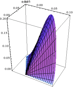 Figure 1
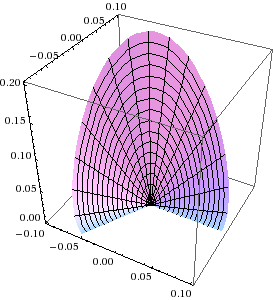 Figure 2
Peer Reviews
No public reviews on file for this paper yet. If you reviewed it on a platform where reviews are public (OpenReview, ICLR, NeurIPS, ICML), you can paste yours below so the community can read it here.
Videos
No videos yet. Explain this paper in a talk, walkthrough, or lecture? Add one.
Taxonomy
TopicsNonlinear Partial Differential Equations · Advanced Mathematical Modeling in Engineering · Numerical methods in inverse problems
Classification of irregular free boundary points
for non-divergence type equations
with discontinuous coefficients
Serena Dipierro
Dipartimento di Matematica, Università degli studi di Milano, Via Saldini 50, 20133 Milan, Italy
,
Aram Karakhanyan
Maxwell Institute for Mathematical Sciences and School of Mathematics, University of Edinburgh, James Clerk Maxwell Building, Peter Guthrie Tait Road, Edinburgh EH9 3FD, United Kingdom
and
Enrico Valdinoci
School of Mathematics and Statistics, University of Melbourne, 813 Swanston Street, Parkville VIC 3010, Australia, and Istituto di Matematica Applicata e Tecnologie Informatiche, Consiglio Nazionale delle Ricerche, Via Ferrata 1, 27100 Pavia, Italy, and Dipartimento di Matematica, Università degli studi di Milano, Via Saldini 50, 20133 Milan, Italy
Abstract.
We provide an integral estimate for a non-divergence (non-variational) form second order elliptic equation , , , with bounded discontinuous coefficients having small BMO norm. We consider the simplest discontinuity of the form at the origin. As an application we show that the free boundary corresponding to the obstacle problem (i.e. when ) cannot be smooth at the points of discontinuity of .
To implement our construction, an integral estimate and a scale invariance will provide the homogeneity of the blow-up sequences, which then can be classified using ODE arguments.
Key words and phrases:
Free boundary, blow-up sequences, non-divergence operators, monotonicity formulae.
2010 Mathematics Subject Classification:
35R35, 35B65
1. Introduction
In this paper we consider the free boundary problem
[TABLE]
with . We will also deal with the case using the notation that identifies to the power zero with the characteristic function .
Problems of this type often arise in real world phenomena. For instance, in the study of the spread of biological populations one studies the problem
[TABLE]
where represents the density of the population, and represents a drift term. Here, , is a positive definite matrix (with entries ) and takes into account the influence of the environment on the population, see [S83].
It is convenient to reformulate the problem in terms of the auxiliary function and write (1.2) as
[TABLE]
Notice that this boils down to the equation in (1.1) when , and with .
The case in which is the identity matrix reduces of course to that of the Laplacian, and, in general, a non-constant models a heterogeneous medium in which the speed of diffusion is different from one point to another.
Moreover, equations in non-divergence form arise naturally from probabilistic considerations, for instance, as the infinitesimal generators of anisotropic random walks, see e.g. Section 2.1.3 in [C08].
Furthermore, when in (1.1) is the identity matrix, the problem is related to the singular one in [AP86], and as it recovers the exemplary free boundary problem in [C77].
One of the main distinctions in the field of partial differential equations consists in the difference between equations “in divergence form” and those “in non-divergence form”. While the first ones naturally admit a variational formulation and can be dealt with by energy methods, the second ones usually require different – and perhaps more sophisticated – techniques (see e.g. [T82] for a detailed discussion), often in combination with viscosity methods.
We refer to [K07, C08] and the references therein for throughout presentations of similarities and differences between equations in divergence and non-divergence form.
A similar distinction between divergence and non-divergence structure occurs in the field of free boundary problems. As a matter of fact, free boundary problems whose partial differential equation is in divergence form often enjoy a special feature given by the so-called “monotonicity formulas”: namely, the energy functional, or a suitable variational integral, possesses a natural monotonicity property with respect to some geometric quantity (typically, a functional defined on balls of radius turns out to be monotone in ).
This type of monotonicity property is, in a sense, geometrically motivated, since it may be seen somehow as an offspring of classical monotonicity formulas arising in the theory of minimal surfaces and geometric flows. In addition, combined with the natural scaling of the problem, a monotonicity formula is often very useful in proving uniqueness of blow-up solutions, classification results and regularity theorems.
Viceversa, problems which do not enjoy monotonicity formulas (or for which a monotonicity formula is not known) may turn out to be considerably harder to deal with, and proving (or disproving) a strong regularity theory is a natural, important and often very challenging question (see e.g. [CS05, PSU12] for further discussions on monotonicity formulas).
The study of free boundary in discontinuous media is also a very active field of research in itself, see in particular [T16] for related problems involving a fully nonlinear dead-core problems, [ALT16] for dead-core problems driven by the infinity Laplacian, and [PT16] for cavity problems in rough media. See also [BT14] for a case in which the coefficients belong to the space of vanishing mean oscillation.
Our objective in the present paper is to study the behavior of the solution of (1.1) near the free boundary points at which the matrix is discontinuous. A model example of this sort in D is
[TABLE]
where is a small constant and (here, we are using the standard notation and ).
One can also write equation (1.3) in the equivalent form
[TABLE]
where
[TABLE]
and
[TABLE]
We observe that the quadratic form
[TABLE]
is positive definite and are discontinuous at the origin.
More generally, we can assume that the diffusion matrix has the form
[TABLE]
where is a homogeneous function of degree zero and for any point we have that
[TABLE]
with
[TABLE]
for some . Roughly speaking, in (1.5), the terms and represent the continuous and the discontinuous parts of , respectively.
Throughout this paper we will assume that the operator satisfies the following conditions:
- (H1)
the entries of the matrix are bounded measurable functions, and the matrix is uniformly elliptic, i.e. there exist two positive constants and such that
[TABLE]
- (H2)
the coefficients have small BMO norm, namely
[TABLE]
where is a small constant.
- (H3)
the matrix has at least one discontinuity at such that is rotational invariant at and homogeneous of degree zero.
In this setting, the problem in (1.1) admits a solution, as given by the following result:
Theorem 1.1**.**
Let , with . Then, there exists a nonnegative function such that , for some , and solves (1.1).
From the technical point of view, concerning the assumptions on the coefficients , we notice that the function for any and . However, if is sufficiently small then holds with , where is a dimensional constant. Consequently, we can apply the estimates from Theorem 4.4 in [CFL93] to establish the existence and optimal growth of the solutions. As a matter of fact, setting
[TABLE]
we can bound the growth from the free boundary according to the following result (see also Theorem 2 in [T16]):
Theorem 1.2**.**
Let be a bounded weak solution of (1.1) in . Then there exists a constant , depending on , such that, for each and any , it holds that .
We remark that the problem in (1.1) has a natural scale invariance: for this, it is useful to define
[TABLE]
with as in (1.6). We notice indeed that is also a solution of (1.1). We will show that, up to a subsequence, these blow-up functions approach a blow-up limit.
We say that is non-degenerate at if there exists a sequence of positive numbers such that the corresponding blow-up limit is not identically zero.
A cornerstone of our analysis is a uniform integral estimate. The result that we obtain is the following:
Theorem 1.3**.**
Let be a strong solution of (1.1) in , with as in (1.4). Assume that and is non-degenerate at [math]. Then
[TABLE]
for some depending on .
In this framework, the integral estimate in (1.7), combined with the scale invariance, implies that the blow-up limits are homogeneous, as described in the following result:
Theorem 1.4**.**
Let be a strong solution of (1.1) in , with as in (1.4). Assume that and is non-degenerate at [math]. Then any blow-up sequence at [math] has a converging subsequence such that the limit is a homogeneous function of degree .
This result will in turn play a special role for the classification of global solutions. Roughly speaking, the homogeneity property, an appropriate use of polar coordinates and explicit methods borrowed from the theory of ordinary differential equations lead to a classification of solutions growing in a non-degenerate way from a smooth free boundary. This classification and the analysis of the blow-up limits will be the main ingredients for the analysis of irregular free boundary points, as explained in the following result (compare also with Corollary 6.8 in [BT14]):
Theorem 1.5**.**
Let , be as in (1.1) and as in (1.4), with sufficiently small. Let be a solution of (1.1) in with . Assume that and that is non-degenerate at [math]. Then cannot be differentiable at the origin.
The paper is organized as follows: in Section 2 we establish the existence of a strong solution of (1.1) in the unit ball and thus prove Theorem 1.1. Next, using a dyadic scaling argument, we prove that a solution grows away from the free boundary as . This is contained in Section 3, which will provide the proof of Theorem 1.2. Our main technical tool, which is the uniform integral bound in Theorem 1.3, is established in Section 4. To this goal, we use some computations based on the ideas of Joel Spruck [S83]. Section 4 also contains the proof of Theorem 1.4, which fully relies on the integral estimate in (1.7). Finally, in Section 5 we show that the free boundary cannot be regular at the free boundary points where suffers a discontinuity satisfying , thus completing the proof of our main result in Theorem 1.5.
2. Existence of solutions
In this section, we give the proof of the existence result in Theorem 1.1.
Proof of Theorem 1.1.
The proof is based on a classical penalization argument. The case of the obstacle problem, corresponding to , is treated in [BT14]. Our proof is similar, but we will sketch it for the reader’s convenience since unlike [BT14] our coefficients are not in VMO. In fact, for our case the proof is shorter since for the penalization function (see below) is continuous at the origin. Hence, by a customary compactness argument, we deduce that the limit of the penalized problem is a solution of (1.1) a.e. Therefore, we only need to establish uniform estimates for the penalized problem (2.5). The details of the proof go as follows.
Let such that , and . Let . Then is a standard mollifier. Set and , where is as in the statement of Theorem 1.1. Furthermore, let be a family of functions with the following properties
[TABLE]
Then, there exists a classical solution to the following Dirichlet problem
[TABLE]
Now, for every , we consider the penalized problem
[TABLE]
Here, the subscript is just a parameter, and does not denote the time derivative. We set
[TABLE]
and we claim that
[TABLE]
Note that , hence by the maximum principle , for some . For any , we consider the operator . Then the Fréchet derivative of is
[TABLE]
Thus the derivative operator has the form
[TABLE]
since, by construction, is monotone increasing. Applying the Schauder theory in Chapter 6 of [GT98], we conclude that for any and there exists a solution of
[TABLE]
This implies that is surjective. By the maximum principle (recall that ) is also injective. Therefore, is invertible, which establishes (2.2).
Now we show that
[TABLE]
To this aim, we first observe that, from the Sobolev embedding, we have that . Consequently, applying the Schauder estimates in Chapter 6 of [GT98], we obtain that
[TABLE]
for some , independently of . Thus if then from Arzela-Ascoli theorem it follows that in and solves the corresponding problem (2.1), thus proving (2.4).
Now, from (2.2) and (2.4), we deduce that a solution of (2.1) exists for all . By Theorem 4.2 in [CFL93], we have that
[TABLE]
uniformly in because verifies -. ∎
3. Optimal growth from the free boundary
Let and consider the scaled function
[TABLE]
We remark that if the inequality
[TABLE]
holds in some neighborhood of , for some constant and as in (1.6), then is uniformly bounded as .
So, we show that the growth control in (3.1) is indeed satisfied for bounded solutions of (1.1). The result that we have is the following:
Proposition 3.1**.**
Let be a weak solution of (1.1) in such that
[TABLE]
for some constant . Then there exists a constant such that for each there holds
[TABLE]
where .
Remark 3.2**.**
It is well known that the estimate in Proposition 3.1 implies the desired growth rate in (3.1).
Proof of Proposition 3.1.
We use a dyadic scaling argument. Suppose that the claim in Proposition 3.1 fails, then there exists a sequence of integers , and points such that
[TABLE]
We introduce the scaled functions
[TABLE]
where is a short notation for . Then, we have that
[TABLE]
and, from (3.3),
[TABLE]
Furthermore, setting , by a direct computation we see that
[TABLE]
Notice also that (3.3) and (1.6) yield that
[TABLE]
Consequently, recalling (3.6), we have that
[TABLE]
Let us define the sequence of matrices . Then satisfies . Observe that the change of variables implies
[TABLE]
Recalling that , we see that
[TABLE]
implying that is also satisfied for the matrices .
Furthermore, in light of (3.7), we see that solves the inequality
[TABLE]
From (3.6), (3.8) and (3.9) it follows that we can apply Theorem 4.1 in [CFL93] to conclude that for any the following estimate holds uniformly in
[TABLE]
where is a fixed ball but with arbitrary radius . Consequently, the sequence of strong solutions is bounded in . From Krylov-Safonov theorem it follows that for a subsequence, still denoted by , we have that in uniformly. Thus and (3.5) translates to the limit function , namely we have
[TABLE]
On the other hand a.e. and satisfies -. In particular, a.e. Hence, and the strong maximum principle imply that which is in contradiction with and the proof is complete. ∎
From Proposition 3.1 and Remark 3.2 we obtain Theorem 1.2, as desired.
4. Blow-up sequences and homogeneity
We want to show that, using a technique invented by J. Spruck in [S83], at the non degenerate free boundary points the blow-up is a homogeneous function of degree . For a sequence of positive numbers and , we consider the blow-up sequence
[TABLE]
From Theorem 1.2 we know that the sequence is bounded and solves equation (1.1) with satisfying -. Thus, applying Theorem 4.1 in [CFL93], we conclude that is locally uniformly bounded in for any . Then a customary compactness argument implies that there exists a subsequence and , such that
[TABLE]
The function is called a blow-up limit at .
4.1. D problems
As customary, it is often useful to write solutions of partial differential equations in polar coordinates. In our case, we have the following result:
Lemma 4.1**.**
Let be as in (1.1), with as in (1.4). Then
[TABLE]
Proof.
We will use polar coordinates , and rewrite the partial derivatives as follows
[TABLE]
By a straightforward computation we have that
[TABLE]
Combining these three identities and recognizing the terms we get that
[TABLE]
Using this and the standard representation of the Laplacian in polar coordinates, the desired result follows. ∎
With this, we are in position of proving Theorem 1.3.
Proof of Theorem 1.3.
We let and . Then we have
[TABLE]
Plugging this into (4.3) we infer that
[TABLE]
This, after recalling that , yields that
[TABLE]
where
[TABLE]
Next, we multiply both sides of equation (4.5) by and we integrate first over the unit circle and then in the interval to get that
[TABLE]
Now we observe that
[TABLE]
Similarly,
[TABLE]
Moreover,
[TABLE]
So, plugging this, (4.7) and (4.8) into (4.6), we obtain that
[TABLE]
Since , the last inequality then reads
[TABLE]
where depends only on the the constant in the growth estimate , see Theorem 1.2. Since and are arbitrary, by the change of variable we obtain that
[TABLE]
This implies the desired result via polar coordinates. ∎
From Theorem 1.3, we obtain the homogeneity of the blow-up sequences, according to Theorem 1.4:
Proof of Theorem 1.4.
By (1.7), a change of variable gives that
[TABLE]
where the notation in (4.1) has been used. This and (4.2) imply that
[TABLE]
and so
[TABLE]
for any , which implies the desired result (see e.g. Lemma 4.2 in [DSV15]). ∎
4.2. -dimensional problems
For the sake of completeness, we consider now a multidimensional model. We take
[TABLE]
Notice that the hypotheses in (H1)-(H3) are satisfied for sufficiently small .
We extend Theorem 1.4 to this case. To this aim, let us switch to polar coordinates and define
[TABLE]
where , with and . In this setting, the analogue of Lemma 4.1 goes as follows:
Lemma 4.2**.**
Let be as in (1.1), with as in (4.9). Assume that lies on the axis. Then
[TABLE]
Proof.
From the chain rule, we have that
[TABLE]
Hence, proceeding as in (4.1), and using to set the point on the axis, we get that
[TABLE]
which gives the desired result. ∎
In this setting, the analogue of Theorem 1.4 is the following:
Theorem 4.3**.**
Let be a strong solution of (1.1) in with as in (4.9). Assume that and is non-degenerate at [math]. Then any blow-up sequence at [math] has a converging subsequence such that the limit is a homogeneous function of degree .
Proof.
We use the change of variables , where is the unit sphere in . Hence, for the function , making use of (4.10), equation (1.1) can be rewritten as
[TABLE]
where is the Laplace-Beltrami operator on the unit sphere. Thus, repeating the integration by parts as in the proof of Theorem 1.3 and the scaling argument in the proof of Theorem 1.4, the desired result follows. ∎
5. Global homogeneous solutions
In this section, we would like to classify the global solutions of (1.1) in the plane in the homogeneous setting for the case of the obstacle problem.
Theorem 5.1**.**
Let , be as in (1.1) and as in (1.4). Let be a solution of (1.1) in with which is homogeneous of degree . Assume that and that is differentiable at the origin. Then in needs to be equal to [math] (and thus ).
Proof.
We first make a general calculation valid for all . Let . We suppose (up to a rotation) that the arc is a component of the positivity set of . In this way,
[TABLE]
We let . From Remark 3.2, we know that (3.1) is satisfied, and thus there exists such that
[TABLE]
For a small , we evaluate this formula at the point , which corresponds in polar coordinate to and . In this way, we obtain that
[TABLE]
So, dividing by and sending , using the fact that ,
[TABLE]
and so
[TABLE]
Furthermore, from (4.3),
[TABLE]
or equivalently
[TABLE]
Multiplying both sides by and integrating yields
[TABLE]
where is an arbitrary constant. Using (5.1) and (5.2), we have that , which gives that . Moreover
[TABLE]
Consequently, solving (5.3) we obtain
[TABLE]
This is a separable equation, and so we obtain
[TABLE]
The integrals above may be explicitly computed in terms of hypergeometric functions for any , but, for concreteness, we now restrict ourselves to the case . In this case, (5.4) becomes
[TABLE]
We now set and we observe that
[TABLE]
Hence, the substitution in (5.5) gives that
[TABLE]
and so
[TABLE]
Then, evaluating (5.6) at and using (5.1), we obtain that
[TABLE]
Thus, defining
[TABLE]
we rewrite (5.6) as
[TABLE]
Since is smooth and homogeneous, formula (5.1) says that , with . Evaluating (5.7) at and , using that (in view of (5.1)), we obtain that
[TABLE]
and therefore . This gives that
[TABLE]
and so
[TABLE]
which, for small , only holds when . ∎
Remark 5.2**.**
From (5.7), one can also construct a homogeneous solution of the obstacle problem in , with as in (1.1) and as in (1.4), whose free boundary is a cone, namely, in polar coordinates, one can take , with
[TABLE]
where and when (respectively, when ), see Figure 1. Notice in particular, that the singular cone of the free boundary can be either obtuse or acute, according to the cases and .
Theorem 1.5 says that this example is somehow “typical”, namely if the free boundary of (1.1) meets the discontinuity points of the coefficients in a non-degenerate way, then a singularity occurs. The proof of this fact is based on Theorem 5.1, and the details go as follows:
Proof of Theorem 1.5.
Assume by contradiction that can be written as a differentiable graph near the origin: say, up to a rotation, that coincides with near the origin, with differentiable, and . We consider the blow-up sequence as in (4.1) (with ). From the discussion at the beginning of Section 4, we know that, for a suitable infinitesimal sequence , it holds that approaches a global solution . Near the origin, we have that coincides with . Using this and the fact that , we thus obtain that near the origin coincides with . Also, from Theorem 1.4, we know that is homogeneous of degree . These considerations and Theorem 5.1 imply that , against our assumptions. ∎
The reference list from the paper itself. Each links out to its DOI / PubMed record.
- 1[AP 86] H. W. Alt, D. Phillips. A free boundary problem for semilinear elliptic equations . J. Reine Angew. Math. 368 (1986), 63–107.
- 2[ALT 16] D. J. Araújo, R. Leitão, E. V. Teixeira. Infinity Laplacian equation with strong absorptions . J. Funct. Anal. 270 (2016), no. 6, 2249–2267.
- 3[BT 14] I. Blank, K. Teka. The Caffarelli alternative in measure for the nondivergence form elliptic obstacle problem with principal coefficients in VMO . Comm. Partial Differential Equations 39 (2014), no. 2, 321–353.
- 4[C 08] X. Cabré. Elliptic PDE’s in probability and geometry: symmetry and regularity of solutions . Discrete Contin. Dyn. Syst. 20 (2008), no. 3, 425–457.
- 5[C 77] L. A. Caffarelli, The regularity of free boundaries in higher dimensions . Acta Math. 139 (1977), no. 3-4, 155–184.
- 6[CS 05] L. Caffarelli, S. Salsa. A geometric approach to free boundary problems . Providence: American Mathematical Society, 2005.
- 7[CFL 93] F. Chiarenza, M. Frasca, P. Longo. W 2 , p superscript 𝑊 2 𝑝 W^{2,p} -solvability of the Dirichlet problem for nondivergence elliptic equations with VMO coefficients . Trans. Amer. Math. Soc. 336 (1993), no. 2, 841–853.
- 8[DSV 15] S. Dipierro, O. Savin, E. Valdinoci. A nonlocal free boundary problem . SIAM J. Math. Anal. 47 (2015), no. 6, 4559–4605.