Generalizations of Divisor Methods to Approval and Score Voting
Martin Djukanovi\'c

TL;DR
This paper extends classical divisor methods like Sainte-Laguë and D'Hondt to approval voting systems, exploring their theoretical foundations and potential generalizations to score voting.
Contribution
It introduces new approval voting methods based on divisor principles and discusses their possible extensions to score voting systems.
Findings
Proposes approval voting methods generalizing Sainte-Laguë and D'Hondt
Analyzes theoretical properties of these methods
Discusses potential for score voting generalizations
Abstract
We introduce several electoral systems for multi-winner elections with approval ballots, generalizing the classical methods of Sainte-Lagu\"e and D'Hondt. Our approach is based on the works of Phragm\'en and Thiele. In the last section we discuss possible generalizations to score voting.
Click any figure to enlarge with its caption.
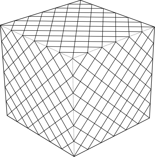 Figure 1
 Figure 2
Peer Reviews
No public reviews on file for this paper yet. If you reviewed it on a platform where reviews are public (OpenReview, ICLR, NeurIPS, ICML), you can paste yours below so the community can read it here.
Videos
No videos yet. Explain this paper in a talk, walkthrough, or lecture? Add one.
Taxonomy
TopicsGame Theory and Voting Systems
Generalizations of Divisor Methods
to Approval and Score Voting
Martin Djukanović The author is grateful to the University of Copenhagen for their hospitality. The author is also grateful to Warren D. Smith and Toby Pereira who provided useful guiding examples. Mathematisch Instituut Leiden,
Institut de Mathématiques de Bordeaux
Abstract
We introduce several electoral systems for multi-winner elections with approval ballots, generalizing the classical methods of Sainte-Laguë and D’Hondt. Our approach is based on the works of Phragmén [5] and Thiele [6]. In the last section we discuss possible generalizations to score voting.
1 A brief overview of divisor methods
Methods of largest quotients, also known as divisor methods,111We shall use these two names interchangeably throughout. are methods of apportionment of seats in parliamentary democracies that use the so called party-list proportional representation. We recall the description of such an electoral system:
- •
The number of seats in the parliament is fixed before the election, but it might vary from election to election.
- •
Only entities known as political parties may participate in the election.
- •
Each political party generates a list of its candidates. This list may be fully or partially public or completely private.
- •
Each election ballot contains the list of political parties participating in the election and each voter must mark exactly one party on the ballot in order to cast a valid vote.
- •
Based on the votes cast, a seat apportionment method proportionally allocates a number of seats to each party and the parties fill their seats sequentially according to their lists.
Let be a finite index set. Let be the set of parties participating in the election and let denote the number of votes that received. Further, let be the total number of votes (i.e. valid ballots) and let be the number of seats to apportion. The rational number is called ’s quota and can be said to be this party’s deserved portion of seats.
The following three are considered desirable properties that a proportional apportionment method should satisfy:
(seat monotonicity) If increases and the votes remain the same, no party should lose a seat in the new apportionment.
- 2)
(vote monotonicity) If increases whilst decreases, then should not lose a seat whilst does not lose a seat or gains a seat in the new apportionment.
- 3)
(meeting quota) Each party should receive either or seats.
It has been known for a long time that divisor methods satisfy the two monotonicity properties but fail to meet quota. Balinski and Young [1] showed that no method can satisfy both 2) and 3) and that only divisor methods satisfy both 1) and 2). They also constructed a method that satisfies both 1) and 3).
Monotonicity in votes is generally considered more important than meeting quota: an increase in support ought to lead to an increase, not decrease, in the number of seats even if it means an occasional unfairness (allocating to some parties strictly less than their lower quota or strictly more than their upper quota). This is the main reason why divisor methods are so widespread and why quota methods have been abandoned in places where they had been used previously. Moreover, empirically, quota violations in divisor methods seem to be rarer than monotonicity violations in quota methods. We now recall the two equivalent definitions of divisor methods.
Definition 1.1** (Largest Quotients Method of Apportionment).**
For , let denote the number of seats that have been allocated to thus far. Initially, set . A largest quotients method allocates the next available seat to the party whose quotient
[TABLE]
is maximal. Here is a monotonically increasing concave function, fixed a priori.
The following, equivalent formulation is probably more intuitive.
Definition 1.2** (Divisor Method of Apportionment).**
For , let denote the quota of party . A divisor method rescales all quotas by a suitable such that
[TABLE]
for some fixed rounding function and allocates seats to party for each .
Remark 1.1**.**
As long as all of the are pairwise distinct, a suitable can be found and the procedure is well defined.
The five classical versions of the method use the following functions:
[TABLE]
The corresponding rounding functions in the divisor formulation can be written as
[TABLE]
where is as follows:
[TABLE]
In other words, after rescaling by an appropriate , the rounding function rounds to either or ; the first method rounds up, the second rounds down, whilst the remaining three round the number down if and only if it is smaller than the arithmetic mean, the geometric mean and the harmonic mean of the two nearest integers, respectively. Ossipoff [8] has suggested , albeit in a different context.
The five classical methods are respectively known as the methods of Adams, Jefferson (a.k.a. D’Hondt), Webster (a.k.a. Sainte-Laguë), Hill (a.k.a. Equal Proportions) and Dean.222These divisor methods were first used for apportioning seats in the US House of Representatives based on state populations and they are named after their inventors. They were later rediscovered in Europe, as methods of largest quotients, where they are known under different names. The most commonly used variants are D’Hondt and Sainte-Laguë. They are usually formulated as follows: divide all of the by a sequence of increasing numbers and allocate the seats to the parties that correspond to the largest quotients. The D’Hondt sequence is , whereas the Sainte-Laguë sequence is . These can be modified easily to tweak the properties of the method; e.g. the sequence is used in some countries with the intent of making it more difficult for parties to win their first seat.
Note that the Adams method has an obvious bias towards smaller parties, whilst the Jefferson/D’Hondt method has an obvious bias towards larger parties. The D’Hondt method is nevertheless used throughout Europe (and elsewhere) for various reasons.333It encourages formation of large parties and coalitions, supposedly leading to more stability. It also meets the lower quota, awarding at least seats to . The Sainte-Laguë variant is arguably the fairest among these five because it sequentially minimizes the variance of the number of representatives per voter, making representations as even as possible. On the other hand, D’Hondt only minimizes the amount of representation of the voter with the most representation. Empirically, the Sainte-Laguë method seems to violate quota less often than the other four methods.
2 Approval and score voting
Consider a single-winner election with two candidates, and . The best method of choosing the winner in this election is the obvious one – the winner is the candidate with the majority of the votes (cf. May’s theorem [2]). This simple election can be generalized to elections with more than two candidates and those can be further generalized to elections with more than one winner. We briefly recall the different approaches to the first step in the generalization.
- •
The simplest generalization to the case of more than two candidates imposes the condition that the voter must choose exactly one candidate to support. The candidate with the most votes is the winner; this is known as plurality rule. This method does not permit the voter to express that she does not consider the candidates she did not vote for to be equally bad or that she considers some of them to be at least as good as the one she did vote for, leading to well known problems in practice, such as dishonestly choosing “the lesser of two evils” so as not to split the vote against the greater evil.
- •
One approach, which may be called the Condorcet approach, interprets a vote for instead of as a statement of “preference for over ”, denoted . If one increases the number of candidates, this is then generalized to a preference chain . The winner of such an election is declared to be the candidate who would pairwise beat any other candidate (in an election comparing preferences for one over the other), if such a candidate exists. Such a candidate is called the Condorcet winner and a method that always elects the Condorcet winner, if one exists, is called a Condorcet method. Many such methods have been developed and they differ in how they treat the case when there is no Condorcet winner. While they satisfy many interesting properties, they are not free of paradoxes (cf. Arrow’s theorem [3]) and they are usually computationally demanding. We consider Condorcet methods too deficient to be used for electing state officials and we do not discuss them further.
- •
Another generalization interprets a ballot in the vs election as splitting the candidates into two subsets, namely those that the voter approves and those that the voter does not approve. This has an obvious generalization known as approval voting – the voter marks the candidate(s) she approves and the most approved candidate wins.
- •
One can also interpret a ballot in the vs election as giving the worst candidate a score of zero and giving the best candidate a score of one. This is then generalized to giving every candidate some score and is known as score voting (or range voting). The candidate with the highest total score wins the election. Not every possible score may be given in practice, however. Instead, for simplicity, the only scores that may be awarded are
[TABLE]
for some fixed . The method can be modified slightly to allow votes of no opinion, but this is not something we shall be dealing with in this paper.
Remark 2.1**.**
In Score, there is an incentive for voters to maximize the impact of their vote by strategically awarding only scores of either zero or one. Since not all voters would use this to their advantage, it is sometimes argued that zero and one should be the only scores allowed, i.e. that Approval should always be used instead of Score. We contend that voters should always have the choice of awarding “suboptimal” scores.
There are various other, exotic methods, but we do not discuss them here. Advantages and disadvantages of each are discussed at length elsewhere. We hold that score voting has numerous advantages over other methods, in terms of application to elections of state officials. A detailed list of these can be found at [4]. Whether or not the reader agrees with this view, it is the reason behind our endeavor to generalize Score to multi-winner elections. Our goal in this paper is to introduce particular natural generalizations that combine Approval/Score with the method of largest quotients. We wish for them to be scrutinized, improved upon, and compared with other methods.
3 A generalization of Sainte-Laguë to Approval
We abandon entirely the party-list approach and consider an election with approval ballots in which the voter is free to mark any candidate she approves, regardless of party affiliation. From now on, shall denote the number of candidates, shall denote the number of voters, and shall denote the number of seats to apportion. The number of seats is essentially irrelevant because the method orders the candidates independently of this number444However, one can choose divisors that depend on the number of seats (see [7]) or even the number of allocated seats. and then fills the seats sequentially, according to the ordering. The ballots can be considered to be given in the form of an binary matrix where
[TABLE]
We refer to the rows of this matrix as candidates, denoting them by , and we refer to the columns as voters. Identical candidates are referred to as clones.
After permuting the columns if necessary, the usual “choose one party-list” election corresponds to a matrix of the following form:
[TABLE]
where the omitted values are all zeros. In other words, in the usual scenario, any two candidates are forced to be either clones or orthogonal. Recall that Sainte-Laguë awards the next available seat to the candidate whose quotient
[TABLE]
is maximal. The integer is the number of votes for (and all its party clones) and may be denoted by
[TABLE]
The integer is the number of clones of that have already been elected and it can be interpreted as the number of seats that are already representing the supporters of . Removing the choose-one-party-list restriction and allowing the ballot matrix to be any binary matrix of size , we can generalize and in a natural way. If a candidate is elected and , we consider that the seat of is equally split among the -voters; each one is considered to be represented by of the seat. This leads us to the definition of Algorithm 1.
We fix some notations first. We shall denote by the usual scalar product, whilst
[TABLE]
shall denote the - and -norms, respectively. For a finite set of non-zero points in , we shall denote by the sum of their normalizations with respect to the -norm, that is
[TABLE]
If then by convention. We shall use the words set and list interchangeably when referring to the elected candidates as it is not always relevant that the candidates are elected in a specific order.
Algorithm 1** (“Phragmén-Sainte-Laguë”).**
Let be the empty list. As long as there are candidates not on the list, append to it the candidate with the maximal quotient
[TABLE]
The list gives the ordering of the candidates. Ties are broken by index (which is assumed to be pseudo-random in practice).
Note that since , the first candidate on the list is always the most approved one. This algorithm is precisely the greedy algorithm that sequentially minimizes the variance of the number of representatives per voter for each seat it allocates (Proposition 3.1). When applied to the party-list scenario, this is just the usual Sainte-Laguë method.
Proposition 3.1**.**
Algorithm 1 minimizes the variance of voter representation for each seat it allocates (assuming candidates with zero approval are ignored).
**Proof ** Assume that there are no candidates with zero approval. Voter representations are given at each step by the vector and its variance is, by definition, the square of its -distance from the ideal representations (that are given by the vector with the arithmetic mean of in each coordinate), divided by , i.e. if candidates have been elected then
[TABLE]
Suppose, without loss of generality, that . Then it is readily seen that
[TABLE]
It follows that is minimal precisely when is chosen so that
[TABLE]
is maximal. Since , we have and the claim follows. ∎
This method has some obvious issues. One could say that it considers voter equality more important than candidate quality (i.e. popularity). Since we allow non-identical candidates to have common supporters, it is difficult to say to whom a particular candidate “belongs” – a candidate can be shared by different groups. This can lead to a situation where the method considers a “moderate” candidate, shared between two groups, worse than an “extreme” candidate, supported by just one of the groups, because electing the moderate might over-represent one of the groups. This can be thought of as a kind of Pareto inefficiency: a candidate is elected even though there is a more popular candidate that is approved by all (or most) of the -voters. We elaborate on this in the examples that follow.
Example 3.1**.**
Let be an integer. Consider the following distribution of approvals in an election:
[TABLE]
Algorithm 1 gives the ordering because allocating the second seat to would give the -voter too much representation; is orthogonal to , so represents the voters more evenly. This is in spite of the fact that is a Pareto improvement over ; every -voter is also a -voter but not the other way around.
Would it be a good idea to give the second seat to ? That depends on whether or not one considers voter approval (and voter representation to an extent) as a sort of welfare in the sense that increasing it for some does not harm others. On one hand, one can argue that if a group is over-represented, the parliament is biased. On the other hand, it counters intuition that some unpopular candidates should be overlooked only because some of their supporters also support some popular candidates. We hold it reasonable that small groups should not be discouraged from supporting some popular candidates over others in order to, as it were, swing the first allocated seats towards their side.
Remark 3.1**.**
A method cannot be considered fair if it places too much importance on popularity. In the extreme case, we could have a plurality-type method that simply awards all of the seats to the clones of the most popular candidate, provided that there are sufficiently many of them running. The same is true at the other end of the spectrum. Consider an example such as:
[TABLE]
If we are to apportion exactly seats, then the most proportional outcome would be to elect the . However, this completely ignores the fact that is universally approved. It is therefore not a good idea to place too much importance on proportionality either.
The following is an example in a spirit similar to Example 3.1.
Example 3.2**.**
Let be an integer. Consider the following distribution of approvals:
[TABLE]
Algorithm 1 gives , regardless of , even though is a Pareto improvement over . One could alter the method so that it checks for Pareto improvements at each step. However, if we suppose that is large and we add one voter who approves only , we have voters who prefer to and only one voter with the opposite preference. Then, even though is no longer a Pareto improvement over in the strict sense, one is tempted to elect over and argue that the opinion of the voters matters more than the opinion of the single voter with the opposite preference. The question is, how many supporters of need to be added before this decision is reversed?
In the next section, we present a method that aims to deal with this issue.
4 Improving the simple generalization
The usual party-list divisor methods are a special case in which the number of voters who support candidate but not candidate is either or zero. Another way of describing the election procedure in that scenario is as follows. Consider all possible pairs of candidates that have not been awarded a seat thus far and define a relation for each step in the algorithm, i.e. for each seat to be filled, by the condition
[TABLE]
where is the number of voters who approve but not and is the number of seats that represent these voters. The next available seat is given to a candidate such that for every . Ties occur when , when both quotients are zero, and they are broken by the party-list. Perhaps one could generalize to Approval from this point of view by defining the relation by the condition
[TABLE]
with being the set of candidates elected thus far and
[TABLE]
In other words, and its -th coordinate is given by
[TABLE]
However, this relation is not transitive in general and cycles can occur. One could consider applying a Condorcet method at this point, but we do not pursue that idea. Instead, we define the following method.
Algorithm 2** (“Pareto-improved Phragmén-Sainte-Laguë”).**
Let be the empty list and let denote the set of candidates. As long as there are candidates not on the list, do the following:
Find the candidate with the maximal quotient
[TABLE]
- 2)
If the set
[TABLE]
is empty, then append to , otherwise append for which the difference
[TABLE]
is maximal.
The list gives the ordering of the candidates. A tie in step 1) is broken by comparing the quotients defined in step 2) (in favour of rather than if gives a larger quotient than ) and if the quotients in step 2) are equal, the tie is broken by index.
In particular, a candidate will always be considered worse than a candidate that Pareto-dominates , if such a candidate exists. When applied to Example 3.2, this method gives the ordering
[TABLE]
and it takes exactly additional voters who approve only to change this ordering back to
[TABLE]
However, this method is not free of issues. The aim of step 2) is to improve upon the candidate from step 1). Of course, it matters which candidate the improvement is based upon and it might happen that one group of voters “hijacks” a candidate from another group.
Example 4.1**.**
Let the following matrix represent the distribution of approvals in an election.
[TABLE]
The first four voters approve only the candidates and, from their perspective, the two groups of candidates can be thought of as parties. The method awards the first seat to , it being the most popular candidate, with ten approval votes. We accordingly set
[TABLE]
The next seat goes to a candidate that maximizes
[TABLE]
There are three such candidates, namely , , and . In the second step, and are tied and both beat so wins the second seat and we set
[TABLE]
Step 2) of the algorithm does not give any improvements over . Continuing in this way, the first four seats are awarded to , , , , in that order, without any improvements in step 2). Before the fifth seat is allocated, we have
[TABLE]
and
[TABLE]
so is the fairest choice for the fifth seat. Recall that the vectors
[TABLE]
denote the voters with preferences and , respectively. Since
[TABLE]
and is the only available candidate for which such an inequality holds with respect to , candidate is elected next. This is in spite of the fact that according to (4.3), electing is considered more proportional. We could say that candidate almost Pareto-dominates candidate ; there is a single voter who prefers over , but she is not sufficiently under-represented to justify electing . Similarly, before the sixth seat is allocated we have
[TABLE]
and we check that
[TABLE]
However, we also have
[TABLE]
and therefore candidate is elected next even though, according to (4.4), electing would be more proportional. However, if we suppose that only the first four voters voted for , the situation changes. To illustrate the point, suppose that we added a candidate to the election. Then would be considered the best at step 1) for the sixth seat. However, at step 2), candidate would be considered an improvement over and would not, so would be elected instead.
Remark 4.1**.**
It is difficult to say to what extent this would be a problem in practice, however. It is certainly possible for a voter to approve certain winners, accumulate enough representation, and cast a vote of approval that harms a relatively unpopular candidate. In particular
[TABLE]
Introducing step 2) with helps the situation somewhat because . One idea worth considering might be the addition of placeholder phantom candidates, such that each voter can vote for only one such candidate. These candidates would be present only so that they could be chosen in step 1) for improvement in step 2) and would be ineligible otherwise. The intended effect is similar to the effect of adding in the example above. This could be accomplished by merging the ballot with the traditional choose-one-party ballot that contains the list of registered parties and the option None available to the independents, who would not have a phantom candidate of their own. However, we are still left with the possibility of larger parties intentionally hijacking the phantom candidates of smaller parties.
Remark 4.2**.**
The underlying philosophy of this method, and the sense in which it is a generalization of party-list divisor methods, can be stated as follows: determine which party is to receive the next seat and then give the seat to the best candidate of that party. The word party is understood as a group of like-minded voters, not candidates. The method itself determines the “parties” and the “party-lists”, as it were. The variant with phantom candidates is guided towards the actual parties. Other variants of the method can be obtained by replacing the corresponding divisors by the various other possibilities mentioned in the first section. Moreover, different divisors can be used in steps 1) and 2).
5 Thiele, Phragmén and a new approach
Phragmén’s method [5], properly interpreted, turns out to be the D’Hondt variant of the method described by Algorithm 1. It also uses the vector , whose coordinates Phragmén calls loads, a name that is perhaps a better choice than ours. In this method, the candidate who wins the next available seat is the candidate whose supporters would have the minimal average load after is elected. If is the list of candidates elected thus far, Phragmén elects that minimizes
[TABLE]
which is to say that maximizes
[TABLE]
which is clearly a generalization of D’Hondt.
Thiele’s method [6] works by assigning weights to the ballots. For each seat to be filled, each voter’s ballot is first divided by , where is the number of elected candidates that the -th voter approved, and the seat is given to the candidate with the highest total score after summing the reweighted ballots. Instead of dividing by , it is also possible to define the method by divisors etc. Note that Thiele’s method also generalizes D’Hondt and Sainte-Laguë to Approval (depending on which divisors are chosen). However, Thiele’s method is deficient in one important way: it strongly encourages the voters not to approve the candidates who are most probably going to be elected even without their support. Withholding such unnecessary support would increase significantly the impact of their vote when electing less popular candidates. This issue is less pronounced with Phragmén.
Remark 5.1** (Nomenclature).**
With the history in mind, we suggest that the classical method of Phragmén, as defined here, be referred to as Phragmén-D’Hondt and that the method given by Algorithm 1 be referred to as Phragmén-Sainte-Laguë (or respectively as the D’Hondt and the Sainte-Laguë variants of Phragmén’s method). The improved method based on “difference quotients”, given by Algorithm 2, might be named after the differences or referred to as Pareto-improved Phragmén (Sainte-Laguë variant as given in the definition, with obvious modifications to obtain other variants). We suggest analogous names for the corresponding variants of Thiele’s method.
The key difference between Phragmén and Thiele lies in how they treat the notion of the amount of representation that a voter has and how that amount influences the election procedure. Under Thiele, if some voters approved an elected candidate, they are considered to be represented by that candidate. Under Phragmén, they are considered to be represented by the candidate only to the extent that they contributed to getting said candidate elected. Note that Phragmén can be interpreted as a method that reweights the votes of like-minded voters by the same amount and then compares the candidates’ total scores. Both methods reweight the votes in a way that can be seen as unfair towards small groups. Thiele reweights the entire ballot and does so without considering the popularity of elected candidates, whilst Phragmén reweights a vote for a particular candidate on a voter’s ballot based almost entirely on the previous choices of other supporters of that candidate.
Example 5.1** (Example 4.1 revisited).**
If we put , changing the votes of the third and the fourth voter, then the position of is improved under both Phragmén and Thiele, in both the classical variants and the variants with differences (using for purposes of Pareto improvements in Thiele’s method, where denotes the candidate with coordinates reweighted with respect to the set of elected candidates using Sainte-Laguë divisors).
Note that Thiele always reweights the columns of the ballot matrix by a fixed amount, whereas Phragmén reweights the rows by a fixed amount (see also Example 5.2). This suggests that a reasonable Approval method might be obtained by combining the two approaches. In what follows, we present one such method and its corresponding Pareto-improved variant.
Our goal is to reweight the entries in the ballot matrix individually instead of reweighting a row or a column by a fixed amount. We wish to do so in a way that only considers individual representations, not collective (like Phragmén), and a way that is not excessively harsh towards small groups (like Thiele is).
Consider again the case of the choose-one-party-list election, this time from the points of view of Phragmén and Thiele. If at some step in the election procedure a voter of has representation , that is simply to say that the party with votes has won seats thus far. For the purpose of reweighting, Thiele comes up with as the number of summands in
[TABLE]
counting how many times this voter has obtained some positive amount of representation. In the general case, Thiele reweights the entire ballot without taking into account the actual amounts. On the other hand, Phragmén comes up with by summing the individual representations of the voters who approved the next available -clone on the party list. These are precisely the voters with representation each and we have
[TABLE]
In the general case, Phragmén reweights all votes for a candidate equally, without taking into account the individual contributions to the total amount of representation that the supporters of the candidate have.
To meet our goal, we suggest that be interpreted as the product of the current representation of the -voter and the number of votes for the -candidate:
[TABLE]
Equivalently, this can be seen as the ratio of the amount of representation that the -voter currently has and the amount that she would receive if one of the -candidates was elected next, i.e.
[TABLE]
In the general case, dropping the - prefix, this approach would treat like-minded groups corresponding to clones (resp. near-clones) much like Sainte-Laguë, dividing precisely (resp. approximately) by as they got elected and, at the same time, it would not punish excessively any small groups that have partial agreement with larger groups. We introduce the necessary notation before writing down the formal definition.
For any and we denote by the point with coordinates reweighted with respect to in the sense above, based on (5.1). That is to say that
[TABLE]
For later convenience, we also introduce
[TABLE]
for any . Note that for we have .
Algorithm 3**.**
Let be the empty list and let denote the set of candidates. As long as there are candidates not on the list, append to it the candidate with the maximal norm The list gives the ordering of the candidates. Ties are broken by index.
Algorithm 4**.**
Let be the empty list and let denote the set of candidates. As long as there are candidates not on the list, do the following:
Find the candidate for which the norm is maximal.
- 2)
If the set
[TABLE]
is empty, then append to , otherwise append for which the difference
[TABLE]
is maximal.
The list gives the ordering of the candidates. A tie in step 1) is broken by comparing the norms defined in step 2) (in favour of rather than if ) and if the norms in step 2) are equal, the tie is broken by index.
Note that reweights an individual vote for based only on the popularity of and the individual representation of the voter, and that the method is free of artificial constructions such as phantoms etc. It is clear how other variants, such as D’Hondt, can be obtained by modifying (5.3) and (5.4).
When applied to Example 3.2, Algorithms 3 and 4 give the same result as the two Phragmén algorithms, but now only additional -voters are needed for Algorithm 4 to elect over .
Example 5.2** (Example 4.1 revisited).**
To see more clearly the difference between Thiele, Phragmén and Algorithm 3 (all in Sainte-Laguë variants), we take a look at the reweighted ballot matrix in each method when . In Thiele we have
[TABLE]
in Phragmén we have
[TABLE]
and in Algorithm 3 we have
[TABLE]
When applied to Example 4.1, Algorithms 3 and 4 respectively give
[TABLE]
If we set then they respectively give
[TABLE]
If , Algorithm 4 gives .
Remark 5.2**.**
Like Phragmén and Thiele, both of these algorithms are not monotonic; changing a vote from [math] to can lower the position of the corresponding candidate, as can be seen by changing the first vote of the first voter in the following two ballot matrices:
[TABLE]
6 A geometric interpretation and generalizations to Score
It is natural to ask whether one can generalize these methods to Score. One immediate generalization is obtained by converting the scores to approval votes. If the allowed scores in are integer multiples of for some , then we can treat every score voter as approval voters and convert the scores via
[TABLE]
However, one hopes to obtain a direct generalization by allowing votes between zero and one in Approval. We make a few observations.
There are infinitely many ways to continuously fill the gap between zero and one and it need not be done linearly. Unlike Approval, Score allows for the total score of a candidate to arise in many different ways from the voters supporting (the voters who gave non-zero scores). The question is whether all these possibilities should be treated equally and whether the scores should simply be summed when comparing candidates. For example, one could argue that a hundred voters, each of whom contributed a score of , should not be treated the same as one voter who contributed a score of 1. If these were the scores of two candidates, it could be that some of the hundred voters would be willing to change their scores to zero so that the voter with the opposite preference, who is much more passionate about her choice, can have her way. It is not clear how this should be treated. One might, for example, apply a transformation to the scores , such as or with , chosen so that , etc.
If a candidate is elected, one can argue that its contribution to voter representations should be given by , with multiplication defined coordinate-wise. For example, if voters give a score of , each portion that is of the filled seat can be said to be worth only of that amount to each voter, whence . The same conclusion can be reached by considering the representations after the conversion given by (6.1).
Whether the representations are given by or , a method that simply minimizes representation variance is not a good method because a candidate with a low score is considered good if the voters agree very much on how bad the candidate is. It is also not a good idea to simply minimize the distance from the ideal representation . For example, the distance between and approaches 0 as , whereas the distance between and approaches 1. A consistent generalization should not only prefer lower variance in the number of seats per voter, it should also prefer higher candidate scores. Moreover, if we impose the condition that equal total scores should be considered equally good, all else being equal, this introduces additional difficulties.
6.1 Generalizing Phragmén
Consider again an election with approval votes. Phragmén-D’Hondt and Phragmén-Sainte-Laguë can be interpreted as different takes on a particular optimization problem. Let us normalize the candidates with respect to the -norm and set
[TABLE]
so that each is a point in the standard -simplex
[TABLE]
Since , the normalized are actually midpoints of faces (of various dimensions) of the simplex . Clearly, the sum of any normalized candidates is a point in the rescaled simplex . If we are given the set , we can interpret the Phragmén method as the greedy algorithm that sequentially chooses points from in such a way that at the -th step the distance between the sum of the chosen points and is minimal. Since is orthogonal to the line , the same quality measure can be defined by the distance from or by the distance from some point . Note that starts at the origin and moves through the cone defined by as the seats are filled. One hopes to generalize this method to Score by generalizing the normalization function and then defining a similar problem. If one were to use as individual amounts of representation and minimize the distance between and a point , it would not be clear how should be chosen and how it should change in different steps of the algorithm, if at all. A more distant reference point would discriminate more against lower scores.
In what follows, we describe a somewhat plausible approach. Note that the votes in Approval correspond to vertices of the unit hypercube . Instead of assuming that the candidates in Score are arbitrary points in , we shall impose a slight limitation by assuming that all candidates lie on the facets of that contain . In other words, we assume that every candidate has at least one coordinate equal to 1. This clearly generalizes Approval where the same assumption means that there are no candidates with . The normalization function
[TABLE]
used in Approval, maps the facets containing to the simplex . Let . Imposing the condition that, on the first step, equal total scores should be treated equally, we replace by where
[TABLE]
We set . This generalizes Approval as it is readily seen that
[TABLE]
if has exactly coordinates equal to 1. See Figure 1 for an illustration of this new normalization function.
A method that sequentially chooses by minimizing generalizes Phragmén-Sainte-Laguë, but to carry out the improvement with the difference quotients, analogous to the one in Algorithm 2, we will also assume that the difference has at least one coordinate equal to 1 for any two candidates . We can ensure this by adding at least one phantom voter per candidate that gives that candidate a score of 1 and a score of 0 to every other candidate. This limits the applications of the method as it is necessary to assume that is significantly larger than , so that this modification does not bias the result of the election too much. It is reasonable to assume that in parliamentary elections. In such elections, the phantom voters could be the candidates themselves, i.e. the phantom voters could be added and the candidates disfranchised. Alternatively, the phantom voters could be apportioned (based on polls, signatures, previous results etc.) by a divisor method that guarantees at least one phantom voter per candidate.
Before we write down the formal definition, we remark that is still defined as in (4.1):
[TABLE]
for any and . We will need to introduce a new vector to replace . To that end, for a finite set of points on the facets of away from the origin, let
[TABLE]
with the convention .
Algorithm 5** (A generalization of 1).**
Let be the empty list and let be the set of candidates such that every has at least one coordinate equal to 1. As long as there are candidates not on the list, append to it the candidate that minimizes
[TABLE]
The list gives the ordering of the candidates. Ties are broken by index.
Algorithm 6** (A generalization of 2).**
Let be the empty list and let be the set of candidates such that has at least one coordinate equal to 1 for every . As long as there are candidates not on the list, do the following:
Find the candidate for which is minimal.
- 2)
If the set
[TABLE]
is empty, then append to , otherwise append that maximizes
[TABLE]
where is the number of candidates elected thus far.
The list gives the ordering of the candidates. A tie in step 1) is broken by comparing the norms in step 2) that define and if they are equal, the tie is broken by index.
Remark 6.1**.**
Expression (6.2) is chosen so that it generalizes (4.2), which is understood as the difference of the sums of the reweighted votes. This is by no means a canonical choice; many different variants of the method can be defined by choosing a different candidate as the best improvement in the set .
We make several observations about this approach. As we have seen, when restricted to Approval, is the difference between the ideal and the representations that the voters receive if is elected. The sum
[TABLE]
of these differences can be interpreted as the overall bias of the elected set . In Score, no longer corresponds to an intuitive definition of over-representation, but can still be interpreted as a “bias-vector” associated to .
Example 6.1**.**
Let be a positive integer such that and let
[TABLE]
Then . Consider the following classical special case. Let and suppose that there are two seats to apportion and that a candidate is given the first seat. The classical Sainte-Laguë method considers that there is a tie for the second seat between a clone and . However, both of these choices are suboptimal in the sense that representations
[TABLE]
deviate from the ideal values (by an equal amount but in different directions). However, measuring bias by , the ideal candidate for the second seat would be
[TABLE]
because the two elected candidates would have an equal number of votes “in opposite directions”.
Example 6.2**.**
Let be a positive integer such that and let
[TABLE]
where
[TABLE]
Then . In particular, under , the two sets
[TABLE]
are considered equally biased against the third voter.
One hopes that examples like these will provide useful insight into the nature of the methods given by Algorithms 5 and 6.
6.2 Generalizing the new method
There is more than one way to generalize Algorithms 3 and 4 to Score and we will present two simple generalizations. We change the definition of voter representation in both cases; if is the set of candidates elected thus far, we set
[TABLE]
Algorithm 7**.**
Apply Algorithm 3 using definitions (6.3) and (5.3).
Algorithm 8**.**
Apply Algorithm 4 using definitions (6.3), (5.3) and (5.4).
The second approach generalizes the reweighting function in a way that is consistent with (5.2). Specifically, for any , the -th coordinate of is now defined as
[TABLE]
Similarly, we redefine
[TABLE]
Algorithm 9**.**
Apply Algorithm 3 using definitions (6.3) and (6.4).
Algorithm 10**.**
Apply Algorithm 4 using definitions (6.3), (6.4) and (6.5).
6.3 Examples
Finally, to point out the differences between the methods, we provide two examples with scores in , with phantom voters added. Algorithms 1, 2, 3 and 4 are applied after converting the scores to approval votes via (6.1).
Example 6.3**.**
For
[TABLE]
we get the following outcomes:
- •
Algorithm 1:
- •
Algorithm 2:
- •
Algorithm 3:
- •
Algorithm 4:
- •
Algorithm 5:
- •
Algorithm 6:
- •
Algorithm 7:
- •
Algorithm 8:
- •
Algorithm 9:
- •
Algorithm 10:
Example 6.4**.**
For
[TABLE]
we get the following outcomes:
- •
Algorithm 1:
- •
Algorithm 2:
- •
Algorithm 3:
- •
Algorithm 4:
- •
Algorithm 5:
- •
Algorithm 6:
- •
Algorithm 7:
- •
Algorithm 8:
- •
Algorithm 9:
- •
Algorithm 10:
The reference list from the paper itself. Each links out to its DOI / PubMed record.
- 1[1] Michel L. Balinski and H. Peyton Young, Fair Representation: Meeting the Ideal of One Man, One Vote (2nd ed.) , Brookings Institution Press (2001) ISBN: 9780815701118
- 2[2] Kenneth O. May, A Set of Independent Necessary and Sufficient Conditions for Simple Majority Decisions , Econometrica, Vol. 20, Issue 4, pp. 680–684 (1952) JSTOR: 1907651
- 3[3] Kenneth J. Arrow, A Difficulty in the Concept of Social Welfare , Journal of Political Economy, Vol. 58, Issue 4, pp. 328–346 (1950) DOI: 10.1086/256963 · doi ↗
- 4[4] http://rangevoting.org
- 5[5] Lars E. Phragmén, Till Frågan om en Proportionell Valmetod , Statsvetenskaplig Tidskrift Vol. 2, Issue 2, pp. 87–95 (1899) Facsimile: http://scorevoting.net/Phragmen Voting 1899.pdf
- 6[6] Thorvald N. Thiele, Om Flerfoldsvalg , Oversigt over Det Kgl. Danske Videnskabernes Selskabs Forhandlinger, Res. XV-XVIII, pp. 415–441 (1895) Google Books: o AMXAAAAYAAJ ; Jahrbuch Database: JFM 26.0254.01
- 7[7] Warren D. Smith and Michael Ossipoff, private communication (2007) http://www.rangevoting.org/New Appo.html
- 8[8] Michael Ossipoff, private communication (2006–2007) election-methods mailing list