The Curie-Weiss model with complex temperature: phase transitions
Mira Shamis, Ofer Zeitouni

TL;DR
This paper investigates the behavior of the Curie-Weiss model when the temperature parameter is complex, analyzing phase transitions and the zeros of the partition function to deepen understanding of its mathematical properties.
Contribution
It provides a partial description of phase transitions and the distribution of zeros of the partition function for the complex-temperature Curie-Weiss model, extending classical results.
Findings
Identification of phase transition regions in the complex temperature plane
Characterization of the zeros of the partition function
Insights into the analytic structure of the free energy
Abstract
We study the partition function and free energy of the Curie-Weiss model with complex temperature, and partially describe its phase transitions. As a consequence, we obtain information on the locations of zeros of the partition function.
Click any figure to enlarge with its caption.
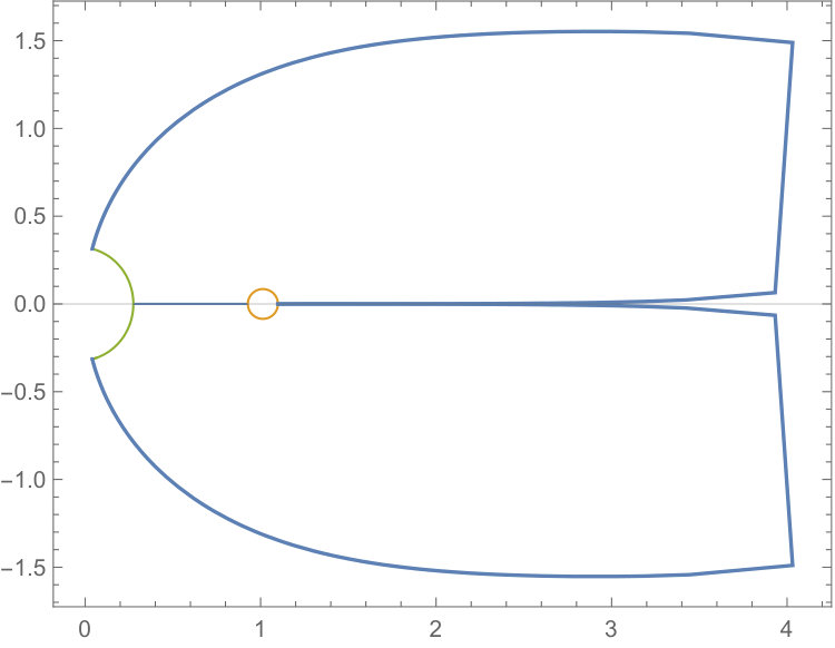 Figure 1
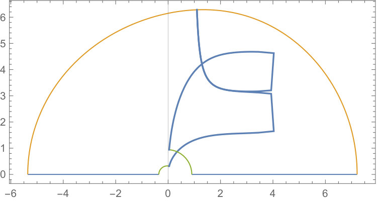 Figure 2
 Figure 3
 Figure 4
Peer Reviews
No public reviews on file for this paper yet. If you reviewed it on a platform where reviews are public (OpenReview, ICLR, NeurIPS, ICML), you can paste yours below so the community can read it here.
Videos
No videos yet. Explain this paper in a talk, walkthrough, or lecture? Add one.
11footnotetext: Department of Mathematics, Weizmann Institute of Science, Rehovot 7610001, Israel and School of Mathematical Sciences, Queen Mary University of London, Mile End Road, London E1 4NS, England. E-mail: [email protected]. Supported in part by ISF grant 147/15.22footnotetext: Department of Mathematics, Weizmann Institute of Science, Rehovot 7610001, Israel. E-mail: [email protected]. Supported in part by ISF grant 147/15. This project has received funding from the European Research Council (ERC) under the European Union s Horizon 2020 research and innovation programme (grant agreement No. 692452).
The Curie–Weiss model with complex temperature: phase transitions
Mira Shamis1, Ofer Zeitouni2
Abstract
We study the partition function of the Curie–Weiss model with complex temperature, and partially describe its phase transitions. As a consequence, we obtain information on the locations of zeros of the partition function (the Fisher zeros).
1 Introduction
An important component of large deviations theory is Varadhan’s lemma, which states that if a sequence of probability measures satisfies the large deviations principle in a (Polish) space with speed and rate function , then for any bounded continuous function ,
[TABLE]
See [2] for a precise statement, relaxed assumptions, and applications.
In many applications, considering real-valued is too restrictive, and one may be interested in relaxing it to allow for complex-valued . Statistical mechanics provides for a rich class of examples; we mention in particular the Yang–Lee theory [11], where the complex perturbation is in form of a magnetic field, or the quantum spin chain models [7], where quantitites of interest such as emptiness formation can be formulated as exponential asymptotics of the type (1.1) with complex integrand. Note that in such examples, because is multiplied by , relatively small changes in phase may lead to sign changes of the integrand in (1.1) and therefore to cancelations.
It seems maybe naive at this point to hope for a general theory, which would consist of an analogue of (1.1). Our goal in this paper is more modest: we consider one simple example, the Curie–Weiss model with complex temperature, and partially develop the asymptotic theory concerning its partition function. While we are not able to give a complete description of the associated phase diagram, we will be able to show that the phase diagram is not trivial. As a consequence of our analysis, we will also obtain information on the (complex) zeros of the partition function, which are called the Fisher zeros; see [4] for a discussion of the relations between these zeros and various critical exponents.
The Curie–Weiss model at complex temperature was also recently considered by Krasnytska et al. [6]; the focus of their work is on the Fisher zeros in the vicinity of the critical point. We further comment on their results at the end of this introduction.
We begin by introducing the Curie–Weiss model that we will consider. Let . Define the Hamiltonian
[TABLE]
where the magnetization is . For , let denote the partition function, i.e.
[TABLE]
where .
When is real, it is an easy exercise to apply Varadhan’s lemma (1.1) and Cramer’s theorem concerning the large deviations of in order to conclude that
[TABLE]
where is the free energy. More refined analysis (see e.g. [3]) yields that for ,
[TABLE]
where is some constant that depends only on ; this is due to the Gaussian nature of the fluctuations of , where is the asymptotic magnetization, under the measure . Also, for .
Remark 1.1**.**
Here and throughout the paper, the notation and is used for asymptotics as , for fixed . That is, if and if the last equals [math]. When we want to emphasize dependence on other parameters, we use the notation , etc.
When , one expects to similarly have a separation between a region where and . In particular, one predicts the existence of a critical curve in the complex plane, passing through , that divides the complex plane into a region where and its complement where .
For symmetry reasons, it is enough to consider . Our first result describes a region where vanishes.
Theorem 1.1**.**
There exist constants so that, with , if either and or , then
[TABLE]
Remark 1.2**.**
One can make the constants explicit. Our proof gives , but these are certainly not optimal constants.
Remark 1.3**.**
It is possible to also treat the case of , where one may observe a transition as function of : for , it is standard, see [10, Theorem 2], that is asymptotic to a constant multiple of , while a local analysis near the saddle point [math] reveals that if is small then is asymptotic to an (-dependent) constant, see Theorem 1.3 below.
Our next result shows that along a particular curve that is asymptotic to and to , indeed .
Theorem 1.2**.**
For on the curve
[TABLE]
we have, for some constant , that
[TABLE]
Remark 1.4**.**
The curve in Theorem 1.2 is asymptotic to as ; compare with Theorem 1.1, noting that .
In a neighborhood of , we actually can give a complete description of the transition away from . Define the even function
[TABLE]
With this definition we will see in Proposition 2.1 that
[TABLE]
In Claim 5.1 below we show that for some small and , has three zeros in a neighborhood of [math]: .
Theorem 1.3**.**
There exists such that for
* when ,* 2. 2.
* when ,*
and for any the implicit constants are uniform in with .
See Figure 1 for a schematic illustration of our theorems. We remark that on the line we will see (as a consequence of Claim 1.4 below) that (except for ). In particular, the two statements in Theorem 1.3 coincide on that line.
In Theorem 1.3, an important role is played by those with . These are characterized by the following claim.
Claim 1.4**.**
There exist and a smooth function on such that and the following holds for :
- •
If , then ,
- •
If , then ,
- •
If , then .
For as above, define the critical curve . Theorem 1.3 allows us to describe the location of zeros of (the Fisher zeros), and show that in a neighborhood of , they are close to the critical curve . Define
[TABLE]
The zeros of near lie near the critical curve ; we will show that the zeros of are close to those zeros.
Corollary 1.5**.**
For any the following holds for . The zeros of in lie in , and for any zero of there exists a unique zero of such that . Vice versa, for any zero of with there exists a unique zero of with . In particular, the zeros of lie within from the critical curve.
We also obtain information on the empirical measure of zeros of , in a neighborhood of the critical point . For small, introduce the scaled zero-counting measure
[TABLE]
Define a positive measure on , supported on as follows: For a segment of connecting , , with , set
[TABLE]
and extend by symmetry to the lower half plane. One checks that is a finite positive measure on .
Corollary 1.6**.**
* in the weak topology for positive measures on .*
We remark that the Fisher zeros in the vicinity of the critical point were recently studied by Krasnytska et al. [6]. One of their results, derived on the level of rigor customary in the physics literature, describes the asymptotics of the -th zero in the limiting regime at which and then (see op. cit., eq. (28)). As a consequence, they find that the zeros pinch the real axis at angle , which is consistent with our results. See also [5] for an earlier reference.
The results above do not completely characterize the phase diagram of the Curie–Weiss model. In Section 6, we discuss this point and present a conjecture for the critical curve separating the region where the free energy vanishes asymptotically from that where it is strictly positive.
2 Integral representation and preliminaries
The proofs of all of the theorems are based on the saddle-point analysis of the following integral representation.
Proposition 2.1**.**
If , then
[TABLE]
where
[TABLE]
and
[TABLE]
and the branch of the square root is choosen so that .
Proof.
Let be independent identically distributed Bernoulli random variables: , and let . Then, using to denote expectation with respect to these random variables, we have
[TABLE]
where the second equality uses the Hubbard-Stratonovich transformation and the last uses the change of variables . Since for any we have and using the assumption that are i.i.d random variables, we obtain
[TABLE]
Combining the last two displays gives
[TABLE]
∎
3 Proof of Theorem 1.1
The proof of Theorem 1.1 for follows from known asymptotics for the Curie–Weiss model. Indeed, for such and with and , we have by [10, Theorem 2] that and, under the measure , we have by [3] that converges in distribution to a centered Gaussian random variable of variance . We then obtain that with ,
[TABLE]
which gives the claim.
The proof in case follows a saddle-point analysis of the integral representation from Proposition 2.1. Throughout, denote constants that may depend on and but not on anything else. The following preliminary claims play an important role in the analysis.
Claim 3.1**.**
For any , , ,
[TABLE]
Proof.
By Taylor expansion,
[TABLE]
where the last inequality used that and therefore . Using again we obtain
[TABLE]
From the assumptions we get that . Therefore, using again ,
[TABLE]
For we have , hence
[TABLE]
Since , we have and therefore
[TABLE]
and therefore
[TABLE]
∎
The next claim handles larger values of the argument .
Claim 3.2**.**
Let . For any ,
[TABLE]
In particular, for ,
[TABLE]
Proof.
By Taylor expansion we have
[TABLE]
and
[TABLE]
For we have, if ,
[TABLE]
Therefore
[TABLE]
and, since and ,
[TABLE]
This completes the proof of (3.1).
To see (3.2), take , which satisfies the assumptions leading to (3.1). Then,
[TABLE]
Hence, we have, using the monotonicity of the logarithm and (3.3)
[TABLE]
∎
We continue with the proof of Theorem 1.1, considering the regime , and as in the statement of Claim 3.1. In view of Proposition 2.1, we write
[TABLE]
where the last equality follows from the symmetry. Note that . Hence, is a saddle point. We will show below that the main contribution to the integral comes from a neighborhood of this saddle point. We will choose so that and as .
We begin by estimating .
[TABLE]
Using Claim 3.1, we have
[TABLE]
for some constant .
To estimate , we use (3.1) of Claim 3.2 and obtain
[TABLE]
where is some constant. Combining (3.5) and (3.6) we get
[TABLE]
We turn to estimating . Denote by
[TABLE]
the Taylor approximation of to second order. Note that, by the assumptions on
[TABLE]
For for our choice of we have . We get
[TABLE]
Since for any : , we obtain
[TABLE]
where the constants depend only on . Combining (3.8) and (3.9) we obtain
[TABLE]
Now we have the following inequality
[TABLE]
Since
[TABLE]
we obtain combining (3.10) and (3.11) that
[TABLE]
Using the estimate (3.7) on we obtain
[TABLE]
This concludes the proof of the theorem. ∎
4 Proof of Theorem 1.2
Proof.
Observe that
[TABLE]
By the assumption (1.5) we get
[TABLE]
These are the only real zeros of and , in particular the minimum of over is achieved at . We claim that the same is true of
[TABLE]
Indeed, by the monotonicity of the logarithm, for any we get . On the other hand, . This yields that the minimum of over is achieved at , as claimed. We note in passing that , i.e. the points , which minimize over , are in fact saddle points.
Now we estimate the integral as before. Let as in the proof of Theorem 1.1. Similarly to the proof of Theorem 1.1 we divide the integral into pieces and use the symmetry to obtain
[TABLE]
Also let
[TABLE]
Then, for any we get .
We will show that
[TABLE]
and this, together with the fact that , will prove the theorem and also (1.4).
We start from the estimate of . We write
[TABLE]
To estimate , note that since for real, we have that for ,
[TABLE]
Thus,
[TABLE]
To estimate , note that for any the function is increasing and therefore . Thus,
[TABLE]
Combining (4.3) and (4.4) yields (4.1) for . On the other hand, since is decreasing for any with the minimum at , in the same way we obtain
[TABLE]
which proves (4.1) for .
We turn to the proof of (4.2), which follows a saddle point analysis similar to that done in the proof of Theorem 1.1. Recall that is a saddle point of and let denote its second order Taylor approximation there, i.e.
[TABLE]
As in (3.8) and (3.9), replacing the domain of integration to and by , we obtain the following analog of (3.10):
[TABLE]
Similarly to (3.11), we also have
[TABLE]
Finally, by Gaussian integration we have
[TABLE]
Combining the last display with (4.6) and (4.7) gives (4.2) for . The analysis of is identical, taking in . ∎
5 Proof of Theorem 1.3
5.1 Construction of the
saddle points for
We begin with the analysis of the critical points of . Let be a large constant (the choice of will work). Define the discs in the complex plane:
, 2. 2.
, 3. 3.
,
where the branch of the square-root is chosen so that is in the upper half plane if is in the upper half plane. For sufficiently small and for , these circles are disjoint.
Claim 5.1**.**
For any such that , the function has exactly three zeros in , one in each of the discs: .
Proof.
Introduce the Taylor approximation of up to fourth order,
[TABLE]
Then,
[TABLE]
and has exactly three zeros . We will show that on the boundary of each disc, namely on ,
[TABLE]
which will show by Rouché’s theorem that has a unique zero in each disc.
We check (5.1) on , the other two case are similar. Since is even, all odd coefficients in its Taylor approximation vanish. Next, for any with we get and therefore, repeatedly using that ,
[TABLE]
thence
[TABLE]
On the boundary we have by a direct computation
[TABLE]
Choosing small enough, we obtain that if then
[TABLE]
On the other hand, combining the estimate (5.2) and that we are on the boundary of we obtain
[TABLE]
since we assumed . Therefore, Rouché’s theorem applies and contains exactly one zero of .
To see that has no more zeros in , note that for such
[TABLE]
and we have the needed estimate by adjusting the constant such that . Therefore, by an application of Rouché’s theorem we obtain the claim. ∎
5.2 Proof of Theorem 1.3
Since is even, we write . Note that , while . Also denote by the disc in the complex plane of radius centered at .
We use a change of variables provided by a theorem of Levinson, which reduces to a polynomial of degree 2. Indeed, by Levinson’s theorem [8] (see also [9, Theorem 1], after correcting for typos), there exist and analytic functions
- •
, ,
- •
,
such that, for ,
[TABLE]
where, for any function , we write . From (5.5) we obtain
[TABLE]
and therefore, since , one deduces that . In particular, is a critical point of . Since for the point is the unique critical point of in a neighborhood of zero, we obtain that
[TABLE]
Using (5.6) once again and L’Hôpital’s Rule, we obtain
[TABLE]
where the last equality follows since, by a direct computation and using (5.7), we obtain
[TABLE]
and the last equality follows since is the critical point of obeying . Repeating this computation at we obtain
[TABLE]
We need to estimate the following integral
[TABLE]
Let and consider the following change of contour.
[TABLE]
where and the square-root taken so that if . (Because is small, the region contained between and does not contain any pole of .) Now we rewrite the integral (5.11) as follows
[TABLE]
The reason for this change of contour is that in order to estimate the term , we would like to perform a change of variables given by Levinson’s theorem, and we would like for the obtained contour (as a result of this change) to be an interval .
First, we estimate the error term . We perform the change of variables and obtain
[TABLE]
where is the push forward of by the change of variables, and has endpoints . Now we perform another change of variables with given by Levinson’s theorem, and obtain, after another contour modification,
[TABLE]
Since , using the expression (5.10) for we get
[TABLE]
where we used that , see the computation (5.29) below. Therefore, for in the segment we obtain
[TABLE]
Since on this segment and , we get
[TABLE]
Next, we estimate the error term . Note that for some small
[TABLE]
Set . Then, and it vanishes on at a single point which is of order , while . Hence, for any , in particular, this holds for any . Note that and this is the minimum of on the interval for any . Since , there exists such that for any . Therefore, we obtain
[TABLE]
Now we estimate the main term . First, we perform the change of variables and obtain
[TABLE]
where is the push forward of by the change of variables. Note that is not a critical point for for . However, it is the boundary of the integration in (5.15), therefore it may give a non-vanishing contribution to the value of the integral.
We perform one more change of variables with given by Levinson’s theorem, and modify the contour of integration to obtain
[TABLE]
Note that, around we obtain
[TABLE]
where in the last equality we used that , the condition (5.4), and the computation (5.10) of the value . In the same way we obtain around
[TABLE]
where in the last equality we used the results (5.7) and (5.9) for the values and . We note that for all the implicit constants and in (5.16) and (5.17) are uniform in with .
Now we perform one more change of the contour of integration. We change the contour to , where are the following intervals
[TABLE]
Denote for ,
[TABLE]
Recall that , see (5.8). Our main estimate is the following.
Lemma 5.2**.**
Let .
[TABLE] 2. 2.
For any ,
[TABLE] 3. 3.
.
Given Lemma 5.2, we now complete the proof of Theorem 1.3.
Proof of Theorem 1.3.
The result follows from the combination of estimate (5.13) on , the estimate (5.14) on , the definition (1.6) of , and Lemma 5.2, when we apply Lemma 5.2 as follows. We consider three cases
, 2. 2.
, 3. 3.
.
In the first case, we use the asymptotics (5.19) for . In the second case, the formula (5.8) linking and and the estimate which follows from the computation of in (5.29) below imply that
[TABLE]
Therefore, the second term in the statement 2 of the Theorem is subdominant. In this case we use the estimate (5.20) for . In the third case, we are even further to the left of the critical curve , and we use the rough estimate (5.21) for .
In all the three cases, we use the first statement of the Lemma for and the third statement for . This finishes the proof. ∎
Proof of Lemma 5.2.
We start with the estimate of . Assume (the case is done in the same way). Define change of variables . Then, for we get and
[TABLE]
where we used the change of variables . Note that the unique minimum of is at . Indeed, if , then is a monotone increasing function on with a unique minimum at . If , then for any ,
[TABLE]
and the last inequality follows from . We can now apply the Laplace method (for example, in the form of [1, Theorem 3.5.3], keeping track of the error term in the proof) to the last integral in (5.22), and conclude with (5.18).
Now we treat . First, we prove the first two cases (5.19) and (5.20), where . Using the expansion (5.17) of the non-exponential term in the integral we obtain
[TABLE]
Define the following change of variables , . Then, . Note that, , thus this is a minimal phase contour, and for it passes throughout the critical point . Therefore, the main contribution to the integral on this contour comes from the saddle point and the rest is small. With this change of variable, we obtain
[TABLE]
We begin with the first case (5.19). In this case, the result is an immediate (elementary) application of the Laplace method, see again [1, Theorem 3.5.3]. The correction of order in (5.19) comes from the estimate on , therefore we have finished with this case. Note that the implicit constant is not uniform in .
To prove the estimate (5.20) we do the following rough bound
[TABLE]
Note that and are uniform in .
Now we prove the last case (5.21). If , then . At the point we obtain
[TABLE]
Note that is a monotone increasing function on the interval with a minimum attained at . Thus, we obtain
[TABLE]
To estimate , note that on this contour , therefore, we get for
[TABLE]
where the last inequlity follows since the function is monotone decreasing for with a minimum attained at . ∎
5.3 Construction of the critical curve
Proof of Claim 1.4.
First, let us note the following
[TABLE]
where the last equality holds since . By Claim 5.1 we get
[TABLE]
therefore we obtain
[TABLE]
From the equation (5.8) linking and we obtain that if and only if . Combining (5.8) and (5.28) we conclude that
[TABLE]
therefore, is one to one in for sufficiently small. Then, the curves are analytic. Note that, .
By (5.28) we have , therefore, for we get
[TABLE]
namely, and we get
[TABLE]
∎
5.4 Proof of Corollary 1.5
We consider the zeros of
[TABLE]
We will work with in the domain . First, we need the following estimate.
Claim 5.3**.**
In the domain
[TABLE]
Proof of Claim 5.3.
We note that is Lipschitz with constant (independent of ) on . This follows from the analyticity of and (5.8).
We begin with the proof of the upper bound in (5.30). If is the point on the critical curve closest to , then, since , we get from the Lipschitz property,
[TABLE]
We turn to the proof of the lower bound in (5.30). We have
[TABLE]
where the last equality holds since is a saddle point of . By Claim 5.1 we get on ,
[TABLE]
and therefore, on ,
[TABLE]
Connect to some by a curve following the gradient . The length of this curve is bounded by a constant times the Euclidean distance between and . Applying (5.32) then yields the lower bound, since . ∎
Now we observe the following
Claim 5.4**.**
- •
The zeros of in lie within from ,
- •
For any , there exists such that for with we have , , where does not depend on .
Proof of Claim 5.4.
We start with the first statement. If and the distance , then using the lower bound of Claim 5.3, we obtain
[TABLE]
When is sufficiently large, the right hand side is strictly greater than [math].
Similarly, if and , then, using again the lower bound of Claim 5.3, we obtain
[TABLE]
for sufficiently large . Therefore, the zeros of in lie in .
Now we prove the second statement. By a direct computation we get
[TABLE]
Since is a saddle point of we get and by (5.31) we get , therefore
[TABLE]
Using the upper bound of Claim 5.3 we obtain for sufficiently large
[TABLE]
The bound is obtained in the same way. ∎
Let . The properties of listed in Claim 5.4 imply that the distance between any two zeros of in at least . Indeed, let be a zero of . Then,
[TABLE]
Since , we obtain
[TABLE]
for every . In particular, implies .
Now we look at the discs of radius around each zero of near and we claim that there is exactly one zero of in each disc. By an additional application of Rouché’s theorem it is sufficient to show that for sufficiently large we have on the boundary of each disc
[TABLE]
The estimate (5.33) follows since uniformly in and on the boundary of each disc of radius we get , where may be made arbitrarily large by adjusting . Therefore, there is exactly one zero of in each of these discs.
To show that there are no additional zeros of in , first we observe that, by Theorem 1.3, the zeros of in lie in .
Consider the domain , where and are such that
[TABLE]
and the distance for any zero of . We will check that the inequality (5.33) holds on the boundary , then by Rouché ’s theorem the zeros of in are exactly those constructed in the first part of the proof.
We divide the boundary of the domain as follows: , where and . For sufficiently large the inequality (5.33) is valid on by Theorem 1.3. We now show that (5.33) also holds on . The set contains , therefore we have uniformly in
[TABLE]
Also, as before, we have on . Thus, the inequality (5.33) holds on , and we conclude the proof. ∎
5.5 Proof of Corollary 1.6
Define
[TABLE]
We will show that
[TABLE]
Choose . Then, by (5.34) and Corollary 1.5 we obtain
[TABLE]
Using (5.35) and (5.36), and letting and then we obtain . It remains to show (5.34), (5.35) and (5.36).
Toward this end, note that since , see (5.29), it follows that is one-to-one in a neighborhood of , and in fact it maps a neighborhood of biconformally onto a neighborhood of [math]. In particular, with denoting the line segment with small, we have by Claim 1.4 that is a segment of containing . Therefore, by (5.8), maps bijectively onto for some . A similar argument applies with replacing and replacing
Let , , be such that is smaller in absolute value than . It follows from the above considerations that
[TABLE]
since the left-hand side and the right-hand side assign the same value to each half-open curved segment of connecting two points and ; this value is .
Next, let be such that and
[TABLE]
Then, using the relation (5.8) and that is one to one, we get
[TABLE]
Hence, , and this finishes the proof of (5.34).
Next, since is Lipschitz in a neighborhood of , we get from (5.8) that
[TABLE]
The relation (5.35) follows since for which is the intersection of the critical curve with we obtain
[TABLE]
where the two last inequalities follow from the estimate (5.37) and from the fact that .
To prove the relation (5.36), denote by the number of zeros of in . Then, by Jensen’s formula we obtain
[TABLE]
From the case for real the denominator is bounded from below by , for some , and we need to bound the numerator from above. We get
[TABLE]
where the first inequality follows from Theorem 1.3, and the last one follows from the estimate (5.37) and since . Thus, using the last estimate, we obtain
[TABLE]
Letting first and then we obtain (5.36) and thus conclude the proof. ∎
6 Conjecture: the critical curve
We conjecture that there exists a constant , a curve
[TABLE]
such that
[TABLE]
and an auxiliary function with equality only at [math], so that the following holds:
[TABLE]
Moreover, we conjecture that the curve is described by one branch of the saddle point equation, as follows.
For from Proposition 2.1, consider the saddle point equation
[TABLE]
It defines a multivalued function . We claim that there exists a branch in , such that . Indeed, the equation (6.2) is equivalent to
[TABLE]
where we take the principal branch of the logarithm. For the equation (6.3) defines a bijection between the first and the fourth quadrants in the -plane and the domains depicted in Figure 2 (left). For the function from the right hand side of the equation (6.3) maps the first and the fourth quadrants onto the domains in Figure 2 (right).
Consequently, one can define a branch in , where is the real part of the intersection point between the two curves on Figure 2 (right), which corresponds to in the intersection with the domain in Figure 2 (left) and to outside it. Similarly, we define for .
Conjecture 6.1**.**
The relation 6.1 holds with defined by the equation
[TABLE]
The reference list from the paper itself. Each links out to its DOI / PubMed record.
- 1[1] G. W. Anderson, A. Guionnet, O. Zeitouni, An introduction to Random Matrices , Cambridge University Press, Cambridge (2010).
- 2[2] Dembo, A. and Zeitouni, O. Large Deviations Techniques and Applications , 2nd Ed. Springer, New York (1998).
- 3[3] Ellis, R. S. and Newman, C. M. Limit theorems for sums of dependent random variables occuring in statistical mechanics , Prob. th. rel. Fields 44 (1978), pp. 117–139.
- 4[4] Fisher, M. E. The nature of critical points , Lecture Notes in Theoretical Physics vol 7c, Boulder: University of Colorado Press (1965), pp. 1–159
- 5[5] Glasser, M. L., Privman, V. and Schulman, L. S., Complex temperature plane zeros in the mean-field approximation , J. Stat. Physics 45 (1986), pp. 451–457.
- 6[6] Krasnytska, M., Berche B., Holovatch Yu. and Kenna R., Partition function zeros for the Ising model on complete graphs and on annealed scale-free networks , Journal of Physics A: Mathematical and Theoretical 49.13 (2016): 135001.
- 7[7] Kitanine, N., Maillet, J.M., Slavnov, N. A. and Terras, V., Large distance asymptotic behavior of the emptiness formation probability of the X X Z 𝑋 𝑋 𝑍 XXZ spin- 1 2 1 2 \frac{1}{2} Heisenberg chain , J. Phys. A 35 (2002), L 735–10502.
- 8[8] N. Levinson, Transformation of an analytic function of several variables to a canonical form , Duke Mathematical Journal 28 (1961), pp. 345–353