Cascades in the dynamics of affine interval exchange transformations
Adrien Boulanger, Charles Fougeron, Selim Ghazouani

TL;DR
This paper investigates the complex dynamics of a family of affine interval exchange transformations by analyzing their associated affine surface and the Veech group, revealing both trivial and Cantor set accumulation behaviors.
Contribution
It introduces a novel analysis of affine interval exchange transformations using a modified Rauzy induction and Veech group dynamics on the Disco surface.
Findings
The family is generically dynamically trivial.
For a Cantor set of parameters, leaves accumulate on a Cantor set.
The dynamics are linked to the properties of the Veech group.
Abstract
We describe in this article the dynamics of a -parameter family of affine interval exchange transformations. It amounts to studying the directional foliations of a particular affine surface, the Disco surface. We show that this family displays various dynamical behaviours: it is generically dynamically trivial, but for a Cantor set of parameters the leaves of the foliations accumulate to a (transversely) Cantor set. s study is achieved through the analysis the dynamics of the Veech group of this surface combined a modified version of Rauzy induction in the context of affine interval exchange transformations.
Click any figure to enlarge with its caption.
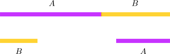 Figure 1
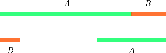 Figure 2
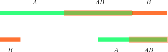 Figure 3
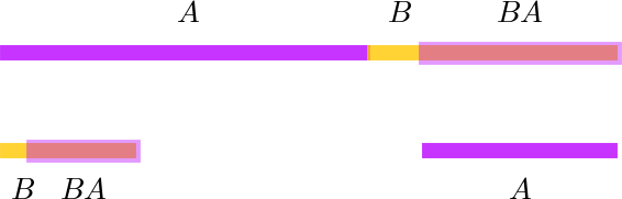 Figure 4
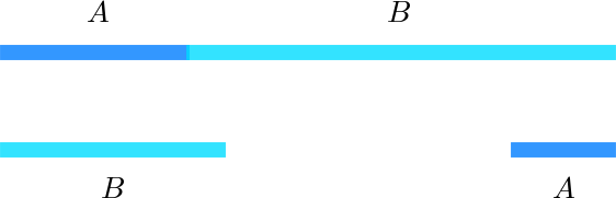 Figure 5
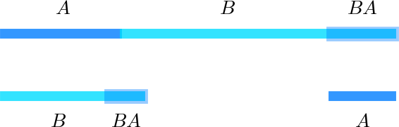 Figure 6
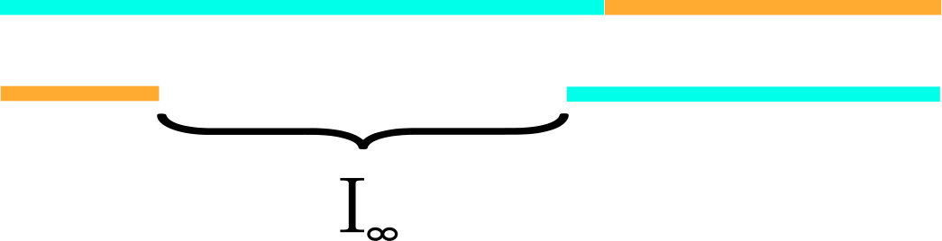 Figure 7
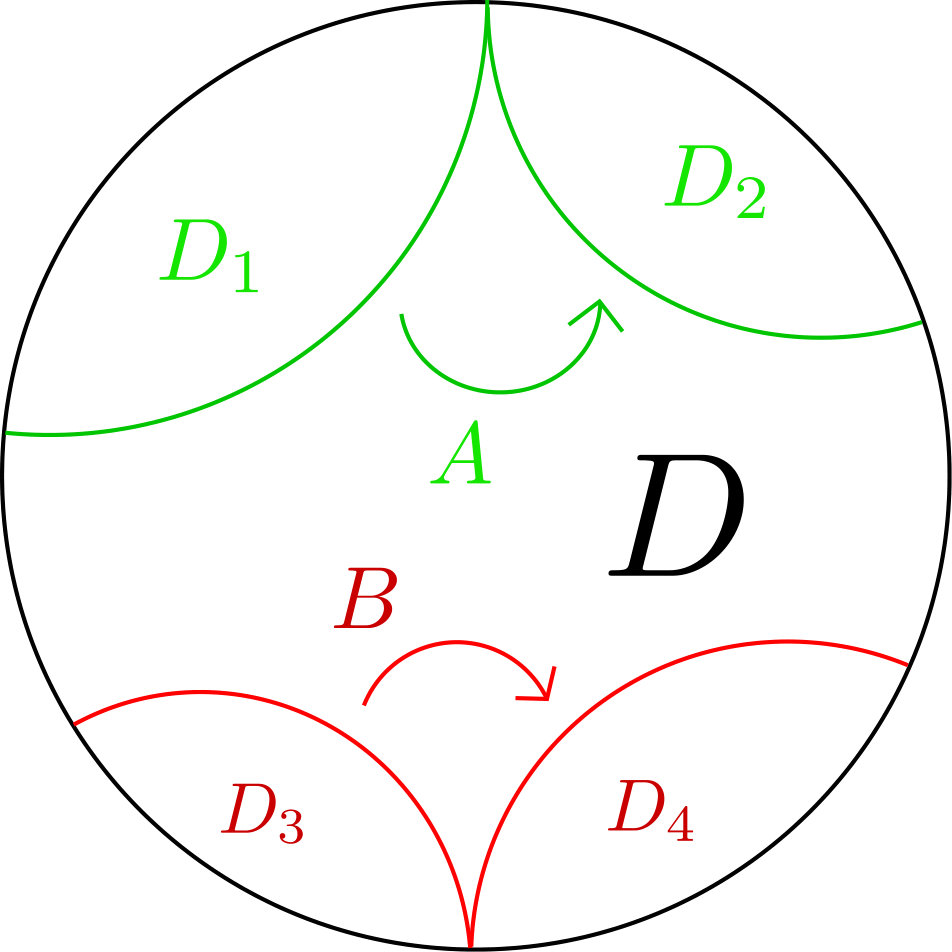 Figure 8
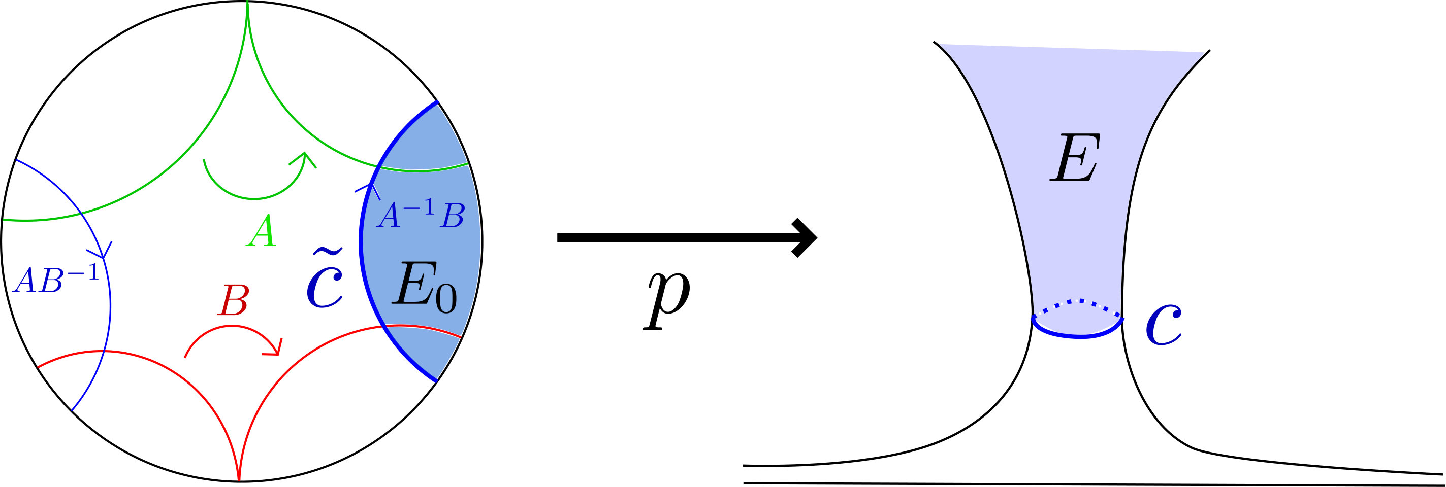 Figure 9
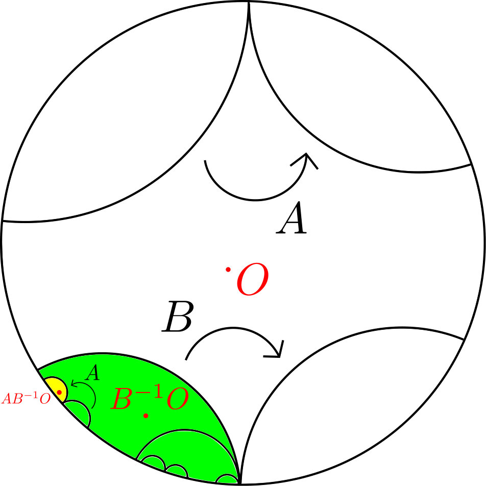 Figure 10
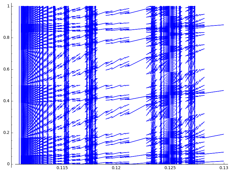 Figure 11
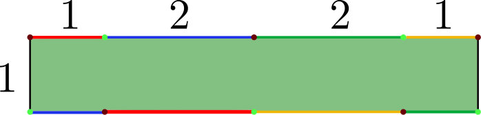 Figure 12
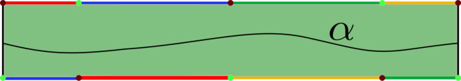 Figure 13
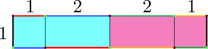 Figure 14
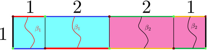 Figure 15
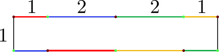 Figure 16
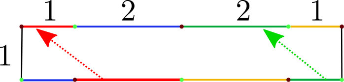 Figure 17
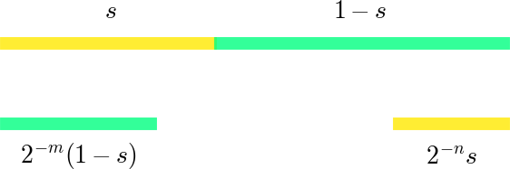 Figure 18
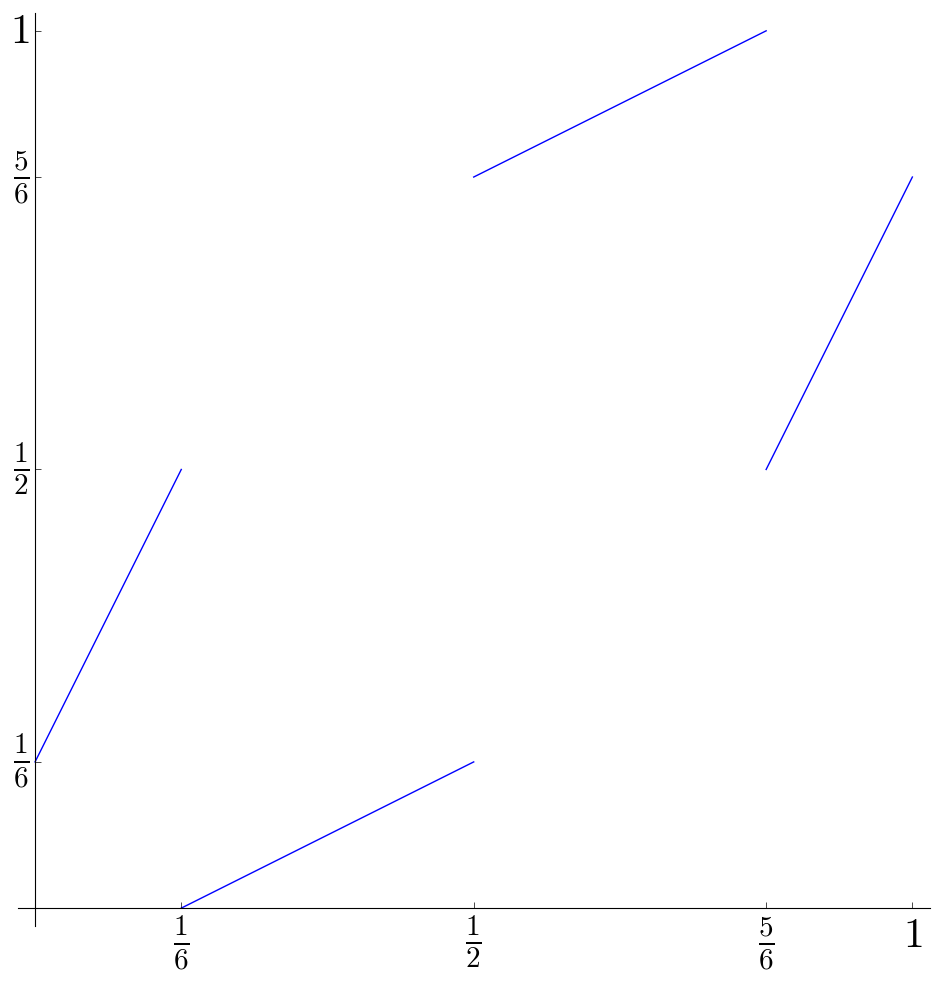 Figure 19
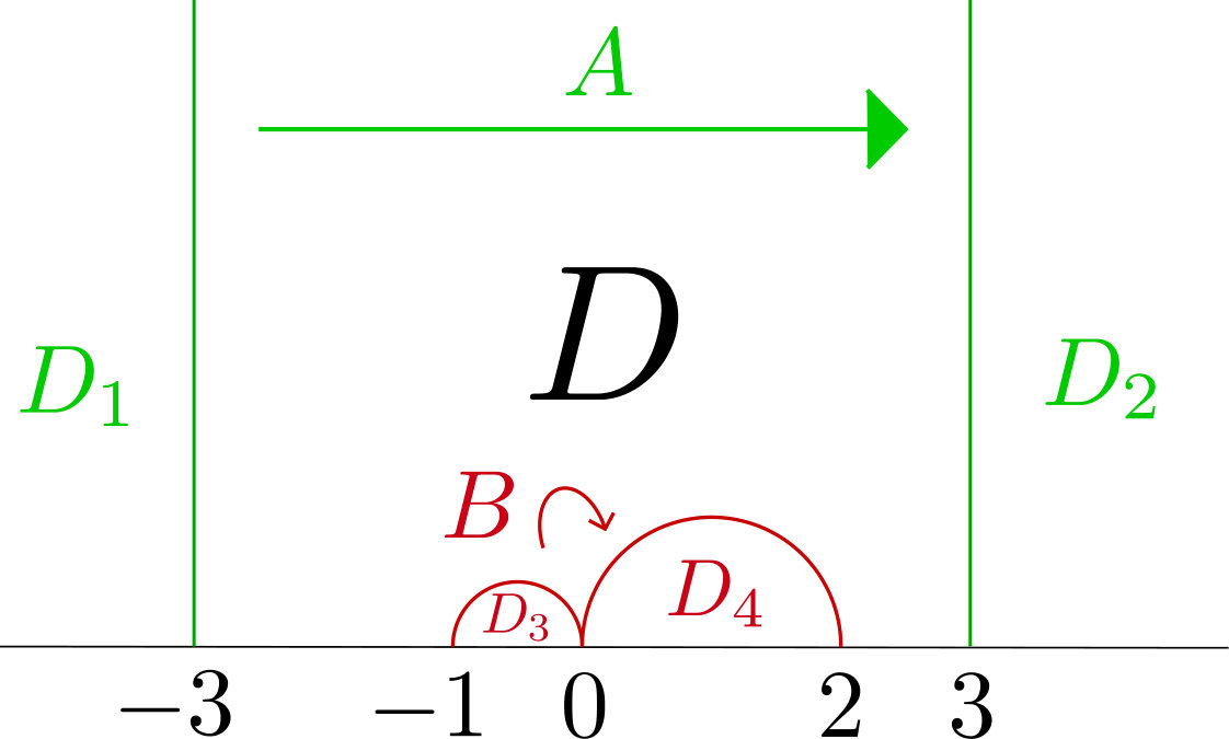 Figure 20
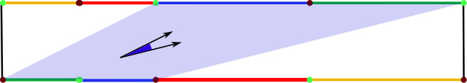 Figure 21
Peer Reviews
No public reviews on file for this paper yet. If you reviewed it on a platform where reviews are public (OpenReview, ICLR, NeurIPS, ICML), you can paste yours below so the community can read it here.
Videos
No videos yet. Explain this paper in a talk, walkthrough, or lecture? Add one.
Cascades in the dynamics of affine interval exchange transformations
Adrien Boulanger
,
Charles Fougeron
and
Selim Ghazouani
Abstract.
We describe in this article the dynamics of a -parameter family of affine interval exchange transformations. This amounts to studying the directional foliations of a particular dilatation surface introduced in [DFG], the Disco surface. We show that this family displays various dynamical behaviours: it is generically dynamically trivial but for a Cantor set of parameters the leaves of the foliations accumulate to a (transversely) Cantor set. This study is achieved through the analysis of the dynamics of the Veech group of this surface combined a modified version of Rauzy induction in the context of affine interval exchange transformations.
1. Introduction.
An affine interval exchange transformation (or AIET) is a piecewise continuous bijection of the interval which is affine restricted to its intervals of continuity. It has been known since the work of Levitt ([Lev82]) that AIETs can display as complicated a topological behaviour as dimension one allows: it can either be asymptotically periodic, minimal or (and this is the surprising part) have an invariant quasi-minimal Cantor set. In the latter case, the AIET would still be semi-conjugated to a minimal linear interval exchange transformation. In the spirit of generalising the theory of circle diffeomorphisms to piecewise continuous bijection of the interval, Camelier-Guttierez ([CG97]) begun a study of the regularity of the conjugacy between affine and linear IET, pursued by Cobo ([Cob02]), Bressaud-Hubert-Maas([BHM10]) and concluded by Marmi-Moussa-Yoccoz([MMY10]) who proved that almost every linear IET can be semi-conjugated to an AIET with an invariant Cantor set, in sharp contrast with Denjoy theorem in the case of sufficiently regular diffeomorphisms of the circle.
The goal of this article is to initiate a systematic study of the generic dynamical behaviour in parameter families of AIETs. The standard result in the theory of circle diffeomorphisms is a theorem by Herman (see [Her77]) predicting that for any (sufficiently regular) one-parameter family of circle diffeomorphisms, the set of minimal parameters has non-zero Lebesgue measure. On the other hand, it was known since the seminal work of Peixoto (see [Pei59], [Pei62]) that asymptotically periodic behaviour is topologically generic for flows on closed surfaces 111Generalised interval exchange transformations, of which AIETs are particular cases, should be thought of as first return maps of flows on higher genus surfaces, and a refinement of this theorem was proved by Liousse ([Lio95]) for transversally affine foliations in the case of higher genus surfaces. We present in this article a one parameter family of AIETs whose generic behaviour (in the measure theoretic sense) contrasts with the case of circle diffeomorphisms and Herman’s theorem.
We consider the map , where , defined the following way:
[TABLE]
The map is an affine interval exchange transformation (AIET) and one easily verifies that for all , . Its dynamical behaviour is therefore as simple as can be. Composing given maps by a family of linear rotations is a simple way to produce families of maps of the interval. Thus we consider the family , parametrised by S^{1}={\raisebox{1.99997pt}{\mathbb{R}}\left/\raisebox{-1.99997pt}{\mathbb{Z}}\right.} defined by
[TABLE]
where is the translation by modulo .
The following definition is of crucial importance for what follows. It was introduced by Liousse in [Lio95] who proved that this dynamical behaviour is topologically generic for transversally affine foliations on surfaces.
Recall that the orbit of a point under a map is the set and its -limit is the set of accumulation points of the sequence .
Definition 1**.**
We say that is dynamically trivial if there exists two periodic points of orders such that
- •
- •
- •
for all which is not in the orbit of , the -limit of is equal to the orbit of .
It means that the map has two periodic orbits, one of which attracting all the other orbits but the other periodic orbit which is repulsive. The following picture is the product of a numerical experiment representing periodic orbits in the family and their bifurcations.
This article aims at highlighting that this one-parameter family of AIETs displays rich and various dynamical behaviours. The analysis developed in it, using tools borrowed from the theory of geometric structures on surfaces, leads to the following theorems.
Theorem 2**.**
For Lebesgue-almost all , is dynamically trivial.
Our theorem is somewhat a strengthening of Liousse’s theorem for this -parameter family of AIETs and a counterexample to Herman’s in higher genus. Indeed, we prove that this genericity is also of measure theoretical nature. It is also worth pointing out that a lot of parameters in this family correspond to attracting exceptional minimal sets (i.e. which are homeomorphic to a Cantor set).
Theorem 3**.**
For all in a Cantor set of parameters in there exists a Cantor set such that for all , the -limit of is equal to .
The remaining parameters form a Cantor set denoted by . This notation is borrowed from Fuchsian group theory as we will indeed see that this Cantor set is the limit set of a subgroup . For parameters in , we have,
Theorem 4**.**
Let be the set of points in which are not fixed by a parabolic element of . Then
- •
for , the foliation is not dynamically trivial;
- •
for the foliation is totally periodic.
The foliations corresponding to directions in are also not totally periodic. Extensive computer experiments give evidences that these foliations are minimal.
Outline of the paper.
Sections 2 and 3 are devoted to recalling geometric basics about dilatation surfaces and to the study of the hidden symmetries of the family using this geometric perspective. Section 4 is mostly independent of the rest of the article. Therein we explain how to generalise the renormalisation procedure known as Rauzy-Veech induction to the context of piecewise contracting maps of the interval. This analysis allows the understanding of the dynamical behaviour of for sufficiently many parameters so that we can rely on the aforementioned symmetries to reach almost every parameter, which we explain in Section 6.
The discosurface
The first step of the proof consists in associating to the family a dilatation surface which we denote by obtained by the gluing represented in Picture 3.
As a dilatation surface is naturally endowed with a family of foliations which we call directional foliations. For definitions of both dilatation surfaces and these foliations we refer to Section 2.1. Our family of AIETs and these foliations are linked by the fact that the directional foliation in direction admits as their first return map on a cross-section, for . In particular they share the same dynamical properties hence the study of the family reduces to the study of the directional foliations of .
The Veech group of .
The major outcome of this change of point of view is the appearance of hidden symmetries. Indeed, the surface has non-trivial group of affine symmetries, i.e. a non-trivial group of diffeomorphisms given in charts as an element of the affine group of . All this material is defined in Section 2.2. Such a group of affine diffeomorphisms admits a natural representation in ; we call the image of this representation the Veech group that we denote by . This new group naturally acts on the set of directions of . The directions which are -equivalent through correspond to two foliations which are conjugated thus sharing the same dynamical behaviour. This remark will allow us to considerably reduce the number of parameters (equivalently ) that we need to analyse.
Using a standard construction of affine diffeomorphisms using flat cylinder decompositions recalled in Subsection 2.2.1, we show that the group is discrete and contains the following group
[TABLE]
The matrix belonging to it is natural to project to . We will hereafter make the slight abuse of notation to denote the image of by this projection as well. This group is a Schottky group of rank . The study of this action is performed in Section 3 and leads to the following.
- •
There is a Cantor set of measure zero on which acts minimally ( is the limit set of ).
- •
The action of on is properly discontinuous and the quotient is homeomorphic to a circle ( is the discontinuity set of ). It allows us to identify a "small" fundamental domain such that the description of the dynamics of foliations in directions implies the description for every parameter in (which is an open set of full measure).
Note that the Cantor set has nothing to do with the one described in Theorem 3. The latter is a subset of .
Affine Rauzy-Veech induction.
The study of the directional foliations for reduces to the understanding of the dynamics of piecewise contracting affine -intervals maps. To perform the dynamical study of these applications we adapt in this -contracting intervals setting a well known re-normalisation procedure, the Rauzy-Veech induction. The outcome of this method may be summarised as follows:
- •
there is a Cantor set of measure zero of parameters for which the associated foliation accumulates to a set which is locally a product of a Cantor set with an interval ;
- •
other directions in are dynamically trivial.
A remarkable corollary of the understanding of the dynamics of the directions in is the complete description of :
Theorem 5**.**
The Veech group of is exactly .
The proof is a rather straightforward corollary of the dynamical description. We prove that the limit set of is actually the same as the one of , and conclude using some elementary geometric arguments to prove that these groups are equal.
Acknowledgements.
We are grateful to Bertrand Deroin for his encouragements and the interest he has shown in our work. We are also very thankful to Pascal Hubert for having kindly answered the very many questions we asked him, to Vincent Delecroix, to Nicolas Tholozan for interesting discussions around the proof of Theorem 34 and to Matt Bainbridge.
2. Dilatation surfaces and their Veech groups.
We introduce in this section geometric objects which will play a role in this paper. This includes the definition of a dilatation surface, their associated foliations as well as their Veech groups, the construction of the Disco surface and how it is linked to our family of AIETs. We also compute explicitly two elements of the Veech group of the Disco surface.
2.1. Dilatation surfaces and their foliations.
Definition 6**.**
A dilatation surface is a surface together with a finite set and an atlas on whose charts take values in such that
- •
the transition maps are locally restriction of elements of ;
- •
each point of has a punctured neighbourhood which is affinely equivalent to the -sheets covering of .
We call an element of the set a singularity of the dilatation surface .
This definition is rather formal, and the picture one has to have in mind is that a dilatation surface is what one gets when you take a union of Euclidean polygons and glue together pairs of oriented parallel sides along the unique complex affine transformation that sends one to the other.
2.1.1. The Disco surface
The surface we are about to define will be the main object of interest of this text. It is the surface obtained after proceeding to the gluing below:
We call the resulting surface ’Disco’ surface. In the following will denote this particular surface. This is a genus dilatation surface which has two singular points of angle . They correspond to the vertices of the polygon drawn in Figure 5. Green (light) ones project onto one singular point and brown (dark) ones project onto the other.
2.1.2. Foliations and saddle connections.
Together with a dilatation surface comes a natural family of foliations. Fix an angle and consider the trivial foliation of by straight lines directed by . This foliation being invariant by the action of , it is well defined on and extends at points of to a singular foliation on such that its singular type at a point of is saddle-like. We denote this family of foliations by .
A saddle connection on is a singular leave that goes from a singular point to another. The set of saddle connections of a dilatation surface is countable hence so is the set of directions having saddle connections.
In the case of the Disco surface, one can easily draw these foliations on its polygonal model : they correspond to the restriction of the directional foliations of to the polygon. One can check that the horizontal curve on the picture below is actually a cross-section for every foliation with .
The first return map of the foliation with respect to this cross-section satisfies :
[TABLE]
2.2. The Veech group of a dilatation surface.
Let be a dilatation surface and an affine diffeomorphism of , namely a diffeomorphism which reads in dilatation coordinates as an element of the affine group of with the standard identification (more explicitly, a map of the form
[TABLE]
where and is a vector of ). We denote by the subgroup of of affine diffeomorphisms. The linear part in coordinates of an element of is well defined up to multiplication by a constant . This gives rise to a well-defined morphism:
[TABLE]
which to an affine diffeomorphism associates its normalised linear part. We call this morphism the Fuchsian representation.
Remark 7**.**
It is important to understand that the fact that the image of lies in is somewhat artificial and that the space it naturally lies in is . In particular, when an element of the Veech group is looked at in charts, there is no reason the determinant of its derivative should be equal to , however natural the charts are.
Definition 8**.**
The image of the Fuchsian representation is called the Veech group of and is denoted by . The Veech group naturally acts on the circle , we will refer hereafter to this action as the projective action of the Veech group.
The key point is that such an affine diffeomorphism maps the -directional foliation onto the foliation associated to the direction , in particular these two foliations are conjugated and therefore have the same dynamical behaviour. This allows us to reduce the amount of directional foliations to study to the set of parameters corresponding to the quotient of the circle by the projective action of the Veech group.
2.2.1. About the Veech group of .
This subsection is devoted to computing two elements of the Veech group. We utilise a method which is standard for translation surfaces, which consists in decomposing into flat cylinders of commensurable moduli and to let the multi-twist associated act affinely on each cylinder as a parabolic element.
Flat cylinders
A flat cylinder is the dilatation surface you get when gluing two opposite sides of a rectangle. The height of the cylinder is the length of the sides glued together and its width is the length of the non-glued sides, that is the boundary components of the resulting cylinder. Of course, only the ratio of these two quantities is actually a well-defined invariant of the flat cylinder, seen as a dilatation surface. More precisely, we define
[TABLE]
and call this quantity the modulus of the associated flat cylinder.
If is a cylinder of modulus , there is an element of which has the following properties:
- •
is the identity on ;
- •
acts as a unique Dehn twist of ;
- •
the matrix associated to is , if is assumed to be in the horizontal direction.
Decomposition in flat cylinders and parabolic elements
of the Veech group.
We say a dilatation surface has a decomposition in flat cylinders in a given direction(say the horizontal one) if there exists a finite number of saddle connections in this direction whose complement in is a union of flat cylinders. If additionally the flat cylinders have commensurable moduli, the Veech group of contains the matrix
[TABLE]
where is the smallest common multiple of all the moduli of the cylinders appearing in the cylinder decomposition. If the decomposition is in an another direction , the Veech group actually contains the conjugate of this matrix by a rotation of angle . Moreover, an affine diffeomorphism realising this matrix is a Dehn twist along the multi-curve made of all the simple closed curves associated to each of the cylinders of the decomposition.
Calculation of elements of the Veech group of
.
The above paragraph allows us to bring to light two parabolic elements in . Indeed, has two cylinder decompositions in the horizontal and vertical direction.
- •
The decomposition in the horizontal direction has one cylinder of modulus , represented Figure 6 below.
Applying the discussion of the last paragraph gives, we get that the matrix belongs to .
- •
The decomposition in the vertical direction has two cylinders, both of modulus , represented in Figure 7 below.
Again, we get that the matrix belongs to .
Finally notice that both the polygon and the gluing pattern we used to build is invariant by the rotation of angle , which implies that the matrix
[TABLE]
is realised by an involution in . Putting all the pieces together we get,
Proposition 9**.**
The group
[TABLE]
is a subgroup of .
3. The hyperbolic geometry of
3.1. The subgroup
We computed in Section 2 three elements , and of the Veech group of . The presence of the matrix in indicates that directional foliations on the surface are invariant by reversing orientation. This motivates the study of the Veech group action on \mathbb{RP}^{1}:={\raisebox{1.99997pt}{S^{1}}\left/\raisebox{-1.99997pt}{\mathrm{-Id}}\right.} instead of .
We will often identify to the interval by using projective coordinates:
[TABLE]
At the level of the Veech group it means projecting it to by the canonical projection . Let us denote by the group generated by the two elements:
[TABLE]
We will study the group as a Fuchsian group, that is a discrete group of isometries of the real hyperbolic plane . For the action of a Fuchsian group on , there are two invariant subsets which we will distinguish:
- •
one called its limit set on which acts minimally and that we will denote by ;
- •
the complement of which is called its discontinuity set, on which acts properly and discontinuously and which we will denote by .
We will give precise definitions in Section 3.3. In restriction to the discontinuity set, one can form the quotient by the action of the group. The topological space {\raisebox{1.99997pt}{\Omega_{\Phi}}\left/\raisebox{-1.99997pt}{\Phi}\right.} is a manifold of dimension one: a collection of real lines and circles.
We will show in Proposition 17 that for the group this set is a single circle, and therefore a fundamental domain for the action of the group can be taken to be a single interval (we will make it explicit: ). The dynamic of the directional foliations in the directions belonging to the interior of the interval will be studied in Section 4.
Remark 10**.**
We will prove in Section 6 that the group is actually equal to the full Veech group of the surface .
3.2. The action of the group on .
Two hyperbolic isometries are said to be in Schottky position if the following condition holds:
There exists four disjoints domains , which satisfy
[TABLE]
where denotes the complementary set of .
A group generated by two elements in Schottky position is also called a Schottky group. Figure 8 illustrates this situation.
Proposition 11**.**
The group is Schottky. Moreover the surface is a three punctured sphere with two cusps and one end of infinite volume.
Proof.
Viewed in the upper half plane model of the action is easily shown to be Schottky. In fact the action of (resp. ) becomes (resp. ). The two matrices are parabolic and fix and [math] respectively. Moreover, we observe that and . Figure 8 below shows that the two matrices and are in Schottky position with associated domains for .
The domain of Figure 8 is a fundamental domain for the action of . The isometry identifies the two green (light) boundaries of together and the two red (dark) ones. The quotient surface is homeomorphic to a three punctured sphere. ∎
3.3. The limit set and the discontinuity set.
The following notion will play a key role in our analysis of the affine dynamics of the surface :
Definition 12**.**
The limit set of a Fuchsian group is the set of accumulation points in of any orbit , where is the disk model for the hyperbolic plane .
The complementary set of the limit set is the good tool to understand the infinite volume part of such a surface.
Definition 13**.**
The complementary set is by definition the set of discontinuity of the action of on the circle.
The group acts properly and discontinuously on the set of discontinuity. One can thus form the quotient space {\raisebox{1.99997pt}{\Omega_{\Phi}}\left/\raisebox{-1.99997pt}{\Phi}\right.} which is a manifold of dimension one : a collection of circles and real lines. These sets are very well understood for Schottky groups thanks to the ping-pong Lemma, for further details and developments see [Dal11] chapter 4.
Proposition 14** (ping-pong lemma).**
A Schottky group is freely generated by any two elements in Schottky position. Moreover
- •
if the quotient surface {\raisebox{1.99997pt}{\mathbb{H}^{2}}\left/\raisebox{-1.99997pt}{\Phi}\right.} is of finite volume, the limit set is the full circle;
- •
otherwise, the limit set is homomorphic to a Cantor set.
Remark 15**.**
The third item case is the one of interest of this article.
The following theorem will be used in 6 to prove our main Theorem 2
Theorem 16** (Ahlfors, [Ahl66]).**
A finitely generated Fuchsian group satisfies the following alternative:
- (1)
either its limit set is the full circle ; 2. (2)
or its limit set is of zero Lebesgues measure
In our setting, it is clear that the limit set is not the full circle, thus the theorem implies that the limit set of is of zero Lebesgue measure.
3.4. The action on the discontinuity set and the fundamental
interval
The following proposition is the ultimate goal of this section.
Proposition 17**.**
The quotient space
[TABLE]
is a circle. A fundamental domain for the action of on corresponds to the interval of slopes .
Foliations defined by slopes which belong to this precise interval will be studied in section 4. To prove this proposition we will use the associated hyperbolic surface and link its geometrical and topological properties to the action of the group on the circle.
The definition of the limit set itself implies that it is invariant by the Fuchsian group. One can therefore seek a geometric interpretation of such a set on the quotient surface. We will consider the smallest convex set (for the hyperbolic metric) which contains all the geodesics which start and end in the limit set . We denote it by . Because the group is a group of isometries it preserves .
Definition 18**.**
The convex core of a hyperbolic surface , denoted by is defined as:
[TABLE]
As a quotient of a -invariant subset of , is a subset of the surface . The convex core of a Fuchsian group is a surface with geodesic boundary, moreover if the group is finitely generated the convex core has to be of finite volume. As a remark, a Fuchsian group is a lattice if and only if we have the equality . In the special case of the Schottky group the convex core is a surface whose boundary is a single closed geodesic as it is shown on Figure 9. For a finitely generated group we will see that we have a one to one correspondence between connected components of the boundary of the convex core and connected component of the quotient of the discontinuity set by the group.
The following lemma is the precise formulation of what we discussed above
Lemma 19**.**
Let a finitely generated Fuchsian group. Any connected component of the discontinuity set is stabilised by a cyclic group generated by a hyperbolic isometry . Moreover is composed of the two fixed points of the isometry .
We will keep notations introduced with Figure 9. We start by showing that for any choice of a lift in the universal cover of a geodesic in the boundary of the convex core one can associate an isometry verifying the properties of Lemma 19. Let be a closed geodesic consisting of a connected component of the boundary of the convex core of . One can choose a lift of such a geodesic in the universal cover, the geodesic is the axis of some hyperbolic isometry , whose fixed points are precisely the intersection of with the circle. As an element of the boundary of it cuts the surface into two pieces: and an end . One can check that this isometry is exactly the stabiliser of the connected component of whose boundary is the geodesic . Therefore such an isometry stabilises the connected component of the discontinuity set given by the endpoints of the geodesic . We have shown that given a boundary component of one can associate an element (in fact a conjugacy class) of the group which stabilises a connected component of . We will not show how to associate a geodesic in the boundary of the convex core to a connected component of the discontinuity set.
Remark 20**.**
We want to put the emphasis on the fact the assumption that the group is finitely generated will be used here. The key point is the geometric finiteness theorem [Kat92, Theorem 4.6.1] which asserts that any finitely generated group is also geometrically finite. It means that the action of such a group admits a polygonal fundamental domain with finitely many edges. It is not difficult to exhibit from such a fundamental domain the desired geodesic by looking at the pairing induced by the group, as it is done in Figure 9 for our Schottky group.
Corollary 21**.**
Connected components of {\raisebox{1.99997pt}{\Omega_{\Gamma}}\left/\raisebox{-1.99997pt}{\Gamma}\right.} are in one to one correspondence with infinite volume ends of the surface {\raisebox{1.99997pt}{\mathbb{H}^{2}}\left/\raisebox{-1.99997pt}{\Gamma}\right.}.
We now have all the material needed to prove Proposition 17.
Proof of Proposition 17.
Because the surface {\raisebox{1.99997pt}{\mathbb{H}^{2}}\left/\raisebox{-1.99997pt}{\Gamma}\right.} has only one end of infinite volume Corollary 21 gives immediately that {\raisebox{1.99997pt}{\Omega_{\Gamma}}\left/\raisebox{-1.99997pt}{\Gamma}\right.} is a single circle. Proof of the second part of Proposition 17 consists in a simple matrix computation. Figure 9 gives explicitly the elements of the group which stabilise a connected component of the discontinuity set. We then have to prove:
[TABLE]
where is the projective class of the vector . The computation is easy:
[TABLE]
∎
4. Generic directions and Rauzy induction.
The boundary of is canonically identified with through the natural embedding . Recall that the action of by Möbius transformations on is induced by matrix multiplication on after identification with by the dilatation chart . Thus the action of matrices of the Veech group on the set of directions corresponds to the action of these matrices as homographies on the boundary of .
We notice straight away that for directions with between and , there is an obvious attractive leaf of dilatation parameter (see Figure 10). There is also a repulsive closed leaf in this direction. This will always be the case since is in the Veech group, sending attractive closed leaves to repulsive closed leaves.
In the following we will describe dynamics of the directional foliation for between and . According to Section 2.2.1 the interval of direction is a fundamental domain for the action of on its discontinuity set. Moreover this discontinuity set has full Lebesgue measure in the set of directions thus understanding the dynamical behaviour of a typical direction therefore amounts to understanding it for . Further discussion on what happens in other directions will be done in the next section.
4.1. Reduction to an AI
The directions for have an appreciable property; they correspond to the directions of a subsurface invariant under the (oriented) foliation represented in Figure 11. Every leaf in the given angular set of directions that enters the subsurface will stay trapped in it thereafter. We therefore seek attractive closed leaves in this subset. To do so, take a horizontal interval joining the boundary components of this invariant subsurface and consider the first return map on it. It has a specific form (close to an affine interval exchange) which we will study in this section.
In the following, we use the notation AI to talk of a piecewise affine injection on an interval. For any , let be the set of AIs defined on with two intervals on which it is affine and such that the image of the left interval is an interval of its length divided by which rightmost point is , and that the image of its right interval is an interval of its length divided by which leftmost point is 0 (see Figure 12 for such an AI defined on ). When representing an AI, we will color the intervals on which it is affine in different colors, and represent a second interval on which we color the image of each interval with the corresponding color; this will be sufficient to characterise the map. The geometric representation motivates the fact that we call the former and latter sets of intervals the top and bottom intervals.
Note that the cross-sections defined on the subsurface of Figure 11 are in . We will study the dynamical behaviour of this family of AI.
4.2. Rauzy-Veech induction
Let be an AI and be its interval of definition. The first return map on a subinterval , is defined for every , as
[TABLE]
Since we have no information on the recurrence properties of an AI this first return map is a priori not defined on an arbitrary sub-interval. Nonetheless generalizing a wonderful algorithm of Rauzy [Rau79] for IETs, we get a family of subinterval on which this first return map is well defined. Associating to an AI its first return map on this well-chosen smaller interval will be called the Rauzy-Veech induction.
The general idea in the choice of this interval is to consider the smallest of the top and bottom intervals at one end of (left or right) the interval of definition. We then consider the first return map on minus this interval.
In the following we describe explicitly the induction for the simple family . A general and rigorous definition of Rauzy-Veech induction in the more general context of both AIs and AIETs is certainly possible with a lot of interesting questions emerging but is beyond the scope of this article.
Assume now that is an element of , let be the left and right top intervals of , and their length. Several distinct cases can happen,
-
(1)
-
(a)
i.e. .
We consider the first return map on . of length has no direct image by in but . Thus for the first return map, this interval will be sent directly to dividing its length by . We call this a right Rauzy-Veech induction of our AI. The new AI is in , and its length vector satisfies
[TABLE] 2. (b)
If i.e. .
In this case, the right Rauzy-Veech induction is not well-defined therefore we consider the first return map on which we call the left Rauzy-Veech induction of our AI. We obtain a new AI in and its length vector satisfies,
[TABLE]
Note that the two subcases presented above are mutually exclusive since the considered maps are strictly contracting. 2. (2)
i.e. and i.e. .
We consider the first return map on the subinterval . Then has no direct image by in but . Thus in the first return map, this interval will be sent directly to dividing its length by .
Then thus the induced map has an attractive fixed point of derivative .
Remark 22**.**
*The set of length for which we apply left or right Rauzy-Veech induction in the above trichotomy is exactly the set on which lengths and implied by the above formulas are both positive.
More precisely, 0\leq\lambda_{B}\leq 2^{-n}\lambda_{A}\iff R_{m,n}\cdot\left(\begin{array}[]{c}\lambda_{A}\\ \lambda_{B}\end{array}\right)\geq 0,
and 0\leq 2^{-m}\lambda_{B}\leq\lambda_{A}\iff L_{m,n}\cdot\left(\begin{array}[]{c}\lambda_{A}\\ \lambda_{B}\end{array}\right)\geq 0.
This will be useful later on to describe the set of parameters which corresponds to the sequence of induction moves we apply.
The algorithm.
We define in what follows an algorithm based on Rauzy induction that will allow us to determine if an element of has an attractive periodic orbit; and if so the length of its periodic orbit (or equivalently the dilatation coefficient of the associated leaf in ).
The algorithm goes the following way:
The entry is an element of ,
- (1)
If the entry is in case , perform in case the right Rauzy induction or in case the left Rauzy induction to obtain an element of or respectively. Repeat the loop with this new element. 2. (2)
If it is in case , it means that the first return map on a well chosen interval has a periodic attractive point of derivative . The algorithm stops.
Alongside the procedure comes a sequence of symbols and keeping track of whether we have performed the Rauzy induction on the left or on the right at the stage. This sequence is finite if and only if the algorithm described above finishes. An interesting phenomenon will happen for AI for which the induction never stops, and will be described latter.
4.3. Directions with attractive closed leaf
In the directions of Figure 11 corresponding to parameters in in projective coordinates, we consider the first return map of the directional foliation on the interval given by the two length 1 horizontal interval at the bottom of the rectangle. We have chosen directions such that the first return map is well defined although it is not bijective, and it belongs to . The ratio of the two top intervals’ length will vary smoothly between [math] and depending on the direction we choose. We parametrise this family of AI by , where is the length vector of the element of we get. The purpose of this section is to characterise the subspace for which the above algorithm stops, in particular they correspond to AI with a periodic orbit. The case of will be settled in the next subsection.
We describe for any finite word in the alphabet , , the subset of parameters for which the algorithm stops after the sequence of Rauzy-Veech induction moves.
We associate to the sequences , and defined by the recursive properties,
[TABLE]
[TABLE]
Let such that we can apply Rauzy-Veech inductions corresponding to to the element of of lengths . The induced AI after all the steps of the induction is in and its length vector is
[TABLE]
Following Remark 22, the property of being such that we can apply all the Rauzy-Veech inductions corresponding to to the initial AI in is equivalent to and . An induction on shows that it is an integer matrix with , , hence . will be the central subinterval of for which the induced AI in is in case .
Consider the sets
[TABLE]
Notice that has the same construction as the complement of the Cantor triadic set; each is constructed from by adding an interval in the interior of each interval which is a connected component of .
The rest of the subsection aims now at proving the following lemma,
Lemma 23**.**
* has full Lebesgue measure.*
As a preliminary we need the following Lemma which will be used later on in the proof.
Lemma 24**.**
For any word in , if M(w)=\left(\begin{array}[]{c c}a&b\\ c&d\\ \end{array}\right), we have,
[TABLE]
Proof.
The proof goes by induction on the length of . Let us assume that for some . We denote by
[TABLE]
Thus from which the inequality follows.
[TABLE]
The inequality is similar to the previous one. ∎
Proof of Lemma 23.
We will prove in the following that for any non-empty word ,
[TABLE]
for some . Thus at each step , is at least a -proportion larger in Lebesgue measure than . This implies the Lemma because
[TABLE]
We now show Inequality 25. Let be any finite word in the alphabet . For convenience we normalise the interval for such that it is . We denote by the length vector of the AI induced by the sequence of Rauzy-Veech inductions. These two lengths are linear functions of , is zero at the left end of the interval and is zero at the right end. As a consequence, these two functions have the form and for , where and are the maximal values of and respectively equal to according to the previous computations
[TABLE]
and
[TABLE]
We see that and similarly . Hence
[TABLE]
and
[TABLE]
thus
[TABLE]
If we denote by ,
[TABLE]
Lemma 24 implies directly that
[TABLE]
Hence for not empty, either or thus either
[TABLE]
∎
4.4. AI with infinite Rauzy-Veech induction
We focus in this subsection on what happens for AIs on which we apply Rauzy-Veech induction infinitely many times. First, remark that if we apply the induction on the same side infinitely many times, the length of the top interval of the corresponding side on the induced AI is multiplied each time by a positive power of , therefore it goes to infinity. Yet the total length of the subinterval is bounded by the length of the definition interval from which we started the induction. Thus the length of the interval has to be zero; this corresponds to the case where there is an attractive saddle connection, considered as a part of the cases treated above since we chose to take closed.
In consequence, for an AI with parameter in , we apply Rauzy-Veech induction infinitely many times, and the sequence of inductions we apply is not constant after a finite number of steps. Now let as above be the interval of definition of the given AI, and be its two intervals of continuity. Remark that the induction keeps the right end of and the left end of unchanged. Moreover the induction divides the length of one of the bottom interval (depending on which Rauzy-Veech induction we apply) by at least two because we iterate maps whose dilatation factor is at most . In turn if we consider to be the open subinterval of on which we consider the first return map after the -th induction, the limit of these nested intervals is
[TABLE]
By definition, this interval is disjoint from , and therefore
[TABLE]
Moreover, our definition of Rauzy-Veech induction implies that any point outside of the subinterval on which we consider the first return will end up in this subinterval in finite time. Thus
[TABLE]
Since we consider here only Rauzy-Veech induction procedure containing both infinitely right and left steps, we have that the orbit of any point of accumulates on .
Let be the complement of all the images of namely
[TABLE]
The measure of is , taking the image by divides the measure of any interval by two. Moreover, any two iterated images of this set are disjoint since is disjoint of the image set of the injective application , hence the measure of is . As we remarked, the orbit of any point of accumulates to and thus to any image of it, hence to any point of . As has full measure, has zero Lebesgue measure and thus has empty interior. To conclude, is the limit set of any orbit of .
Now is closed set with empty interior. Moreover, if we take a point in , any of its neighborhood contains some image of the interval since has zero measure, and thus its boundary. Hence no point is isolated, and is a Cantor set. Which leads to the following proposition,
Proposition 26**.**
In the space of directions there is a set (which is the union of the set constructed in this section union ) whose complement is a Cantor set of zero measure which satisfies
- •
* the foliation is attracted by an attracting leaf;*
- •
* is countable, and the foliation is attracted by a saddle connexion;*
- •
* is not countable, and the foliation concentrates on a stable Cantor set.*
5. Topological type of the elements of the Veech group
5.1. Thurston’s theorem on multi-twists.
We recall in this subsection a theorem of Thurston allowing the understanding of the topological type of the elements of a subgroup of generated by a couple of multi-twists. Let and be two multi-curve on . We say that
- •
and are tight if they intersect transversally and if their intersection number is minimal in their isotopy class;
- •
and fill up if is a union of cells.
Denote by and the components of and respectively. We form the matrix . One easily checks that is connected if and only if a power of is positive. Under this assumption, has a unique positive eigenvector of eigenvalue . We also denote by (resp. ) the Dehn twist along (resp. along ).
Theorem 27** (Theorem 7 of [Thu88]).**
Let and two multi-curves which are tight and which fill up , and assume that is connected. Denote by the subgroup of generated by and . There is a representation defined by
[TABLE]
such that is of finite order, reducible or pseudo-Anosov according to whether is elliptic, parabolic or pseudo-Anosov.
5.2. The case of .
We want to use Thurston’s theorem to prove the
Theorem 28**.**
For all , is of finite order, reducible or pseudo-Anosov according to whether its image by the Fuchsian representation in is elliptic, parabolic or hyperbolic.
In Subsection 2.2.1, we exhibited two elements of the Veech’s groupe , and as the images by the Fuchsian representation corresponding to the Dehn twists along the curves and drawn in Figure 16 :
One checks that:
- •
is connected;
- •
and are tight since they can both be realized as geodesics of ;
- •
and are filling up .
With an appropriate choice of orientation for and , we have that . The intersection matrix associated is therefore and . The parameter is then equal to and . We are left with two representations
[TABLE]
- (1)
is the restriction of the Fuchsian representation to composed with the projection onto . 2. (2)
is the representation given by Thurston’s theorem.
By definition of these two representations, maps to and maps it to ; and maps to and maps it to .
Proposition 29**.**
For all , and have same type.
Proof.
- •
and are faithful;
- •
and are Schottky subgroups of of infinite covolume;
- •
and send and to two parabolic elements;
As a consequence of these three facts, the quotient of by the respective actions of through and respectively are both a sphere with two cusps and a funnel. No element of or is elliptic, and the image of is parabolic in or if and only if the corresponding element in is in the free homotopy class of a simple closed curve circling a cusp. Which proves the proposition. ∎
There is little needed to complete the topological description of the elements of the Veech group of . Indeed, Proposition 29 above together with Thurston’s theorem ensures that the topological type of is determined by (the projection to of) its image by the Fuchsian representation (namely has finite order if is elliptic, is reducible if is parabolic and pseudo-Anosov if is hyperbolic).
The group has index in . The involution acting as preserves the multi-curves and and therefore commutes to the whole . In particular, any element of writes with . The type of is the same as the type of and this completes the classification.
6. The global picture.
Gathering all materials developed in the previous sections, we prove here the main theorems announced in the introduction.
Proposition 30**.**
Assume that the foliation of has a closed attracting leaf . Then it has a unique repulsing leaf and any leaf which is different from and regular accumulates on .
This proposition ensures that in all the cases where we have already found an attracting leaf, the dynamics of the foliation is as simple as can be.
Proof.
The proof consists in exhibiting the symmetry given by the element of the Veech group in this case. If the foliation given by the direction has an attractive hyperbolic leaf then, from the dynamical study performed in previous sections, one can suppose, up to applying an element of the Veech group, that such a direction lies in . Therefore, any point in the stable subsurface (see Figure 11) has to satisfy both the following:
- •
in positive time, the trajectory remains in the stable subsurface and is attracted to the closed leaf ;
- •
in negative time, it escapes the stable subsurface at some point.
The first item is basically what we proved in Subsection 4.3. The second one is proved by arguing on the -limit of a point , but for the foliation endowed with the reverse orientation. This set being invariant in both positive and negative time it has to be the closed leaf since it is the unique invariant set in the stable surface, see Subsection 4.3. This implies , which concludes.
Therefore, in negative time, the point must visit the other stable subsurface corresponding to the colors red and yellow of Figure 11, since the disco surface is the disjoint union of both these subsurfaces. This subsurface is stable for negative times, the point is therefore trapped in it. One can finally check that the dynamical study performed in Section 4.3 applies in the same way in this context, exchanging only the colors blue and green for red and yellow. In negative time, the point is then going to be attracted to the yellow red analogous leaf , which is repulsive if seen as a leaf of the oriented foliation. ∎
We say that a direction having such a dynamical behavior is dynamically trivial.
Corollary 31**.**
The directions in are not dynamically trivial.
Proof.
The set of directions fixed by a hyperbolic element of is dense in . Such a direction cannot be dynamically trivial, for otherwise the associated collection of closed leaves would be globally fixed by the corresponding element of , which can not occur since, according to Theorem 28, such an element is a pseudo-Anosov diffeomorphism. On the other hand, Proposition 30 shows that the set of dynamically trivial directions is the same as the set of directions admitting an attractive leaf, in particular both sets are open since the last one is. We conclude using the density in of the set of directions being not dynamically trivial: fixed points of hyperbolic matrices of . ∎
Theorem 32**.**
The set of dynamically trivial directions in is open and has full measure.
Proof.
Recall that the definition of and are given in Sections 2.2.1 and 3.1. Since belongs to the Veech group of , the foliations and have the same dynamical behaviour. We will therefore consider parameters in instead of in . We denote then by the set of dynamically trivial directions in . We have proved in Section 4 that the intersection of and is the complement of a Cantor set and that has full measure.
Also is a fundamental domain (see Proposition 11) for the action of on the discontinuity set of . Since , two directions in in the same orbit for the action of induce conjugated foliations on and therefore have same dynamical behaviour. This implies that is open and has full measure in . Since has itself full measure in , has full measure in . The fact that it is open is a consequence of the stability of dynamically trivial foliations for the topology, see [Lio95] for instance. ∎
Relying on a similar argument exploiting in a straightforward manner the action of the Veech group and the depiction of the dynamics made in Section 4, we get
Theorem 33**.**
There exists a Cantor set such that for all , the foliation accumulates to a set which is locally the product of a Cantor set with an interval. Such a set always have zero Lebesgue measure.
We believe it is worth pointing out that the method we used to find these ’Cantor like’ directions is essentially different compared to the one used in [CG97], [BHM10] and [MMY10]. Indeed they are proper attracting set in the sense that they have an open neighbourhood in which is pushed by the flow strictly within itself after a certain time.
These results allows us to give a complete description of .
Theorem 34**.**
The Veech group of is exactly .
Proof.
We divide the proof into four steps:
- (1)
proving that any element in preserves ; 2. (2)
proving that has finite index in ; 3. (3)
proving that the group is normal in ; 4. (4)
concluding.
(1) Let us prove the first point. Because of the description of the dynamics of the directional foliations we have achieved, one can show the limit set of the Veech group is the same as the limit set of . If not, there must be a point of in the fundamental interval . But since the group is non elementary it implies that we have to find in infinitely many copies of a fundamental domain for the action of on the discontinuity set. In particular infinitely many disjoint intervals corresponding to directions where the foliation has an attracting leaf of dilatation parameter . But by the study performed in the above section the only sub-interval of having this property is .
(2) The second point follows from the fact that the projection
[TABLE]
induces an isometric orbifold covering
[TABLE]
Since has finite volume (see Section 3.2) and because
[TABLE]
, this ratio must be finite and hence has finite index in .
(3) Remark that is generated by two parabolic elements and and that these define the only two conjugacy class in of parabolic elements. We are going to prove that any element normalise both and . Since has finite index in , there exists such that . There are but two classes of conjugacy of parabolic elements in which are the ones of and . If , this implies that contains a strict divisor of , which would make the limit set of larger that (consider the eigenvalues of the matrix which determine points in the boundary on the limit set, see Lemma 19). Therefore belongs to . A similar argument shows that and since and generate , normalises . Hence is normal in .
(4) Any thus acts on the convex core of the surface . In particular it has to preserve the boundary of , which is a single geodesic by Proposition 17. At the universal cover it means that has to fix a lift of the geodesic , thus the isometry permutes two fixed points of a hyperbolic element of . Two situations can occur:
- •
is an elliptic element. His action on cannot permute the two cusps because they correspond to two essentially different cylinder decompositions on . It therefore fixes the two cusps and hence must be trivial.
- •
is hyperbolic and fixes the two fixed points of . Moreover, by Lemma 19, it acts on the fundamental interval and as we discussed above such an action has to be trivial because of our study of the associated directional foliations, the translation length of is then the same than . But is fully determined by its fixed points and its translation length, which shows that and thus .
Any element of therefore belongs to and the theorem is proven. ∎
Remark 35**.**
This theorem implies that the completely periodic directions correspond to the orbit by the Veech group of the horizontal and vertical directions, since any parabolic element is conjugated to the Dehn twist in one of these two directions. This is the set we denoted by in Theorem 4.
The reference list from the paper itself. Each links out to its DOI / PubMed record.
- 1[Ahl 66] Lars V. Ahlfors. Fundamental polyhedrons and limit point sets of Kleinian groups. Proc. Nat. Acad. Sci. U.S.A. , 55:251–254, 1966.
- 2[BHM 10] Xavier Bressaud, Pascal Hubert, and Alejandro Maass. Persistence of wandering intervals in self-similar affine interval exchange transformations. Ergodic Theory Dynam. Systems , 30(3):665–686, 2010.
- 3[CG 97] Ricardo Camelier and Carlos Gutierrez. Affine interval exchange transformations with wandering intervals. Ergodic Theory Dynam. Systems , 17(6):1315–1338, 1997.
- 4[Cob 02] Milton Cobo. Piece-wise affine maps conjugate to interval exchanges. Ergodic Theory Dynam. Systems , 22(2):375–407, 2002.
- 5[Dal 11] Francoise Dal’Bo. Geodesic and horocyclic trajectories . Universitext. Springer-Verlag London, 1 edition, 2011.
- 6[DFG] Eduard Duryev, Carlos Fougeroc, and Selim Ghazouani. Affine surfaces and their veech groups. ar Xiv preprint , https://arxiv.org/abs/1609.02130.
- 7[Her 77] Michael-Robert Herman. Mesure de Lebesgue et nombre de rotation. pages 271–293. Lecture Notes in Math., Vol 597, 1977.
- 8[Kat 92] Svetlana Katok. Fuchsian groups . Chicago lectures in mathematics series. University of Chicago Press, 1 edition, 1992.