A Quick View of Lagrangian Floer Homology
Andr\'es Pedroza

TL;DR
This paper provides an accessible overview of Lagrangian Floer homology, its foundational concepts in symplectic geometry, and its role in addressing Arnol'd's conjecture on fixed points of Hamiltonian diffeomorphisms.
Contribution
It offers a concise introduction connecting Floer homology with symplectic geometry and the Arnol'd conjecture, highlighting key ideas and their interrelations.
Findings
Explains the basics of Morse theory and critical points.
Introduces symplectic geometry concepts relevant to Floer homology.
Describes the connection between Floer homology and Arnol'd's conjecture.
Abstract
In this note we present a brief introduction to Lagrangian Floer homology and its relation with the solution of Arnol'd conjecture, on the minimal number of non-degenerate fixed points of a Hamiltonian diffeomorphism. We start with the basic definition of critical point on smooth manifolds, in oder to sketch some aspects of Morse theory. Introduction to the basics concepts of symplectic geometry are also included, with the idea of understanding the statement of Arnol'd Conjecture and how is related to the intersection of Lagrangian submanifolds.
Click any figure to enlarge with its caption.
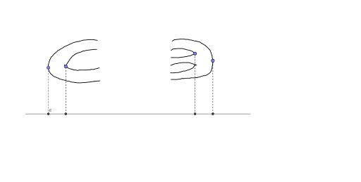 Figure 1
Peer Reviews
No public reviews on file for this paper yet. If you reviewed it on a platform where reviews are public (OpenReview, ICLR, NeurIPS, ICML), you can paste yours below so the community can read it here.
Videos
No videos yet. Explain this paper in a talk, walkthrough, or lecture? Add one.
Taxonomy
TopicsGeometric and Algebraic Topology · Topological and Geometric Data Analysis · Mathematical Dynamics and Fractals
11institutetext: Andrés Pedroza 22institutetext: Facultad de Ciencias, Universidad de Colima, Bernal Díaz del Castillo No. 340, Colima, Col., Mexico 28045 22email: [email protected]
A Quick View of Lagrangian Floer Homology
Andrés Pedroza
Abstract
In this note we present a brief introduction to Lagrangian Floer homology and its relation with the solution of Arnol’d conjecture, on the minimal number of non-degenerate fixed points of a Hamiltonian diffeomorphism. We start with the basic definition of critical point on smooth manifolds, in oder to sketch some aspects of Morse theory. Introduction to the basics concepts of symplectic geometry are also included, with the idea of understanding the statement of Arnol’d Conjecture and how is related to the intersection of Lagrangian submanifolds.
1 Introduction
Many elegant results in mathematics have to deal with the fixed-point-set of a function. For example: Brouwer fixed-point theorem, Lefschetz fixed-point theorem, Banach fixed-point theorem and Poincaré-Birkhoff theorem, just to name a few. Furthermore, these results are fundamental in their own area of mathematics and have interesting consequences in diverse areas of mathematics; differential equations, topology and game theory among others. Symplectic geometry has its own fixed-point theorem, which was conjectured by V. Arnol’d arnold-sur in 1965. The Arnol’d Conjecture was motivated by Poincaré-Birkhoff theorem: An area-preserving diffeomorphism of the annulus which maps the boundary circles to themselves in different direction, must have at least two fixed points.
The generalization of Poincaré-Birkhoff theorem fits in symplectic geometry and not in volume-preserving geometry. The Arnol’d Conjecture establishes a lower bound on the number of fixed points a Hamiltonian diffeomorphism in terms of the topology of the manifold. The fixed points of a Hamiltonian diffeomorphism, (in fact any diffeomorphisms) can be seen as the intersection of its graph and the diagonal. In the context of symplectic geometry, is the intersection of two Lagrangian submanifolds.
In 1987, A. Floer floer-morse developed a homological theory that focused on the intersection of Lagrangian submanifolds. In particular, under some hypotheses, he proved the Arnol’d Conjecture for a particular class of closed symplectic manifolds. This theory is called Lagrangian Floer homology.
In these notes we sketch how Lagrangian Floer homology is defined. In fact we review some aspects of Morse theory from its basics; like non-degenerate critical points, the Hessian, flow lines of the gradient vector field up to Morse homology. The reason being, that Lagrangian Floer homology emulates in many aspects Morse homology. Also we cover the basics of symplectic manifolds and Hamiltonian diffeomorphisms. The last section deals with Lagrangian Floer homology and how it is used to prove the Arnol’d Conjecture.
For the basic notions of differential geometry the reader can look at tu-man ; for the aspects of symplectic geometry cannas-lectures and ms ; and also msjholo where the analytical aspect of holomorphic curves is covered. For details and proofs on the construction of Lagrangian Floer homology see audin-morseth , oh-symplectic1 and oh-symplectic2 . For an excellent introduction to Fukaya categories see aauroux-a ; and seidel-fukcat for a detail treatment of the subject.
These lecture notes are based on a course given at the 7th. Mini Meeting on Differential Geometry held at CIMAT in February 2015. The author wishes thank the organizers and participants for the pleasent atmospere. Finally the author was partially supported by a CONACYT grant CB-2010/151846.
2 Morse-Smale Functions
Let be a smooth manifold of dimension and a smooth function. A point is called a critical point of if the differential at is the zero map. Denote by the set of critical points of . Notice that can be the empty set, however if is compact then it is not empty, since a smooth function on has a maximum and a minimum.
Let be a critical point of and a coordinate chart about . The Hessian matrix of at relative to the chart , is the matrix
[TABLE]
A critical point is said to be non-degenerate if the matrix is non-singular. Note that the Hessian matrix is symmetric, hence if it is non-singular its eigenvalues are real and non-zero. The index of at a non-degenerate critical point , which is denoted by , is defined as the number of negative eigenvalues of the Hessian matrix at .
The definition of the index at a non-degenerate critical point given above depends on the coordinate system; however it can be shown that the is independent of the coordinate system about the the critical point.There is an alternative definition of the index of a function at a non-degenerate critical point, that does not needs a coordinate system. For a critical point of define the bilinear form
[TABLE]
as , where is any vector field on whose value at is . Notice that since is a critical point of , the bilinear form is symmetric,
[TABLE]
In this context, is called non-degenerate if the bilinear symmetric form is non-degenerate. The index of at is defined as the number of negative eigenvalues of the symmetric bilinear form . The two definitions given of non-degenerate critical point agree. The same applies for the two definitions of the index of a non-degenerate critical point. For further details, see (audin-morseth, , Ch. 1) and liviu-morse .
Definition 1
A smooth function for which all of its critical points are non-degenerate is called a Morse function.
Now we consider some examples in the case when . The origin is the only critical point of the function . Moreover is a non-degenerate critical point and its index is zero. The origin is also the only non-degenerate critical point of the functions and . In these cases the index at the origin is 1 and 2 respectively. These three examples describe the general behavior of a function on near the origin when it is a non-degenerate critical point. The precise statement on the behavior of a function near a non-degenerate critical point is given by Morse lemma.
Theorem 2.1 (Morse Lemma)
Let be a smooth function such that the origin is a non-degenerate critical point of index . Then there exists a coordinate chart about the origin such that
[TABLE]
It goes without saying that Morse lemma also holds for smooth functions defined on arbitrary manifolds. A consequence of Morse lemma, as stated above, is that there exists a neighborhood about the origin in so that it is the only critical point in such neighborhood.
Corollary 1
Non-degenerate critical points of a smooth function are isolated.
Note that a Morse function defined on a compact manifold has finitely many critical points.
The main reason behind the study of Morse functions is to understand the topology of the manifold. Thus for a smooth function and define the level set
[TABLE]
Notice that when is the absolute minimum of , then is empty for every . And in the case when is the absolute maximum of , then for every .
Now we explain what we mean by understanding the topology of the manifold; one aspect is that the manifold can be constructed from information from a fixed Morse function on it. Consider a compact manifold , a smooth Morse function and for simplicity assume that are all the critical points, with and for . Thus achieves its minimum at and ; and it achieves its maximum at and . In order to build the manifold from the critical points of , one starts with the point . Then from Theorem 2.2 below, it follows that has the same homotopy type has for . By an -cell we mean a space homeomorphic to the closed ball of dimension . Hence, is homeomorphic to the -cell for .
The next step is to analyze the next non-degenerte critical point . In this case for , it follows that has the same homotopy type as with a -cell attached. That is , where is a gluing function. This process continues at every critical point. That is for the space as the same homotopy type has to with an attached -cell. The last step asserts that for ; that is is homeomorphic to minus an open ball. Therefore is homeomorphic to with a -ball attached. Note that the change of topology between the level sets occurs precisely at the critical points of Below, we carry out the same process described above for
Therefore when is a Morse function, is possible to describe the topology of the level sets as increases; in particular the topology of . Furthermore, there is an alternative approach to understand the topology of using a Morse function. This is called Morse homology and it will be describe in Section 3.
Theorem 2.2
Let be a Morse function.
- •
If has no critical value in , then is diffeomorphic to .
- •
If has only one critical value in of index , then has the same homotopy type as that of , for some gluing function .
As above, means that is attached to by some gluing function . Note that is diffeomorphic to . In the next example, we show how Theorem 2.2 is used to obtain the whole manifold , by attaching one -cell at a time.
Example 1
Consider the real projective space , the set of lines through the origin in . A point in is represented in homogeneous coordinates as . Let be distinct real numbers, define by
[TABLE]
So defined is smooth and since the are distinct it has non-degenerate critical points, that are . Thus is a Morse function; moreover the critical point has index .
The reader is encouraged to verify the statements made above. And also to get the same conclusions for the case of the complex projective space with the function
[TABLE]
Now we look at the particular case of ; recall that is diffeomorphic to the circle. In this particular case take and , so takes the form
[TABLE]
In this case has only one critical point of index [math], namely at . It also has only one critical point of index , at . These points correspond to the maximum and minimum of . In terms of Theorem 2.2 the circle is obtained as follows. We start with the [math]-cell that is just a point, that is . Since has no critical values in the interval other than [math], then from Theorem 2.2 if follows that has the same homotopy type has . Notice that is a semicircle, the south hemisphere. Next comes the other critical point . It has index ; thus a -cell is attached to . That is, the two points of get glued to to obtain the circle. See Figure 1.
An important aspect to consider is the existence of Morse functions on a given manifold. It turns out that there are plenty of Morse functions. More precisely, the set of Morse functions on a closed manifold is -dense in the space of smooth functions. The reason that the -topology is needed is because the concept of non-degenerate critical points involves derivatives up to second-order. In theory, is not to difficult to understand the topology of via a Morse function as above. Next we take this idea a step further to recover the homology of .
Fix a Riemannian metric on and let be the induced inner product on its tangent bundle. The gradient vector field, , of the function is defined by the equation
[TABLE]
for every vector field on . Notice that if is a critical point of , then . And conversely, if then is a critical point of Therefore equals the zero set of .
In order to simplify the exposition, from now on we assume that is compact. Denote by the flow of the negative gradient vector field of . Thus for
[TABLE]
The reason to consider the negative gradient vector field is only a matter of convention. Note that and if is a non-degenerate critical point of , then where is the dimension of . Also notice that outside the set of critical points of , hence points in the direction in which is decreasing. The way to think about the index of a non-degenerate critical point is the number of linearly independent directions in which the decreases. Let be a point where vanishes, then consider all points of that under the flow converge to as goes to infinity;
[TABLE]
Similarly,
[TABLE]
the set of all points in that have has a source. Since vanishes at , then the critical point is a fixed under the flow, hence and . The submanifolds and are called the unstable manifold and stable submanifold of at , respectively.
Theorem 2.3
If is a non-degenerate critical point of , then is a smooth submanifold of of dimension .
Instead, if we consider the function the set critical non-degenerate points of and agree. Moreover and . Hence is also a smooth submanifold of of dimension .
Example 2
Let be the unit sphere in centered at the origin and defined as . Then the poles and are the critical points of . Furthermore they are non-degenerate, has index 2 and has index 0.
Consider the Riemannian structure on induced from the standard Riemannian structure on . Then is the vector field that points downwards, and
[TABLE]
Example 3
Consider the function given by
[TABLE]
So defined induces a smooth function on the flat two-dimensional torus , which we still denote by . There are non-degenerate critical points on the torus, and of index and [math] respectively. Consider the Riemannian structure on induced from the canonical Riemannian structure on . Then the flow of can be seen in Figure 3.
Notice that there are only two lines that connect to . And a 1-dimensional family of flow lines that connect to , whose points determine four open connected components of the torus.
Also Figure 3 gives a description of the stable and unstable submanifolds. Observe that every interior point of , lies in a flow line that ends at . That is,
[TABLE]
Similarly we have that equals
[TABLE]
and
[TABLE]
Let and be non-degenerate critical points of a smooth function . Then the set consists of points of that belong to a flow line of that connects to ; that is
[TABLE]
We know from Theorem 2.3 that and are submanifolds of , but their intersection might not be a smooth manifold. Hence a smooth function is said to satisfy the Smale condition if for any pair of critical points and , and intersect transversally. In particular is a submanifold of .
The function that appears in Example 2 satisfies the Smale condition. In this example the intersection of any pair of stable and unstable submanifolds is either empty, a point, the sphere minus a point or the sphere minus two points. Also the Moorse function in Example 3 satisfies the Smale condition. In particular, notice that consists of two disjoint open intervals.
The type of functions that are of interest in this note are the Morse-Smale functions. For an arbitrary compact manifold and Riemannian metric, there always exists a Morse-Smale function. Furthermore, in some sense there are plenty of such functions. Then if is a Riemannian manifold and a Morse-Smale function we write for the set of points of that belong to a flow trajectory of that goes from to as in Eq. (1). Notice that in this case is a smooth submanifold of of dimension . Note that the submanifold admits a natural action of defined as for . The action is in fact free and the orbit space of this action is denoted by . Hence is identified as the space of trajectories that joint to
So defined, the space of points that belong to a flow line of that connect to , , is not necessarily compact. For example, in the case of the two-spere in Example 2 we have that is . In this example if we add the critical points we obtain a compact space, namely the whole manifold . Note that in this example is diffeomorphic to But it is not always the case that by adding the critical points and to that it becomes a compact space. For instance, in the torus case of Example 3 the space is not compact.
In general, the way to compactify the space of trajectories is by adding broken trajectories. A broken trajectory from to is a collection of flow lines of such that connects the critical points to for where and Consider the bigger set of flow lines that connect to , namely usal flow trajectories plus broken trajectories,
[TABLE]
Recall that the index of critical points of decreases along flow lines. Hence the number of flow lines that form a broken flow lines is less than . Hence if there are no broken trajectories connecting to and . That is, is compact in this case and it consists of finitely many points.
The proof of the next result can consulted in (audin-morseth, , Chp. 3) and salamon-lectures .
Proposition 1
Let be a closed Riemannian manifold, a Morse-Smale function and critical points of . Then the natural action of on is free. Moreover is smooth and compact of dimension
The important case that would be relevant later on is the case when . Usually in this case the space is not compact, so we must add broken trajectories. Hence is a finite collection of closed intervals and circles.
In Example 3 consider and , for two flow lines of . The flow line connects to , and connects to . Hence is a broken trajectory that connects to . Note that is diffeomorphic to four copies of ; and there are eight broken trajectories that must be added to obtain . For instance, is one of them. Henceforth is diffeomorphic to four copies of
3 Morse Homology
We are going to define the Morse-Witten complex of ; the Riemannian manifold and the Morse-Smale function. For simplicity we will use coefficients, keep in mind that it is possible to use integer coefficients. In order to define Morse homology with integer coefficients, one must prove that is possible to have a coherent system of orientation on the compact moduli spaces. In the case of coefficients the orientation of the moduli spaces is irrelevant, only the boundary components of the moduli spaces of dimension two are important. See for example salamon-lectures , where they use integer coefficients. Also we drop the dependence of the Riemannian metric from the notation. Denote by the set of critical points of index and by the -vector space generated by the elements of . For , define to be the trivial vector space. If and are critical points of such that , then by Proposition 1 is a finite set of points. Denote by the number of points of module 2.
The boundary operator, , is the linear map defined on generators as
[TABLE]
Notice that if is zero-dimensional, then consists of finitely many lines that connect to . This geometric description of is useful when computing the boundary operator ; this will be seen for instance below in Example 4. The reason why is called the boundary operator is given by the next result.
In order to compute one must consider the moduli spaces where For ,
[TABLE]
where stands for the number of points of . Notice that is a one-dimensional compact manifold; hence it is the union of a finite collection of closed intervals and circles. Hence its boundary consists of a even number of points which are
[TABLE]
and correspond to the broken trajectories from to that go thru .
Theorem 3.1
The operator satisfies .
The complex is called the Morse-Witten complex of . Its homology
[TABLE]
is called the Morse homology of with -coefficients. Note that the relevant moduli spaces for the definition of Morse homology are those whose dimension is at most two.
Remark 1
As mention above is possible to define Morse homology with coefficients. For, is an orientable submanifold of for any critical point . Hence, one fixes an orientation on for every critical point. This yields an orientation on and hence on and . Thus if , then is a finite set of points each of which has a sign. Set to be the sum of these signs; then the boundary operator over -coefficients is defined as
[TABLE]
However the statement is delicate in this case. One must take into consideration that the orientation of the moduli spaces of dimension two induced the right orientation on its boundary; the one-dimensional moduli spaces. For example see salamon-lectures .
Recall from Example 2, that on we defined a Morse function with the poles and as critical points of index 2 and 0 respectively. The Riemannian structure on the sphere was induced from the canonical Riemannian structure on . Further, we calculated the stable and unstable submanifolds of and . From this calculation, it follows that is a Morse-Smale function. Therefore , and the boundary operator is the zero map. Hence
[TABLE]
Example 4
In this example we consider the function on the two-dimensional torus defined in Example 3. Notice that the function is Morse-Smale. Hence and . Counting trajectory flow lines, we get , , , and . Therefore,
[TABLE]
Summing up, we started with a smooth closed manifold , then we choose a smooth function and a Riemannian metric , such that the critical points of were non-degenerate and the intersection of the stable and unstable submanifolds were transversal. With all these data, we defined the Morse homology of At the end, Morse homology is a topological invariant of the manifold; that is, is independent of the function and the Riemannian metric. Furthermore it recovers the ordinary homology of the manifold. See schwarz-mor and witten-super .
Theorem 3.2
Let be a compact manifold, a Riemannian metric and a Morse-Smale function. Then is independent of the function and the metric. Moreover as vectors spaces for every .
In the words of R. Bott bott-morse , Morse theory indomitable. Here we barely treated the subject and its consequences. The reader is encouraged to learn more about the subject in bott-morse , matsumoto-morse , liviu-morse and in the beautiful monograph of J. Milnor, milnor-morse . One application of Morse theory is the handlebody decomposition of a manifold; a much finer result than that stated in Theorem 3.2. In particular the Bott periodicity theorem is a marvelous consequence of Morse theory. Another typical consequence of Morse theory are the Morse inequalities. Here the problem is to determine lower bounds for the number of critical points of a fixed index of a Morse function. Denote by the -Betti number of , that is the rank of .
Theorem 3.3 (Morse’s inequalities)
Let be a a closed manifold and a Morse function. Then
[TABLE]
for every .
Thus Morse theory gives a lower bound for the minimal number of critical points that a Morse function can have on a manifold. Finally we mention that some features of ordinary homology, for example Poincaré duality and product operations, can be described in the Morse homology setting. See fukaya-morsehomotopy , schwarz-mor and witten-super .
4 Symplectic Manifolds and Lagrangian Submanifolds
A symplectic form on a manifold is -form that is closed and non-degenerate. Here non-degenerate means that at every and every nonzero vector there exists a vector such that is nonzero. In this case is called a symplectic manifold. The symplectic form been non-degenerate, implies that the dimension of must be even. Unless otherwise stated from now on we assume that the dimension of is .
The first and fundamental example of a symplectic manifold is . Here we take as coordinates in and the symplectic form is defined as
[TABLE]
In the 2-dimensional case, a symplectic form is the same as a volume form. Hence an oriented surface together with a volume form is an example of a symplectic manifold.
Example 5
Let be the unit sphere in centered at the origin. Then for and define
[TABLE]
where is the inner product and is the cross product in . So defined is a non-degenerate -form on the sphere. By dimension reasons, ; therefore is a symplectic form on the unit 2-sphere.
Example 6
Another important class of examples of symplectic manifolds are cotangent bundles of any smooth manifold . Let be the projection map and its differential at . Define the 1-form on at as
[TABLE]
Then the canonical symplectic form on is defined as . This example is particularly important in Classical Mechanics. In fact the roots of symplectic geometry go back to Classical Mechanics. For example see arnold-math .
In particular if with coordinates and the fibre with coordinates , then has coordinates . In this case the 1-form defined above takes the form
[TABLE]
Moreover ; hence on we get the symplectic form defined at the beginning of this section.
Another source of examples of symplectic manifolds are Kähler manifolds. In particular the complex projective space admits a symplectic form called the Fubini-Study symplectic form, which is induced from the Fubini-Study hermitian metric. That is, if is a canonical open set, then on the Fubini-Study symplectic form is defined as
[TABLE]
Furthermore, the symplectic area of the complex line is .
It is also possible to create new symplectic manifolds from old ones. Cartesian product of symplectic manifolds is such an example; since this example will be of importance later on we explain it in Example 7. Nonetheless there are more ways to create new symplectic manifolds, such as: symplectic reduction, fibrations and blow ups just to name a few.
Example 7
Let and a symplectic manifolds and consider with projection maps and . Then is a symplectic manifold. In particular for the same symplectic manifold and projections maps for , we get the symplectic manifold . However it will be more important to consider a different symplectic form on , namely . Below we will see why the minus sign is important in the second term.
As mentioned above, the standard euclidean symplectic space is the fundamental example of a symplectic manifold. The reason is that locally any symplectic manifold looks like .
Theorem 4.1 (Darboux)
Let be a symplectic manifold and . Then there exists a coordinate chart about such that
[TABLE]
on .
An important consequence of the above result is that symplectic manifolds do not have local invariants. Thus the techniques and methods used in symplectic geometry are different from those in Riemannian geometry.
As mentioned at the Introduction, we aim to give a broad overview of Lagrangian Floer homology; which is defined for compact and exact symplectic manifolds. A symplectic manifold is called exact if there exists a 1-form such that . Each case has its own hypothesis and restrictions. In this note we will cover only the compact case. Thus from now on the symplectic manifold will be assumed to be closed, that is compact with no boundary. However to illustrate some concepts, some examples will take place on arbitrary symplectic manifolds.
A Lagrangian submanifold of a symplectic manifold is an embedded submanifold of dimension such that is identically zero. For example, the unit circle centered at the origin in is a Lagrangian submanifold. More generally, any embedding of into a two-dimensional symplectic manifold is Lagrangian, for dimensional reasons.
On the complex projective space , the real projective space submanifold
[TABLE]
is Lagrangian. Another important Lagrangian submanifold of is the Clifford torus defined as
[TABLE]
Notice that and the Clifford torus meet in points, namely .
In the case of the symplectic manifold of Example 6, the zero section and a fiber are examples of Lagrangian submanifolds. In particular the subspaces and of are Lagrangian submanifolds. There is also another significant class of Lagrangian submanifolds of . Let be a 1-form on and consider it as a section ; that is . Hence embeds into and following the definition of the canonical 1-form we get that
[TABLE]
Hence the graph of a 1-form is a Lagrangian submanifold of if and only if the 1-form is closed.
In the case of the symplectic manifold of Example 7, the diagonal is a Lagrangian submanifold. Notice that the minus sign in the second term of the symplectic form in fundamental to guarantee that is Lagrangian. Below in Example 9 we will exhibit more Lagrangian submanifolds of that are related to symplectic diffeomorphisms of ; the diagonal is the graph of the identity diffeomorphism.
The relevance of the symplectic manifold of Example 6, is that it is a symplectic model of a neighborhood whenever is a Lagrangian submanigfold, regardless of the symplectic manifod . That is, if is a Lagrangian submanifold of then a tubular neighborhood of it can be identified, in a suplectic way, with a neighborhood of the zero section of . That is, there is an analog of Darboux’s Theorem for Lagrangian submanifolds, where the standard symplectic euclidean space is replaced by the standard symplectic cotangent bundle . Recall from above that in the case , we showed that agrees with .
Theorem 4.2 (Weinstein)
Let be a symplectic manifold and a Lagrangian submanifold. Then there exists a neighborhood of and a neighborhood of , the zero section of , that are diffeomorphic by such that
[TABLE]
and
Using the fact that locally any symplectic manifold is equal to , is possible to show that there are many Lagrangian submanifolds in any given symplectic manifold . The circle is Lagrangian submanifold of . Moreover we can make the radius arbitrary small, say , and still is a Lagrangian submanifold. Taking copies of this example, it follows that the -dimensional -torus is a Lagrangian submanifold of . Thus for a given symplectic manifold and small enough, by Darboux’s Theorem we have that the -dimensional -torus is a Lagrangian submanifold of .
In the particular case of , we have that the two-dimensional torus is a Lagrangian submanifold. Furthermore, the torus is the only oriented surface that can be embedded as a Lagrangian submanifold in .
5 Symplectic and Hamiltonian Diffeomorphisms
There are two types of symmetries associated to a symplectic manifold. Recall that we assumed that that symplectic manifold is closed. In the non-compact case, one has to consider diffeomorphisms with compact support. A diffeomorphism is said to be a symplectic diffeomorphism if . The set of symplectic diffeomorphisms of forms a group under composition and is denoted by . In fact the group of symplectic diffeomorphisms is an infinite dimensional space, its Lie algebra consists of vector fields such that the 1-form is closed.
Among the group of symplectic diffeomorphisms we have the second type of symmetries, called Hamiltonian diffeomorphisms. A symplectic diffeomorphism is called Hamiltonian diffeomorphism if there exists a path of symplectic diffeomorphisms and a smooth function , such that , , and if is the time-dependent vector field induced by the equation
[TABLE]
then . The set of Hamiltonian diffeomorphisms is a group under composition and is denoted by . As in the symplectic case, is an infinite dimensional space and its Lie algebra consists of vector fields such that the 1-form is exact.
A Hamiltonian diffeomorphisms is called autonomous, if there exists a path , as in the definition of Hamiltonian diffeomorphism, such that is independent of . In other words autonomous Hamiltonian diffeomorphisms are the image of the exponential map of Hamiltonian vector fields. Alternatively, the group can be described as the group generated by autonomous Hamiltonian diffeomorphisms banyaga-surla .
Not only is a subset , as the definition suggest; the group of Hamiltonian diffeomorphisms is a normal subgroup of the group of symplectic diffeomorphisms. As we explain below in most cases is a proper subgroup. Among other properties of is that it is connected with respect to the -topology; does not have to be connected. Further if is the connected component of the group of symplectic diffeomorphisms that contains the identity map and , then
[TABLE]
For example for However if , is properly contained in Below we will see an example where is a proper subgroup of .
An important remark about a Hamiltonian diffeomorphism is that its fixed point set of is non-empty. Recall that we are assuming that is closed; in the non-compact case the assertion is false. For instance, on a translation map is a Hamiltonian diffeomorphism that is fixed-point free. As for the case of compact symplectic manifolds it is straightforward to justify that the fixed point set is non-empty in the case of autonomous Hamiltonians. For if is an autonomous Hamiltonian, then there exists such that
[TABLE]
Since the manifold is assumed to be compact, then the set of critical points of is non-empty. But is non-degenerate, hence by Eqs. (2) the set of critical points of coincides with the zero set of . If vanishes at it follows by Eqs. (2) that is a fixed point of the flow ; in particular is a fixed point of
The fact that Hamiltonian diffeomorphisms on compact manifold always have fixed points is not shared by symplectic diffeomorphisms that are not Hamiltonian.
Example 8
Consider the flat two-dimensional torus . For a fix , the translation map
[TABLE]
preserves the area and hence is symplectic diffeomorphism. Notice that since , the map has no fixed points. Hence is not a Hamiltonian diffeomorphism for any . Moreover lies in the identity component of the group of symplectic diffeomorphism. Therefore is a proper subgroup of .
As mentioned above, symplectic diffeomorphisms give rise to Lagrangian submanifolds. In the next example we show how this is done and highlight the importance of this example in the study of fixed points of Hamiltonian diffeomorphisms.
Example 9
Let be a symplectic diffeomorphism, thus . Then the graph of is an embedded submanifold of dimension in , that is is given by and its image is the graph of ,
[TABLE]
Furthermore the graph of is a Lagrangian submanifold of ; for
[TABLE]
The above computation shows the relevance of the minus sign that appears in the symplectic form of in Example 7. In the case when is a Hamiltonian diffeomorphism, when know that the fixed point set is non empty; further this set is in one-to-one correspondence with the intersection points of with the diagonal . As pointed out above, there are symplectic diffeomorphisms , such that and have no points in common. For instance of Example 8.
Notice that for any Hamiltonian diffeomorphism and Lagrangian submanifold , is again a Lagrangian submanifold. An important fact that will be useful in the context of Lagrangian Floer homology is the following. A Lagrangian submanifold is called non-displaceable if for every Hamiltonian diffeomorphisms , the Lagrangian submanifolds and have points in common. Otherwise, is called displaceable. Hence we are considering the intersection of two particular Lagrangian submanifold, and . This is part of the phenomenon that Lagrangian Floer homology attempts to answer, intersection or non-intersection of Lagrangian submanifolds.
Consider the two-dimensional sphere with any area form, let us try to understand the intersection of a particular pair of Lagrangian submanifolds. Consider the Lagrangian submanifold to be any circle that lies entirely in a hemisphere. Thus there always exists a rotation , which is in fact a Hamiltonian diffeomorphism of the 2-sphere, such that and have no points in common. That is is displaceable. Now consider the case when is such that both components and of have equal area. Recall that any Hamiltonian diffeomorphism preserves area; hence for any Hamiltonian diffeomorphism , or is not empty. Then for any Hamiltonian diffeomorphism , we have that is non-empty if the Lagrangian submanifold is such that the two components of have equal area. Hence the non-displaceable Lagrangian are precisely the embedded circles that split the sphere in two pieces of equal area. In fact one of the current problems in symplectic geometry is to determine which Lagrangian submanifolds are non-displaceable or displaceable.
The higher dimensional analog of the above example, for the case when splits the sphere in two parts of equal area, is the Lagrangian submanifold in . One of the triumphs of Lagrangian Floer homology is the proof that is non-displaceable. This result was proved by Y.-G. Oh in oh-floercoho ; where he defined Lagrangian Floer homology for monotone Lagrangian submanifolds.
Now we go back to the case of Lagrangian submanifolds induced by symplectic diffeomorphisms as in Example 9. Hence let be a symplectic diffeomorphism and which is a Lagrangian submanifold. Note that in this example the Lagrangian submanifold it is actually the image of the Lagrangian under the symplectic diffeomorphisms of . That is
[TABLE]
In fact when is a Hamiltonian diffeomorphism we know that is non empty. The intersection points are in one-to-one correspondence with the fixed points of . In this case is also a Hamiltonian diffeomorphism of . Lagrangian Floer homology gives a stronger result, it shows that is non displaceable, that is for any Hamiltonian diffeomorphisms of , not necessarily those induced from Hamiltonians of Moreover it gives a lower bound on the cardinality of under some non degeneracy conditions of . That is it solves the Arnol’d Conjecture.
The problem of estimating the number of fixed points of a Hamiltonian diffeomorphism, is a particular case of the wider problem of estimating the number of intersection points of two Lagrangian submanifolds. In broad terms, that is the objective of Lagrangian Floer homology.
As seen in the definition, Hamiltonian diffeomorphisms have a strong connection with smooth functions. A manifestation of this connection was the nice link between the fact that a smooth function on a closed manifold admits critical points; and the fact the on a closed symplectic manifold the fixed point set of a Hamiltonian diffeomorphism is non-empty.
In 1965, V. Arnol’d arnold-sur conjectured an analog result of Theorem 3.3, but for the case of Hamiltonian diffeomorphisms on closed symplectic manifolds instead of Morse functions on arbitrary manifolds. See also (arnold-math, , Appendix 9). His motivation was the Poincaré-Birkhoff annulus theorem: An area preserving diffeomorphism of the annulus such that the boundary circles are turned in different directions must have at least two fixed points. A fixed point of a Hamiltonian diffeomorphism is said to be non-degenerate if is not an eigenvalue of the the linear map . Note that non-degenerate fixed points are isolated, and in the case of a closed symplectic manifold there are a finite number of them.
Conjecture 1 (Arnol’d)
Let be a closed symplectic manifold and a Hamiltonian diffeomorphism such that all of its fixed points are non-degenerate. Then
[TABLE]
For two-dimensional symplectic manifolds, the conjecture was proved by Y. Eliashberg eliashberg-atheorem ; in conley-zehnder-thebir C. C. Conley and E. Zehnder proved the conjecture for the symplectic torus manifold with the standard symplectic form; and for the complex projective space with the Fubini-Study symplectic form the conjecture was proved by B. Fortune and A. Weinstein in fortune-weinstein-asymp . The real break through in solving Arnold’s conjecture was made by A. Floer in floer-morse .
In a series of papers A. Floer developed a homological theory based on holomorphic techniques, which were introduced by M. Gromov gromov-psudo , and the new approach to Morse theory developed by E. Witten witten-super . Under some assumption on the symplectic manifold A. Floer developed Hamiltonian Floer homology, using holomorphic cylinders, in order to find a lower bound to the number of fixed points of a Hamiltonian diffeomorphism. Then he generalized this approach to develop Lagrangian Floer homology, now using holomorphic stripes, in order to determine the minimum number of intersection points of a particular pair of Lagrangian submanifolds.
The Arnold’s conjecture has been proved for arbitrary symplectic manifolds. Some reference for the proof of the conjecture, sometimes under some restrictions and others in full generality are: K. Fukaya and K. Ono fukaya-ono-arnold , H. Hofer and D. Salamon hofer-salamon-floerhomo , G. Liu and G. Tian liu-tian-floerhomo , K. Ono ono-onthe , Y.-G. Oh oh-floercoho , Y. Ruan ruan-virtual .
Some of the techniques introduced in fukaya-ono-arnold on the proof of the Arnold’s conjecture have been re-evaluated. For instance the Kuranishi structure on the moduli space of holomorphic strips , that will be defined in the next section, as well as its virtual fundamental class. Recently J. Pardon pardon-analgebraic has given an alternative approach to this problem using techniques from homological algebra. There is also a series of articles by D. Mcduff and K. Wehrheim, mcduff-notes mw-1 , mw-2 and mw-3 , where they treat this problem using tools from analysis.
6 Lagrangian Floer Homology
The construction of Lagrangian Floer homology emulates to a certain extent the construction of Morse homology described above. The manifold in consideration to define it is a certain space of trajectories which is infinite dimensional; and the function defined on it is a certain action functional. The critical points turn out to be constant trajectories, that give rise to the differential complex used to define Lagrangian Floer homology. Is important to point out while the construction of Lagrangian Floer homology follows the spirit of the construction of Morse homology, new complications emerge that were not present before. Just to have an idea of this, it suffices to say that Lagrangian Floer homology is not always defined do to the fact that the square of the differential map is not always equal to zero.
Let and be two compact Lagrangian submanifolds in that intersect transversally. Consider the space of smooth trajectories from to ,
[TABLE]
endowed with the -topology. Notice that the constant paths in are the ones that correspond to the intersection points . From now on we write for .
The space is not necessarily connected, thus we fix in and consider the component that contains , which we denoted by . Relative to consider the universal covering space of . Elements of are denoted by where is a smooth path in from to . That is is a smooth map such that for all , and .
The space is not the right space to define the action functional. The right space is the Novikov covering of , which is defined by an equivalence relation on . For the sake of making the exposition less technical we are not going to define the Novikov covering of , instead we are going to impose strong assumptions on the symplectic manifold and the pair of Lagrangian submanifolds and in order to define the action functional on and carry out a similar procedure as in Morse theory. Thus from now on we assume that the symplectic manifold is such that
[TABLE]
for every , where is a smooth representative. A symplectic manifold that satisfies this condition is said to be symplectically aspherical. The symplectic tori , for , are examples symplectically aspherical since is trivial. However there are plenty of symplectically aspherical manifolds with non trivial , even in dimension four gompf-symplectically . As we will see in the next paragraph, if is symplectically aspherical then the action functional is well defined on the covering . This hypothesis on is also useful since it rules out the appearance of bubbles; that is holomorphic spheres attached to holomorphic strips. See for example . As mentioned above, Lagrangian Floer homology is defined on more generally symplectic manifolds, even in the presence of bubbles.
Further we also assume that and are simply connected. Then the action functional is defined as
[TABLE]
that is, the symplectic area of . To see that is well defined, let and represent the same class. Then we have a map defined on the cylinder, where is a loop in and is a loop in . Since the Lagrangian submanifolds are assumed to be simply connected, there exists a 2-disk contained in whose boundary is the loop . This observation also applies to . That is, we added the caps to the cylinder to obtain topological a 2-sphere. Since is symplectically aspherical, the symplectic area of the 2-sphere is zero. Notice also that the symplectic area of each cap is zero, since the symplectic form is identically zero on Lagrangian submanifolds. Thus the symplectic area of the cylinder is equal to zero. Then we have that
[TABLE]
Hence it follows that the action functional is well defined on the covering . In local coordinates the action functional takes the form
[TABLE]
Lagrangian Floer homology is defined emulating the way Morse homology is defined. The finite dimensional manifold in Morse homology is replaced by the infinite dimensional space . And the function into consideration is the action functional. However the analytical difficulties in this setting are more complex than in the Morse scenario.
To follow the path of Morse homology we need to define a Riemannian structure on . Denote by the space of almost complex structures on . Recall that an almost complex structure on is said to be -compatible if for every nonzero vector ,
[TABLE]
For a -compatible almost complex structure , we have that
[TABLE]
defines a Riemannian metric on . Is important to note that compatible almost complex structures exist in abundance on any symplectic manifold. Let be a smooth family of -compatible almost complex structures on ; hence we have a smooth family of Riemannian metrics. Then on we define a Riemannian metric associated to as
[TABLE]
for in . As in the Morse theory case, we compute the gradient of with respect to ,
[TABLE]
That is,
[TABLE]
Since is an automorphism of for each , the gradient of vanishes at if and only if is a constant path. Thus the critical points of the action functional are of the form where is a constant path, corresponding to an intersection point of with .
As in the Morse theory case, a flow line of connecting to is a smooth function such that
[TABLE]
Unwrapping this, is better to write and the first equation of Eqs. (3) as
[TABLE]
Note that Eq. (4) is the Cauchy-Riemann equation, , with respecto to the -compatible almost complex, , structure on . A smooth map is said to be a -holomorphic strip in if . Then the space of connecting flow lines (actually -holomorphic strips in ) that connect with is defined as as
[TABLE]
In the case when is non compact but exact, and the Lagrangian submanifolds are still compact, one imposes an additional condition on the flow lines. That is to say, in addition to Eqs. (3) the map is required to have finite energy,
[TABLE]
In the case of a compact symplectic manifold, a holomorphic strip with has finite energy, Eq. (5), if and only if satisfies the limit conditions
[TABLE]
for some . For the details see J. Robbin and D. Salamon robbin-salamon .
Note that the strip is conformally equivalent with the closed unit disk minus two points on the boundary. Thus sometimes is also referred as a holomorphic disk.
For , let be the set of smooth maps with the limit behavior as in (3). Thus we have a bundle map
[TABLE]
where the space is the space of vector fields along , that is sections of . Notice that the Cauchy-Riemann equation (4) defines a section, , of this bundle. Moreover the moduli space is precisely the zero locus of this section. In order to show that the moduli space is a finite dimensional manifold, the section must intersect transversally the zero-section. Transversality is one of the problems in defining Lagrangian Floer homology, it is a delicate issue of the subject.
The issue of transversality of the section is in fact relaxed, from the one stated above in the sense that the smooth condition on the map is relaxed. The smooth condition is weakened to the Sobolev space for and . However, the new zero locus obtained in this setting coincides with the previous one due to elliptic regularity; that is if is such that , the is in fact smooth.
The main result in this direction is that there exists a dense subset of of -compatible almost complex structures such that for and every the linearized operator
[TABLE]
is a surjective Fredholm operator. Furthermore the index of the operator is the Maslov index of the map . Below we give the definition of the Maslov index of . It then follows that the kernel of is finite dimensional and is identified with the tangent space of at . For the details of these assertions see floer-morse .
As in the finite dimensional Morse theory case, the space of flow lines admits an action of on the coordinate. The quotient space by this action is denoted by . The space still needs to be taken further apart; namely the homotopy class of an element needs to be taken into consideration. Let , and define as the elements such that .
In order to address the dimension of , for the moment consider only one Lagrangian submanifold of . Then to each smooth map , one gets a trivial fibration that is symplectic. Furthermore, the fibration is trivial as symplectic bundles, . Then when the fibration is restricted to , it defines a loop of Lagrangian subspaces of . That is, if represents the Grassmannian of Lagrangian subspaces then the trivialized fibration induces a map . The Maslov index , of is defined to be the integer The Maslov index of is well defined, it does not depend on the symplectic trivialization; furthermore it only depends on the homotopy type of relative to . Hence the Maslov index induces a group morphism . The above concept extends to the case when two Lagrangian submanifolds and are involved. For the definition of the Maslov index see arnold-math , ms or robbin-salamon .
Theorem 6.1
Let and be compact Lagrangian submanifolds of that intersect transversally. Then there exists a dense subset in of -compatible almost complex structures, such that for , and in , and , the space is a smooth manifold. Moreover its dimension is given by the Maslov index .
The proof of this result appears in floer-morse and oh-floercoho . So far we imposed conditions on and , in order to have a more transparent exposition of the subject. All the statements made so far hold for arbitrary closed symplectic manifolds and compact Lagrangian submanifolds, with the corresponding adaptations. However the next results that we are going to state does not hold in general. In fact it is well understood that Lagrangian Floer homology can not be defined on arbitrary symplectic manifolds for arbitrary Lagrangian submanifolds.
See fooo and oh-floercoho for more information on this peculiarity.
For instance one can impose the condition that the pair of Lagrangians submanifolds of must be monotone and that the Maslov index of the Lagrangians has to be greater than 2. A Lagrangian submanifold is called monotone if there exists , such that . One important fact that follows by considering monotone Lagrangian submanifold, is that the Maslov index of a non constant holomorphic disk with boundary in the Lagrangian is positive. Under these conditions, Y.-G. Oh oh-floercoho defined Lagrangian Floer homology.
There are less restrictive conditions for which Lagrangian Floer homology is well defined; see fooo and seidel-fukcat . The advantage of the monotone assumptions is that the complex is just the -vector space generated by the intersection points of the Lagrangian submanifolds; and the sum in the definition of the boundary operator (8) is a finite sum. Basically the same picture as in the Morse theory case.
From now we are going to assume that the symplectic area of any 2-disk with boundary in the Lagrangian submanifold is zero. Thus from now on we assume that is a closed symplectic manifold and are closed Lagrangian submanifolds such that for . Under this conditions we will define the Floer complex of the Lagrangian submanifolds and .
Then under these hypothesis, when the space is compact and hence is a finite collection of points. The reason why the space is compact is because rules out the existence of holomorphic spheres and disks with boundary in the Lagrangian submanifolds. Since a convergent sequence of holomorphic strips, under Gromov’s topology, converges to a holomorphic strip with the possible union of holomorphic spheres and disks, the moduli space is compact. See for example oh-floercoho . In some sence, this is most straightforward way scenario to define Lagrangian homology; avoid holomorphic spheres and disks.
Now the advantage of using the field , is that we don’t have to worry about orientations of the moduli spaces, that is assigning or to each component of Recall that is given as in Theorem 6.1. Denote by the number of points of module 2. Before defining the boundary operator as before, we note that the solutions of (4) might determine an infinite number of homotopy classes of . Thus we introduce the Novikov field over to give meaning to the possible infinite number of homotopy classes of connecting orbits. The Novikov field is defined as
[TABLE]
Let be the free -module generated by the intersection points , which are finitely many since and are compact and intersect transversally. Then for and as in Theorem 6.1, the boundary operator is defined as
[TABLE]
Theorem 6.2
Let and be closed Lagrangian submanifolds of that intersect transversally with also closed and an almost complex structure given by Theorem 6.1. If for , then the boundary operator satisfies
[TABLE]
For the proof of this result see floer-morse . For the case of monotone Lagrangian submanifolds see oh-floercoho .
Is important to know that the condition is fundamental in order to have In general Eq. (9) does not hold for arbitrary closed symplectic manifolds and compact Lagrangian submanifolds . In the context of Theorem 6.2, the complex is called the Floer chain complex of . The Lagrangian Floer Homology of is defined to be the homology this complex,
[TABLE]
The definition of the Floer differential is similar to the one in Morse theory; in particular in both cases we are counting the number of trajectories module 2. As pointed out before, it is possible to use integer coefficients in the case of Morse homology. This is possible by fixing a coherent system of orientation on each moduli space of gradient trajectories. However in the context of Lagrangian Floer homology this is not the case; the orientation issue is more involved in the Floer case.
Theorem 6.2 is the cornerstone of Lagrangian Floer homology. Here the hypothesis that the symplectic area of any 2-disk with boundary in an Lagrangian submanifold is crucial. In fact there are known examples where Theorem 6.2 fails; oh-floercoho , (fooo, , Ch. 2). The next result, Theorem 6.3, is the philosophy of Lagrangian Floer homology. Namely, is a blueprint to solve Arnol’d Conjecture that we will see below and in Section 8.
Theorem 6.3
Let and as in Theorem 6.2. Then
- (a)
* is independent of ,*
- (b)
* where is any Hamiltonian such that and intersect transversally, and*
- (c)
.
The isomorphisms in (b) and (c) are as -modules.
In (c), is understood in the sense of (b). That is, is defined as where is any Hamiltonian diffeomorphisms such that and intersect transversally.
Theorems 6.2 and 6.3 reflect the idea of what is expected of Lagrangian Floer homology theory; in the sense that the theory must solve Arnold’s conjecture. First, one requires the differential complex to be generated by the intersection points of the Lagrangian submanifolds and , and the differential operator to square to zero. Thus one has a homology theory, , of the pair of Lagrangian submanifolds . Finally one expects the theory to satisfy (b) and (c) of Theorem 6.3. With this at hand, we have for any Lagrangian submanifold and any Hamiltonian diffeomorphism , such that and intersect transversally, that
[TABLE]
where the Lagrangian has dimension .
Theorem 6.4 (A. Floer floer-morse )
Let be a closed symplectic manifold, a Lagrangian submanifold and a Hamiltonian diffeomorphisms such that and intersect transversally. Further, assume that , then
[TABLE]
This result was generalized by K. Fukaya, Y.-G. Oh, H. Otha and K. Ono in fooo using the technique of Kuranishi structures on the moduli space. The hypothesis is replaced by the requirement that the map must be injective. Notice that this new hypothesis can not be relaxed. As mentioned in Section 4, any symplectic manifold admits arbitrary small Lagrangian tori that are displaceable.
Now in the context of Arnol’d Conjecture, let be a closed symplectic manifold and be a Hamiltonian diffeomorphism with non-degenerate fixed points. Then we know that is a Lagrangian submanifold of the symplectic manifold . Since the fixed points of are non-degenerate, the intersection of with the diagonal is transversal. Now assume that and satisfy the hypotheses about the zero symplectic area of any 2-disk with boundary in the Lagrangian, then the above computation implies that
[TABLE]
That is .
Corollary 2 (A. Floer floer-morse )
Let be a closed symplectic manifold and a Hamiltonian diffeomorphism with non-degenerate critical points. If , then
[TABLE]
These notes are far from been an introduction to the subject of Lagrangian Floer homology. There are many important issues that we did not mentioned at all. For example the regularity of holomorphic strip, and the transversality issue to assure that the space of trajectories is a smooth manifold. Another important fact that we left out was the compactness issue of , among other things. See audin-morseth , fooo and seidel-fukcat . Finally we would like to mention that Lagrangian Floer homology admits a product structure
[TABLE]
That is, instead of considering only two Lagrangian submanifolds one considers three Lagrangians. Instead of considering holomorphic strips, one considers holomorphic triangles, that is map from the closed unit disk minus three point of the boundary; and each component of the boundary is mapped to a different Lagrangian submanifold. Of course there is nothing special of taking three Lagrangian submanifolds, one can consider any number of Lagrangian submanifolds and the corresponding holomorphic polygons. In formal terms, is said that Lagrangian Floer homology admits an -structure. For further reading of this structure see fooo and seidel-fukcat . Also auroux-a for an introduction into the subject.
7 Computation of
In this section we give the outline that shows that is isomorphic to under the assumption that . As pointed out in the previous section, this isomorphism is fundamental in the proof of Arnol’d Conjecture. The idea behind the proof of is to prove it in the case when the symplectic manifold is and the Lagrangian submanifold is the zero section . That is for some particular Hamiltonian . Though in this case the symplectic manifold is non compact, together with the hypothesis we assume that Theorem 6.2 still hols in this case.
The proof of the general case, that is for an arbitrary compact symplectic manifold and a Lagrangian submanifold relies on Weinstein’s Lagrangian tubular neighborhood theorem. That is, consider a Hamiltonian such that lies in a Weinstein’s tubular neighborhood of . Then under the symplectic diffeomorphism given by Weinstein theorem, the known computations of , that is holomorphic disks and gradient flow lines in , are carried to and to obtain the isomorphism between and .
Now we show the Riemannian structure and almost complex structure on the cotangent bundle that will be relevant in this section in the computation of Lagrangian Floer homology. Hence given a Riemannian metric on it induces an almost complex structure on that is compatible with . Such that at the zero section , it maps vertical vectors to horizontal vectors . Set to be the Riemannian structure induced by and , thus . Notice that such almost complex structure is not unique.
Now lets see the relation between Morse homology on and Lagrangian Floer homology of the zero section in . To that end let be a Riemannian structure on and be a Morse-Smale function. Then the graph of the 1-form ,
[TABLE]
is a Lagrangian submanifold in since is the graph of a closed 1-form. Therefore intersects precisely at the the critical points of ; that is at points for . Furthermore the intersection is transversal and consists of finitely many points.
As before let be the projection map, set and the Hamiltonian vector field of on , thus
[TABLE]
Notice that if are the local coordinates of , and the corresponding local coordinantes of as in Example 6, then the Hamiltonian vector field takes the form,
[TABLE]
This expression justifies the minus sign in the definition of the Hamiltonian function . Finally let be the path of Hamiltonian diffeomorphisms induced by the Hamiltonian function .
In local coordinates , the path of Hamiltonian diffeomorphisms takes the form
[TABLE]
Therefore .
Proposition 2
Let , and as above. Then the time-1 map is such that
However to describe in global terms we must use the Riemannian structure on and the remark made above. Thus let on as before subject to the condition that on the zero section where . Furthermore on the zero section we have that
[TABLE]
Since is compatible with it follows from that and .
In the context of Lagrangian Floer homology we care about the intersection points of with , that in this particular case are in a natural bijection with the critical points of . Therefore there is a natural -linear bijection
[TABLE]
which on generators takes the form . This map will give rise to the isomorphism between and . It remains to look at the differentials maps in each case; and henceforth holomorphic disks and gradient flow lines.
However in order to relate the flow lines in of the gradient of of Morse index 1 that come into play in the Morse differential, with the holomorphic disks in with boundary in and and of Maslov index 1 that come into play in the Floer differential, and additional condition on is imposed. Namely must be -small with respect to . Recall that we assume that satisfies the Morse-Smale condition. Then according to A. Floer floer-witten , the family of almost complex structures for , is regular. That is . Since we assume that , then the Lagrangian Floer homology of can be computed using the moduli spaces , where and are intersection points. Recall that for and critical points of , is the moduli space of flow lines of connecting to .
Consider the map
[TABLE]
given by Next we show that is well defined, that is that is -holomorphic and satisfies the boundary conditions. For note that lies in and lies in . It only remains to show that is -holomorphic. To that end notice that
[TABLE]
Therefore
[TABLE]
On the other hand, since and it follows that
[TABLE]
Since , we get that
[TABLE]
That is if is a gradient flow line we have that satisfies the Cauchy-Riemann equation with respecto to . That is, is well-defined and according to A. Floer floer-witten is a bijection for small enough.
Recall that
[TABLE]
given by is also a bijection. Furthermore, the fact that is a bijection implies that is a chain map, . (Here the Morse differential on is extended -linearly to ) Moreover the induced map is an isomorphism of -modules. Finally, since we have that
[TABLE]
in the case of the symplectic conagent bundle and the zero section Lagrangian submanifold.
The proof of the above statement in the case of an arbitrary compact symplectic manifold and a compact Lagrangian submanifold , under the assumption that , is based on the on the contagent bundle case. For, consider a Hamiltonian diffeomorphisms such that and intersect transversally and small enough so that lies in tubular neighborhood of . Then by Weinstein’s Lagrangian neighborhood theorem, this small neighborhood of is symplectomorphic to a neighborhood to the zero section of . Hence the all the relevant information in the computation of lie in the tubular neighborhood of . Thus the isomorphism (11) also holds in this case.
8 Applications
In principle Lagrangian Floer homology, was meant to solve Arnol’d conjecture. Nowadays it is important on its own. In this section we will briefly explain a few examples.
The 2-sphere example revisited. Consider and any embedded circle. Clearly this example does not satisfy the condition ; nevertheless for some particular Lagrangian submanifolds it lies in the monotone case. For instance if is an equator then is a monotone Lagrangian and the Lagrangian Floer homology applies. Consider is a rotation of such that and are transversal, then the standard complex structure is regular. In this case has two generators and is the zero map. Therefore has rank two. As we explain above, this means that the equator is a non displaceable Lagrangian of .
More generally, consider the Lagrangian submanifold in for . The Lagrangian is a monotone. On there is a canonical Hamiltonian action, that is induced from the standard linear action on the euclidean space Restrict the action to the maximal torus of . Then a vector on the Lie algebra of the maximal torus induces, by the exponential map, a Hamiltonian diffeomorphism of . Moreover, is such that meets transversally. In this example the standard complex structure , and satisfy the transversality condition, that is the moduli spaces are smooth manifolds for . Moreover the analog of Theorem 6.2 in the monotone case also holds. Hence the Lagrangian Floer homology of is well defined, further the differential is the zero map and
[TABLE]
has rank as a -module. In particular, is non displaceable. This result is due to Y.-G. Oh oh-floerii , in the setting of Lagrangian Floer homology for monotone Lagrangians.
Another important example concerns symplectic toric manifolds. In this case if is a toric manifold with moment map , then for in the interior of the polytope , is a Lagrangian -torus. In this case there is a dichotomy,
[TABLE]
In fact a stronger result is true, those Lagrangian torus such that are in fact displaceable.
Example 2 of the 2-sphere with a Morse function , is an example of a symplectic toric manifold. In this case the Morse function is in fact a moment map, recall that is given by . Then for not equal to zero is a circle that lies entirely in the north or south hemisphere; hence is displaceable. And for the equator , we have
[TABLE]
as mentioned at the beginning of this section. For further details on Lagrangian Floer homology on symplectic toric manifolds see fooo-torici .
The reference list from the paper itself. Each links out to its DOI / PubMed record.
- 1(1) Arnol’d, V. Sur une propriété topologique des applications globalement canoniques de la mécanique classique. C. R. Acad. Sci. Paris 261 (1965), 3719–3722.
- 2(2) Arnol’d, V. I. Mathematical methods of classical mechanics , vol. 60 of Graduate Texts in Mathematics . Springer-Verlag, New York, 1993. Translated from the 1974 Russian original by K. Vogtmann and A. Weinstein, Corrected reprint of the second (1989) edition.
- 3(3) Audin, M., and Damian, M. Morse theory and Floer homology . Universitext. Springer, London; EDP Sciences, Les Ulis, 2014. Translated from the 2010 French original by Reinie Erné.
- 4(4) Auroux, D. A beginner’s introduction to Fukaya categories. In Contact and symplectic topology , vol. 26 of Bolyai Soc. Math. Stud. János Bolyai Math. Soc., Budapest, 2014, pp. 85–136.
- 5(5) Banyaga, A. Sur la structure du groupe des difféomorphismes qui préservent une forme symplectique. Comment. Math. Helv. 53 , 2 (1978), 174–227.
- 6(6) Bott, R. Morse theory indomitable. Inst. Hautes Études Sci. Publ. Math. , 68 (1988), 99–114 (1989).
- 7(7) Cannas da Silva, A. Lectures on symplectic geometry , vol. 1764 of Lecture Notes in Mathematics . Springer-Verlag, Berlin, 2001.
- 8(8) Conley, C. C., and Zehnder, E. The Birkhoff-Lewis fixed point theorem and a conjecture of V. I. Arnol’d. Invent. Math. 73 , 1 (1983), 33–49.