Branched Hamiltonians for a class of Velocity Dependent Potentials
Bijan Bagchi, Syed M. Kamil, Tarun R. Tummuru, Iveta Semoradova and, Miloslav Znojil

TL;DR
This paper explores branched Hamiltonians linked to velocity-dependent potentials, addressing quantization ambiguities through an analytically tractable model that sheds light on higher-derivative Lagrangian systems.
Contribution
It introduces a specific model of branched Hamiltonians that clarifies quantization ambiguities in higher-derivative systems with velocity dependence.
Findings
Analytic solutions for the model are obtained.
Perturbative analysis reveals the structure of quantization ambiguities.
The model provides insights into the quantization of higher-derivative Hamiltonian systems.
Abstract
Hamiltonians that are multivalued functions of momenta are of topical interest since they correspond to the Lagrangians containing higher-degree time derivatives. Incidentally, such classes of branched Hamiltonians lead to certain not too well understood ambiguities in the procedure of quantization. Within this framework, we pick up a model that samples the latter ambiguities and simultaneously turns out to be amenable to a transparent analytic and perturbative treatment.
Click any figure to enlarge with its caption.
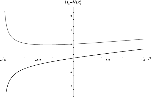 Figure 1
Peer Reviews
No public reviews on file for this paper yet. If you reviewed it on a platform where reviews are public (OpenReview, ICLR, NeurIPS, ICML), you can paste yours below so the community can read it here.
Videos
No videos yet. Explain this paper in a talk, walkthrough, or lecture? Add one.
Branched Hamiltonians for a class of
Velocity Dependent Potentials
Bijan Bagchi
Department of Physics, Shiv Nadar University, Dadri, UP 201314, India
Syed M. Kamil
Department of Physics, Shiv Nadar University, Dadri, UP 201314, India
Tarun R. Tummuru
Department of Physics, Shiv Nadar University, Dadri, UP 201314, India
Iveta Semorádová
Nuclear Physics Institute, ASCR, 250 68 e, Czech Republic
Miloslav Znojil
Nuclear Physics Institute, ASCR, 250 68 e, Czech Republic
Hamiltonians that are multivalued functions of momenta are of topical interest since they correspond to the Lagrangians containing higher-degree time derivatives. Incidentally, such classes of branched Hamiltonians lead to certain not too well understood ambiguities in the procedure of quantization. Within this framework, we pick up a model that samples the latter ambiguities and simultaneously turns out to be amenable to a transparent analytic and perturbative treatment. †† E-mails: [email protected], [email protected], [email protected],
[email protected] and [email protected]
1 Introduction
Models of classical systems with branched structures [1], in either coordinate () space or in its momentum () counterpart, have of late been a subject of active theoretical inquiry [2, 3, 4, 5, 6, 7, 9, 8]. The key idea is that classical Lagrangians possessing time derivatives in excess of quadratic powers inevitably lead to becoming a multi-valued function of velocity (), thereby yielding a multi-valued class of Hamiltonian systems.
Branched Hamiltonians in the classical context and their quantized forms have been recently discussed by Shapere and Wilczek [2]. Following it, Curtright and Zachos [3] analyzed certain representative models for a classical Lagrangian described by a pair of convex, smoothly tied functions of . Proceeding to the quantum domain shows that the double-valued Hamiltonian obtained has an inherent feature of being expressible in a supersymmetric form in the space. Subsequently, a class of nonlinear systems whose Hamiltonians exhibit branching was explored by Bagchi et al [4] who also considered the possibility of quantization for some specific cases of the underlying coupling parameter.
In this paper, we present a class of velocity-dependent Lagrangians which define a canonical momentum that yields exactly a pair of velocity variables. As a consequence, the corresponding Hamiltonians develop a branching character. An interesting aspect of our scheme is that it is well-suited for a perturbative treatment.
2 Branched Hamiltonians: A brief review
Let us briefly review the example of a branched system that was put forward in [3]. It has been noted that a typical model of branched Hamiltonians results from a non-conventional form of the Lagrangian which is given by
[TABLE]
Notice that the traditional kinetic energy term features a replacement of the quadratic form by a fractional function of velocity , while stands for a convenient local interaction potential. The fractional powers of the difference were invoked to make plausible connections to known phenomenology such as the supersymmetric pairing.
In the expression of canonical momentum derived from (1), the st root of was required to be real and positive or negative for or , respectively. The quantity , correspondingly, turns out to be a double-valued function of . Taking the Legendre transform with respect to these branches of gives rise to a pair of Hamiltonians
[TABLE]
Note that the case speaks of the canonical supersymmetric structure [10] for the difference , namely , but in the momentum space if viewed as a quantum mechanical system. The spectral and boundary condition linkages of these Hamiltonians are not difficult to set up.
3 A velocity dependent potential
Against the above background, we consider setting up of an extended Lagrangian model having a velocity dependent potential :
[TABLE]
where is defined as in Eq. (1). With and being certain functions of and respectively, we assume the potential to be given in a separable form .
Using the standard definition of the canonical momentum, we find that it is given by
[TABLE]
This relation, however, is too complicated to put down the multi-valued nature of velocity in a tractable closed form.
If we try to determine the Hamiltonian branches corresponding to this Lagrangian (3), the emerge in a mixed form involving momentum , the function and its derivative.
[TABLE]
Since the Hamiltonian has to be a function of coordinates and corresponding canonical momenta, the expression as derived above is of little use.
We note that the case is particularly interesting to understand the spectral properties of . Explicitly, the Lagrangian assumes a simple but general form
[TABLE]
A sample choice for could be
[TABLE]
with and being suitable real constants. Observe that the presence of rescales the kinetic energy coefficient which now enjoys a parametric representation.
Further, this construction of facilitates determination of the canonical momentum in a closed form, as given by
[TABLE]
where . On inversion, we find a pair of relations for the velocity that depend on :
[TABLE]
As a consequence, we run into two branches of the Hamiltonian which we write down as
[TABLE]
For the ease of notation, note that has been replaced with .
In the special case where and , we recover the Hamiltonian derived in [3]. However, the presence of the parameter in is nontrivial as our following treatment of perturbative analysis will show. In Figure 1, we have given a graphical illustration (for and ) of the behavior of the two branches of the Hamiltonian against some typical values of the momentum variable. As in the case of [3], here too, for a fixed , we encounter a cusp asymptotically with regard to .
4 Lowest excitations and the Fourier transform
After one decides to consider just small excitations of our quantum system over a local or global minimum () of a generic analytic potential , one may put the origin of the coordinate axis to this minimum, , and write down the Taylor series
[TABLE]
Recall that and the zero of the energy scale can be shifted in such a manner that . Finally, the series is truncated after the first non-trivial term yielding, in ad hoc units,
[TABLE]
After a Fourier transform to the momentum space, we get a transformed quantum form of the Hamiltonian guided by the second-order differential operator,
[TABLE]
containing a one-parametric family of pseudo-potentials
[TABLE]
Here, the original subscript ± entering Eq. (10) may be perceived as equivalent to an optional switch between positive coupling-type parameter and its negative alternative . Besides such a freedom of the sign of the dynamical characteristic, the consequent quantum-theory interpretation of the model requires also a few nontrivial mathematical addenda. The form Eq. (14) matches with Eq. (10) for which will now be our point of inquiry.
First of all, the most natural tentative candidate
[TABLE]
for the quantum Schrödinger equation living on the whole real line of momenta (i.e., with ) is characterized by the asymptotically linear decrease of the pseudo-potential (14) along the left half-line. Hence, the negative half-axis of momenta must be excluded, a priori, as unphysical. In other words, the acceptable wave functions should vanish, identically, whenever . The consistent quantization of our model must be based on the modified, half-line version of Eq. (15), viz., on Schrödinger equation
[TABLE]
such that (cf. also [2] and [3])
[TABLE]
Still, the discussion is not yet complete. Due care must be also paid to the fact that the inverse-square-root singularity of in the origin is “weak” (see, e.g., Ref. [12] for a detailed explanation of the rigorous, “extension theory” mathematical contents of this concept). In the language of physics, such a comment means that the information about possible bound states and physics represented by Eq. (16) with constraint (17) is incomplete.
In the rest of this paper (i.e., in sections 5 and 6) we shall, therefore, describe the two alternative versions of the completion of the missing, phenomenology-representing information.
5 Eligible “missing” boundary conditions at small
and
As we emphasized above, the existence of the usual discrete spectrum of bound states can only be guaranteed via an additional physical boundary condition at . Although from the point of view of pure mathematics, the choice of such a condition is flexible and more or less arbitrary, the necessary suppression of this unwanted freedom can rely upon several forms of the physics-based intuition.
Let us split the problem into two subcategories. In a simpler scenario we shall assume that the central core is repulsive and strong (i.e., that our parameter is positive and large, ). This possibility will be discussed in the next section 6. For the present, let us admit that the (real) value of is arbitrary and that the regular nature of our ordinary differential Schrödinger equation near implies that the integrability condition (17) itself still does not impose any constraint upon the energy [12]. A fully explicit and constructive demonstration of such an observation may be based on the routine reduction of (16) to its simplified, leading-order form
[TABLE]
Being valid at the very small (though still positive) values of this equation is exactly solvable in terms of Bessel functions [13]. Thus, one may choose either or .
After some algebra, we obtain the respective two-parametric families of the general solutions which depend on two parameters or and which remain energy-dependent. At small they behave, respectively, as follows,
[TABLE]
and
[TABLE]
On this purely analytic background, one of the most natural resolutions of the paradox of the ambiguity of the physical boundary conditions at may be based on the brute-force choice of the parameters or in these formulae.
Finally, let us emphasize that intuitively by far the most plausible requirement of the absence of the jump in the wave functions at , i.e., the Dirichlet boundary condition
[TABLE]
would remove the latter ambiguity of quantization in the most natural manner. The resulting pair of the requirements
[TABLE]
may be then recommended as easily derived from the well known approximate formulae for the Bessel functions near the origin [13].
6 Perturbation-theory analysis at large
In a purely formal spirit, one could complement the above recommended Dirichlet boundary condition (21) by its Neumann vanishing-derivative analogue
[TABLE]
or, more generally, by a suitable Robin boundary condition. In this context it is worth adding that with a systematic strengthening of the repulsive version of the barrier (i.e., with the growth of the positive coupling constant ) the specification of the additional boundary conditions at becomes less and less relevant because the two alternative energy levels will degenerate in the limit .
The most immediate explanation of this phenomenon may be provided by perturbation theory. In the dynamical regime, when the parameter is large, a perturbative approach seems to be particularly well suited. With , we look at the absolute minimum of the potential which occurs at , say. This value is, incidentally, unique
[TABLE]
With the construction of a Taylor series in its vicinity,
[TABLE]
we observe that the first term, which is given by
[TABLE]
in very large in this scenario. In contrast, all of the further Taylor coefficients remain very small and asymptotically negligible,
[TABLE]
Clearly then, with , can be expressed as
[TABLE]
After one re-scales the axis , Eq. (16) acquires the modified form
[TABLE]
where,
[TABLE]
One may now set
[TABLE]
yielding the very weakly perturbed harmonic-oscillator Hamiltonian
[TABLE]
In full analogy to many models with similar structure (cf., the study [11] containing further references), the exact solvability of the model in the leading-order harmonic oscillator approximation proves sufficient because in the domain of large the contribution of the anharmonic corrections becomes negligible.
7 Summary
To summarize, we looked at the particular example of a non-conventional Lagrangian with a velocity-dependent potential that leads to a double-valued structure of the associated Hamiltonian for some specific choice of the underlying coupling parameter. We showed that our scheme allows for a perturbative analysis by constructing a Taylor series near the vicinity of the absolute minimum of the potential.
8 Acknowledgments
For one of us (BB), it is a pleasure to thank Prof. Sara Cruz y Cruz and Prof. Oscar Rosas-Ortiz for warm hospitality during Quantum Fest 2016 held at UPIITA-IPN, Mexico City. MZ acknowledges the short-stay hospitality by Shiv Nadar University and the support by the GAČR Grant Nr. 16-22945S. We also all thank Prof. Bhabani Prasad Mandal for fruitful discussions.
The reference list from the paper itself. Each links out to its DOI / PubMed record.
- 1[1] M. Henneaux, C. Teitelboim and J. Zanelli Phys. Rev. A 36 (1987) 4417.
- 2[2] A. Shapere and F. Wilczek, Phys. Rev. Lett. 109 (2012) 200402, ar Xiv:1207.2677
- 3[3] T. L. Curtright and C. K. Zachos, J. Phys. A: Math. Gen. 47 (2014) 145201, ar Xiv:1311.6147
- 4[4] B. Bagchi, S. Modak, P. K. Panigrahi, F. Ruzicka and M. Znojil Mod. Phys. Lett. A 30 (2015) 1550213, ar Xiv:1505.07552
- 5[5] L. Zhao, P. Yu and W. Xu, Mod. Phys. Lett. A 28 (2013) 1350002, ar Xiv:1208.5974
- 6[6] H-H. Chi and H-J. He, Nucl. Phys. B 885 (2014) 448, ar Xiv:1310.3769
- 7[7] E. Avraham and R. Brustein, Phys. Rev. D 90 (2014) 024003, ar Xiv:1401.4921
- 8[8] H.C. Rosu, S.C. Mancas and P. Chen, Phys. Scp. 90 (2015)055208, ar Xiv:1409.5365