Structural propagation in a production network with restoring substitution elasticities
Satoshi Nakano, Kazuhiko Nishimura
TL;DR
This paper models an economy-wide production network using cascading functions and hierarchical clustering to analyze how productivity shocks propagate through the network structure.
Contribution
It introduces a novel modeling approach that captures intra-sectoral processes and restores elasticities, accurately replicating observed price and input share data over time.
Findings
The model replicates multi-sectoral price and share data accurately.
Hierarchical clustering reveals how productivity shocks propagate.
The approach links network structure to economic dynamics.
Abstract
We model an economy-wide production network by cascading binary compounding functions, based on the sequential processing nature of the production activities. As we observe a hierarchy among the intermediate processes spanning the empirical input--output transactions, we utilize a stylized sequence of processes for modeling the intra-sectoral production activities. Under the productivity growth that we measure jointly with the state-restoring elasticity parameters for each sectoral activity, the network of production completely replicates the records of multi-sectoral general equilibrium prices and shares for all factor inputs observed in two temporally distant states. Thereupon, we study propagation of a small exogenous productivity shock onto the structure of production networks by way of hierarchical clustering.
Click any figure to enlarge with its caption.
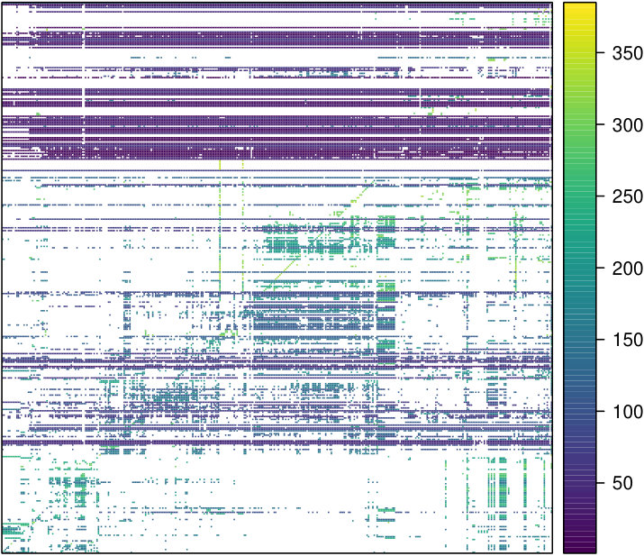 Figure 1
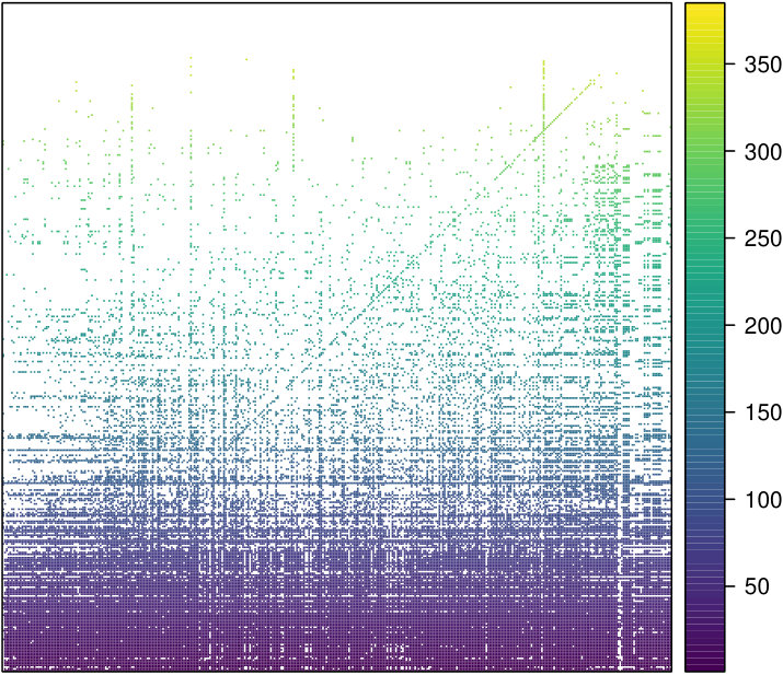 Figure 2
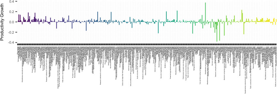 Figure 3
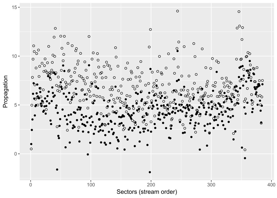 Figure 4
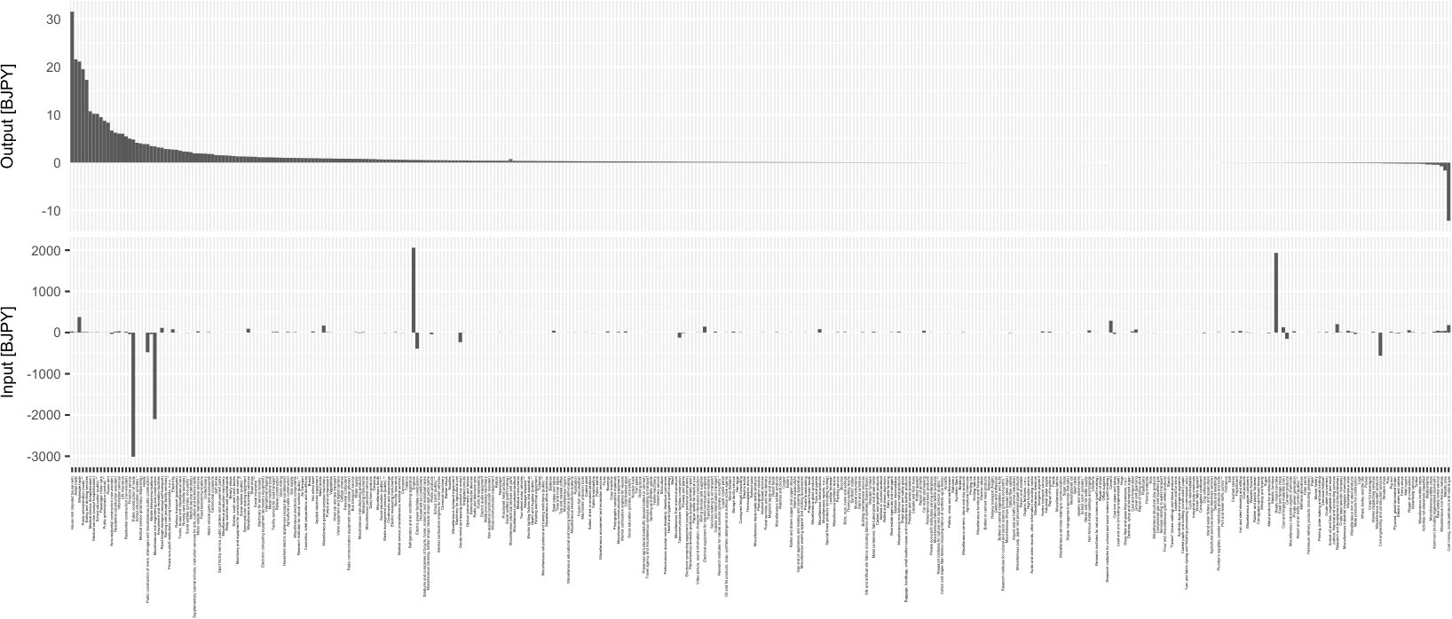 Figure 5
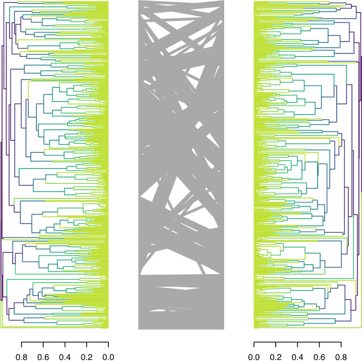 Figure 6
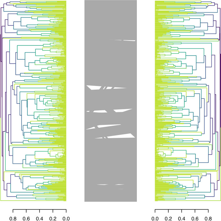 Figure 7
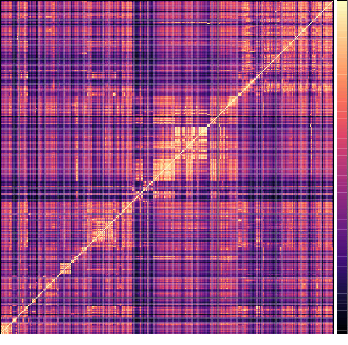 Figure 8
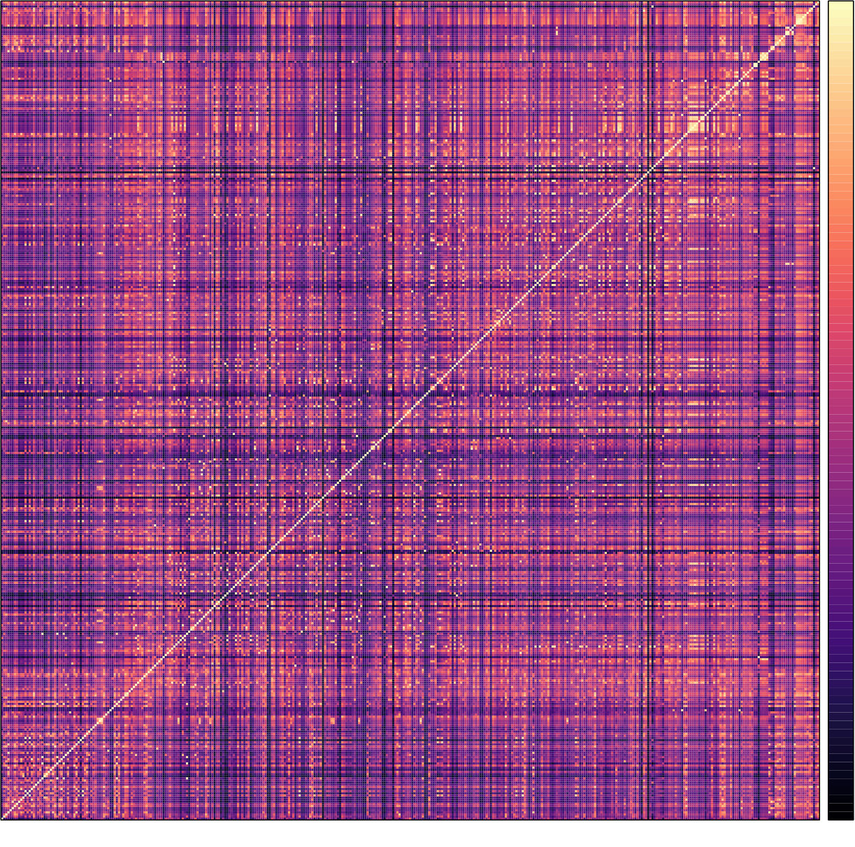 Figure 9
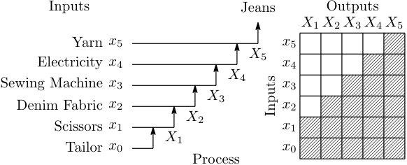 Figure 10
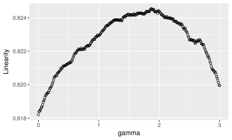 Figure 11
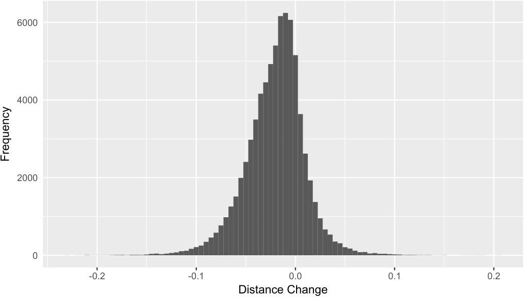 Figure 12
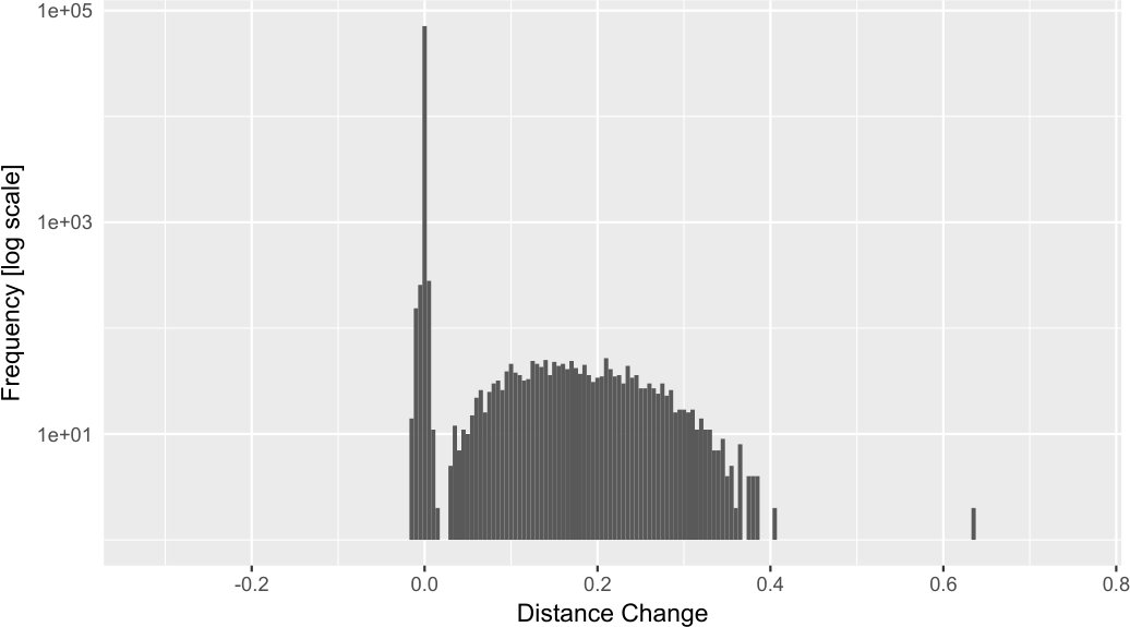 Figure 13
 Figure 14
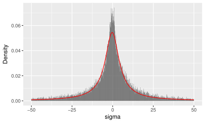 Figure 15
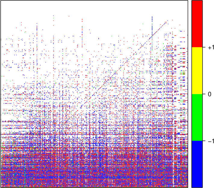 Figure 16
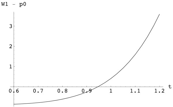 Figure 17
| Variable | Reference | Current | Projected | |
|---|---|---|---|---|
| Price | 1 | |||
| Cost share | ||||
| Productivity | 1 |
| unit: [MJPY] | Current | Projected (Leontief) | Projected (CCES) |
|---|---|---|---|
| Törnqvist | ||||||
|---|---|---|---|---|---|---|
| output | 0.8 | |||||
| input 2 | 0.3 | 0.2 | 1.2 | 1.88 | ||
| input 1 | 0.5 | 0.7 | 0.6 | 3.54 | ||
| input 0 | 0.2 | 0.1 | 0.9 |
Peer Reviews
No public reviews on file for this paper yet. If you reviewed it on a platform where reviews are public (OpenReview, ICLR, NeurIPS, ICML), you can paste yours below so the community can read it here.
Videos
No videos yet. Explain this paper in a talk, walkthrough, or lecture? Add one.
Taxonomy
TopicsComplex Systems and Time Series Analysis · Economic theories and models
Structural propagation in a production network with
restoring substitution elasticities
Satoshi Nakano
Kazuhiko Nishimura
The Japan Institute for Labour Policy and Training, Tokyo 177-0044, Japan
Faculty of Economics, Nihon Fukushi University, Aichi 477-0031, Japan
Abstract
We model an economy-wide production network by cascading binary compounding functions, based on the sequential processing nature of the production activities. As we observe a hierarchy among the intermediate processes spanning the empirical input–output transactions, we utilize a stylized sequence of processes for modeling the intra-sectoral production activities. Under the productivity growth that we measure jointly with the state-restoring elasticity parameters for each sectoral activity, the network of production completely replicates the records of multi-sectoral general equilibrium prices and shares for all factor inputs observed in two temporally distant states. Thereupon, we study propagation of a small exogenous productivity shock onto the structure of production networks by way of hierarchical clustering.
keywords:
Elasticity of Substitution , Productivity Growth , Linked Input-Output Tables , Hierarchical Clustering
††journal: International Journal of Production Economics
1 Introduction
Given the technological interdependencies among industrial activities, innovation (in terms of productivity shock) in one industry may well produce a propagative feedback effect on the performance of economy-wide production. Previous literature pertaining to the study of innovation propagation has based its theory upon the non-substitution theorem [e.g., Georgescu-Roegen, 1951] that allows one to study under a fixed technological structure while restricting the analyses to changes in the net outputs [e.g., Contreras and Fagiolo, 2014, Tsekeris, 2017]. Otherwise, Acemoglu et al. [2012] assume Cobb-Douglas production (i.e., unit substitution elasticity) with which the structural transformation is restricted to the extent that the cost-share structures are preserved. To study propagation in regard to potential technological substitutions, however, a potential range of alternative technologies must be known in advance. Nonetheless, empirical estimation of the substitution elasticities [e.g., Dixon and Jorgenson, 2013] is elusive, and to this end, the dimension of the working variables has been significantly limited.
In contrast, this study is concerned with the economy-wide propagation of innovation that involves structural transformation with regard to the potential range of technologies among input variables of large (385) dimension. In so doing we model multiple-input production activity by serially nesting (i.e., cascading) binary-input production functions of different substitution elasticities. For each industry (or sector of an economy), the elasticity parameters of the production function are measured jointly with the productivity changes so that the economy-wide production system completely replicates monetary and physical inputs in all sectors for two temporally distant equilibrium states. These elasticity parameters are hence called as restoring elasticities.
In the following, we give our rationale for modeling production by nesting binary compounding functions. Consider, say, the manufacture of a pair of jeans. For this case, one needs a sufficient amount of denim fabric, a pair of scissors, a sewing machine, a ball of yarn, some electricity, and a tailor. We know that a pair of jeans will not fall into place all at once but rather it is made in a step-by-step fashion: using a pair of scissors and a sewing machine, the fabric is first cut into pieces, then they are sewn together using the yarn with some help from electric power. Production generally involves a series of processes that combine the output of a previous process with another input of production, before handing the output over to the next process.
A production activity can be configured as a tree diagram such as the one shown in Fig. 1 (left). In this example, the production system comprises a series of six inputs , , , , , , processed in a hierarchical manner, producing five intermediate outputs, , by five processes that are nested serially. Naturally, one may be concerned that the denim fabric, for example, is produced by another (satellite) system, and therefore the extended system is inclusive of a parallel nest. Suppose, for simplicity, that denim fabric is produced by a serially nested process of two factor inputs, say, the indigo-dyed wrap and the plain weft threads, . Notice that we may always re-configure a production system into a sequence by decomposing the satellite process. In this case, denim fabric is decomposed into a sequence of two inputs (wrap and weft) and a set of cut fabric (i.e., ) is, presumably, produced by the sequence (wrap, weft, tailor, scissors), in which case, the sequence of the inputs of the extended system becomes . 111Of course, the weaving process of the threads requires a weaver. Then, the same kind of input (labor) is put into process at different stages (weaving and tailoring). By allowing indirect inputs we merge these inputs into the lower stage.
A cascaded configuration of processes can be transcribed into a triangular incidence matrix, as shown in Fig. 1. The shaded intersections represent the direct and indirect inputs and the distribution of outputs, while indirect feedbacks are ruled out for simplicity.222Indirect feedback may be, for example, the case where is fed back into . We rule this case out because there will be no way of producing the first pair of Jeans. A notable feature of this configuration is that every intermediate process constitutes a part in the overall sequence of processes. For instance, the intermediate process that produces output consists of four direct and indirect inputs, namely, , that are processed in this sequence. The overall sequence of processes is of the final output , which is , so the intermediate process obviously constitutes a part in the overall sequence. Thus, the sequence of every intermediate process is knowable by investigating the overall sequence of the triangular incidence matrix.
Our sector-level modeling of serially nested production activities requires the identification of the sequence of inputs (intra-sectoral processes) for all sectors constituting the economy, and for that matter, we utilize the economy-wide inter-sectoral transactions recorded in an input–output table. We note that, if the incidence matrix transcribed from the input–output table is completely triangular, every sector-level sequence of processes becomes known from the sequence of intermediate processes stylized in the triangulated incidence matrix. We hereafter refer to this sequence as the universal processing sequence (UPS). We will find that the input–output incidence matrix of the 2005 Japanese economy is not completely yet not too far from being triangular. From an empirical perspective, we exploit the universal sequence of processes observed through the triangulation of the input–output incidence matrix. Square matrix triangulation [e.g., Chaovalitwongse et al., 2011, Ceberio et al., 2015] refers to a generic technique for finding a simultaneous permutation of the rows and columns such that the sum of the entries above the main diagonal is maximized.
Given the hierarchical sequence of the inputs, we shall proceed to set up a production function that reflects the actual range of potential technologies. In this study, we use the constant elasticity of substitution (CES) function Arrow et al. [1961] for modeling the binary compounding process. CES has been applied exensively [e.g., Ramcharran, 2001]. Nesting CES functions creates a Cascaded CES function whose nest elasticities are the main subject of estimation. As we show later on, the restoring nest elasticities will be resolved through calibration of the sectoral productivities, in order that the two temporally distant equilibrium states, regarding prices and shares of inputs spanning all sectoral productions, are replicated. 333Previous models are calibrated at one point Rutherford [1999], while our model is subject to two-point calibration.
The calibrated multi-sectoral Cascaded CES general equilibrium model is used to simulate the production networks transformation ex post of some external productivity shock, and account for its economy-wide influences in terms of welfare measured by the gains in the final demand. Finally, we perform hierarchical cluster analysis upon the networks of production in different equilibria to study the potential structural propagation of the external productivity shock. The clustering of production networks is studied in various ways [e.g., Blöchl et al., 2011, Hu et al., 2017, Sun et al., 2018] In this study, we base our cluster evaluation on the Leontief inverse which is particular case of Katz-Bonacich centrality [Carvalho, 2014]. Upon performing hierarchical cluster analysis [e.g., Newman and Girvan, 2004, McNerney et al., 2013] we measure sectoral distances based on Pearson’s correlation between sectoral multipliers of the changing production networks.
In section 2, we explain how the elasticity parameters and the productivity change of a Cascaded CES function are calibrated, given the universal processing sequence. In section 3, we demonstrate that the equilibrium structures for both reference and current states are replicated, and how the production network is transformed by an exogenous productivity stimulus. Section 4 provides concluding remarks. Note that superscripts are hereafter reserved for exponents, while subscripts are for indicating variety of inputs, nests, and industries, but not for partial derivatives. The notation for key variables in different states is summarized in Table 1.
2 Model
2.1 Cascaded CES Function
Suppose that UPS of inputs is known. Then, a cascaded (i.e., serially nested) production function of inputs for an industry (whose index is omitted) can be described as follows:
[TABLE]
Here, is the output, is the th input, and is the productivity level. There are nests, each consisting of one factor input and a compound from the lower level nest, except for the primary nest, which includes two non-compound inputs. Note that we allow to decrease (i.e., production activity may lose output performance instead of gaining), as may be observed in reality. We define , for convenience.
The CES production function for the th compound output processed at the th nest is of the following form:
[TABLE]
The nest production function (1) holds for , since there are nests in a production activity. Here, is the share parameter of the th nest, is the compound output from the th nest, and is the elasticity of substitution between th input and the compound input from the lower level nest . We assume that (1) is homogeneous of degree one.
The following is the dual (or unit cost) function of the th compound output given in (1):
[TABLE]
Here, is the price of the th input, and is the price of the compound input from the lower level nest. We may verify that (2) is a dual function of (1) by the following exposition. First, as we presume zero profit in the nest process, the following identity must hold:
[TABLE]
Then, by virtue of (1) and (3), we have
[TABLE]
Alternatively, by virtue of (2) and (3), we have
[TABLE]
Hence, it is safe to say that (2) is the unit cost function of (1), since (4) and (5) are equivalent. A Cascaded CES unit cost function can then be created by nesting (2) serially as follows:
[TABLE]
where indicates the unit cost of the sector concerned. For convenience, we may define that .
2.2 Restoring Elasticities
A worked example of the calibration procedure that we present in this section for a two-stage Cascaded CES function is given in A. To begin with, let us apply Euler’s homogeneous function theorem and the no-arbitrage (i.e., zero profit) condition to the unit cost function:
[TABLE]
By recursively taking the derivatives for (2), we arrive at the following identities for :
[TABLE]
Then, the cost share of the input of the th nest, counting from the outermost of the nests, which we denote by , can be derived as a function of the prices of the compound inputs, as follows:
[TABLE]
Our task here is to solve for for all and the change in , using the shares and prices observed in two different states, namely, the current and the reference. First, we standardize all prices by those of the inputs (and outputs) of the reference state and set them at unity, i.e., , while denoting the reference-standardized prices of the current state by . The productivity level for the reference state must also be standardized and set to unity, i.e., , since we know from (2) that for all . We also let be given outside of the system, because the primary input (i.e., numéraire good or labor) is not produced industrially.
We denote the observed cost share of the th input of the reference state by and that of the current state by . For later convenience, we introduce , a set of observables in the two states for the th input. Further, we note that and for convenience. Applying reference state values into (7) yields the following:
[TABLE]
The following modification may not be so obvious; nonetheless, we may see the equivalence by applying all possible recursively into (8). By taking into account, Further (8) can be modified to calibrate the share parameters:
[TABLE]
Applying current state values to (7) we have:
[TABLE]
By rearranging terms, we obtain the following:
[TABLE]
We write the above in terms of its entries (unknowns and knowns separated by a semi-colon) for convenience:
[TABLE]
Also, (2) is evaluated at the current state:
[TABLE]
Again, we write the above in terms of its entries:
[TABLE]
Now, let us work on (10) and (11) step by step from the outer layer of the nests, i.e., . For this particular layer, we may resolve the unknowns, given , viz.,
[TABLE]
Note that the second equation is restating (6) at the current state . Using the above terms the compound price is evaluated as follows:
[TABLE]
We may work on a few layers below:
[TABLE]
We repeat this procedure and obtain the following series:
[TABLE]
Thus, can be calibrated by way of the condition of the final stage at the current state, i.e.,
[TABLE]
and the restoring elasticity parameters can all be resolved for , using the solution of (12), which we hereafter denote by .
3 Empirical Analysis
3.1 Universal Processing Sequence
The degree to which a macroscopic production structure agrees with the hierarchical order of processing sequences is the linearity. In a perfectly linear structure, the processing sequences will only cascade from upstream to downstream; if this is the case, then we may arrange the rows and columns of the input–output matrix according to the hierarchical order to obtain a triangular matrix, and hence, the universal processing sequence.
More specifically, for an sector output system with intermediate inputs (excluding self-input), the furthest upstream (headwaters) sector has no intermediate input and output destinations (i.e., zero column and row entries) whereas the furthest downstream sector has inputs with no intermediate output destination (i.e., column and zero row entries). Let us denote a reordering of sectors whose initial order is by a permutation mapping . Further, let designate the inverse, so that a -permuted version of a matrix can be specified as follows:
[TABLE]
For later discussion, let us work on a discretized square input–output matrix (i.e., input–output incidence matrix) whose elements are binary, specifically, if transaction , and if . The linearity of a matrix with permutation is defined as follows:
[TABLE]
Note that the denominator is the sum of the off-diagonal entries of the matrix, which is constant. The numerator , on the other hand, depends on the permutation.
The triangulation problem of matrix is to find a permutation mapping that maximizes the linearity, i.e.,
[TABLE]
where is the set of all possible permutations. This problem is known as the linear ordering problem. The number of all possible permutations is as large as for an matrix, and the problem is known to be NP-hard. Thus, none of the exact methods (typically via discrete optimization) will work when one attempts to handle a matrix of 385 sectors. Hence we take a heuristic approach.
One possible approach would be to use the ratio of the input incidents total (column sum of ) to the output incidents total (row sum of ), which we denote by and define below, and to arrange the permutation in the ascending order of this ratio.
[TABLE]
This heuristic is a simple emulation of the method proposed by Chenery and Watanabe [1958], except that the original study uses the input–output coefficient matrix instead of an incidence matrix. Note that in this case the set of possible permutations contains only one element, which we denote by ; that is, . In other words, permutation is the ascending order of the above-mentioned ratios , or .
In this study, we slightly further generalize this CW heuristic. In particular, we take the weighted ratio of the input incidents total to the output incidents total, as described below, in order to expand the number of possible permutations .
[TABLE]
This ratio is inclusive of CW heuristic at . We thus evaluate the linearity of with permutation with respect to the ascending order of the ratios , such that for all .
Note that must be nonnegative, according to the purpose of triangulating matrix . Obviously, if we are to put more weight on the outputs, and if we are to put more on the inputs. Our objective is hence to search for the that maximizes the linearity, that is, to find a such that
[TABLE]
We shall hereinafter refer to the order of sectors given by as the stream order.
3.2 Data and Measurement
We base our empirical study upon Japan’s 2000–2005–2011 linked input–output tables MIAC [2016]. This set of tables includes the yearly commodity transactions of 385 factors (inputs) among the 385 industrial sectors (outputs) in Japan for three different periods. The transactions are recorded in nominal monetary values; thus, in order to enable comparison in real (or physical) quantities between different periods, nominal values are converted into real values by a set of price indexes called deflators, which are also included in a set of linked input–output tables. We thus have three input–output transaction matrices which can be converted into a series of input shares and prices spanning the three periods of observation.
When we began to study this data set, we found a considerable number of inconsistent transactions. Namely, 0.15% of the incidents that existed in 2000 had disappeared by 2005, and 0.46% of the incidents that existed in 2005 had disappeared by 2011. Likewise, 0.54% of the incidents that existed in 2005 did not exist in 2000, and 0.21% of the incidents that existed in 2011 did not exist in 2005. Such inconsistencies in transactions interfere with our calibration of the parameters; thus, we decided to use the two intermediate values of the three observations. In other words, we merged two temporally neighboring transactions and created 2000–2005 and 2005–2011 average transaction tables. We still, however, observed inconsistencies between the two incidents for, for example, the case where ; merging the neighboring transactions, i.e., , cannot circumvent this inconsistency. In such cases, to avoid inconsistencies we modified the transactions such that . Such modification was needed for 0.2% of the 2005–2011 non-zero transactions. As for prices, we used the mean values of the two temporally neighboring deflators for each commodity.
Figure 3 shows the result of performing the search for in using the incidence matrix based on 2005–2011 average input-output transactions. The solution of (13) is at . Note that for the CW heuristic, which occurs at . Figure 2 shows how the input–output incidence matrix is actually triangulated with our heuristic under . We find that sectors such as Office supplies, Water supply, Gas supply, Electricity, Construction services, and Information services, are among the upstream (at the top of the stream order), whereas Medical service, School education, Public baths, Barber shops, and Movie theaters, are among the downstream (at the bottom of the stream order).
Hereafter, we shall use the 2000–2005 average transactions as the reference and the 2005–2011 average transactions as the current. Figure 6 shows the results of a productivity calibration by solving (12) for all industries, using the reference and current input shares and deflators obtainable from the 2000–2005 average and 2005–2011 average transactions. The solution of (12), i.e., , is converted into a growth term with respect to the reference state, which we call the productivity growth . Notice that these productivity growths were almost identical to the following widely used productivity measure (i.e., total factor productivity growth, TFPg) based on Törnqvist index.
[TABLE]
Diewert [1976] showed that (14) can exactly capture the productivity growth of the underlying translog function. In Fig. 4, we show the elasticity parameters for individual nests, resolved by way of (10), (11), and (12). The elasticity parameters are represented by colors: yellow is used for , red for , blue for , and green for , as indicated in the right bar. The distribution of the elasticity parameters is shown in Fig. 5. Note that the histogram is fitted by the q-Gaussian distribution Tsallis [2009]. The main parameter was estimated to be with standard error using the method established by de Santa Helena et al. [2015], while other parameters were fitted at -mean and -variance by minimizing the residual sum of squares.
3.3 Multisectoral General Equilibrium
Let us now verify that the productivity growths we measured correctly replicate the two states, reference and current, in the light of multisectoral general equilibrium. We begin by writing (6) in vector form:
[TABLE]
where denotes a row vector of Cascaded CES unit cost functions and angle brackets indicate a diagonalized vector. The gradient of is
[TABLE]
where is a row vector, and is an matrix.
According to Shephard’s lemma, current state input shares can be described in terms of the current state (i.e., , , ) by the gradient of the unit cost function, as follows:
[TABLE]
Likewise, for the reference state (i.e., , , ), the following must hold for the reference input shares :
[TABLE]
Note that all the parameters of , i.e., , have been resolved previously, to satisfy the above four equations for the two states, through the calibration of . Thus, we verify that and can actually replicate the two equilibrium prices and , with given.
Because is homogeneous of order one in , Euler’s homogeneous function theorem is applicable for (15). At the reference state, the theorem implies that
[TABLE]
Note that the last part of the equality is due to the nature of shares: . Likewise, similar result is obtainable for the current state, as follows:
[TABLE]
We hereafter recognize as the production networks comprising the entire potential alternative technologies, or the meta structure, while representing the equilibrium production network in terms of shares of the inputs for all sectors (i.e., input–output coefficient matrix).
3.3.1 Networking Clusters in Equilibrium
In order to describe the production network in different equilibrium states, as well as to make comparisons between them, we perform cluster analysis. Technological similarity of sectors in a production network has been studied by various methods pertaining to the measurement of distances between a pair of sectors McNerney et al. [2013], Blöchl et al. [2011], Newman and Girvan [2004]. In the present study, we measure cluster distance based on the correlation between the net multipliers of two sectors. The net multiplier of sector measures the indirect requirements from all sectors needed to deliver a unit output to final demand from sector . Specifically, is an -column vector of the following identity:
[TABLE]
where represents the input–output coefficient matrix of a certain state. In other words, portrays sector ’s characteristic pattern of unit output propagation.
In Fig. 7, we display the heatmap of the correlations between all possible pairs of the net multipliers for the current state. Note that we convert Pearson correlations into the following scaled Euclidean distance:
[TABLE]
Thus, a perfect correlation has zero distance, whereas a zero correlation has a distance of and a perfect negative correlation has a distance of . The greatest distance shown in Fig. 7 is indicated by the darkest color. Notice that clustering is observable in the original order of the sector classification. This is supposedly because the sectoral classification of an input–output table is based fundamentally on Colin Clark’s three-sector theory, and the sectors are disaggregated while placed in the neighborhood. On the other hand, the clusters are homogenized more or less in the case of stream order as far as Fig. 7 is concerned.
3.3.2 Networking Clusters Transformation
We further examine the changes in the networking clusters in different states. However, we found that the changes in the multiplier correlations between different equilibrium states were visually undetectable by way of a heatmap. Hence, we examine the transformation of the networking clusters by way of the changes in the correlation distances between all possible pairs of the multipliers. In Fig. 8, we show the results of hierarchical clustering using dendrograms for the reference and current distance metrics of the correlations between the net multipliers. In Fig. 9, we display a histogram of the differences of distance between the two states. Overall, the distances have contracted in the current state relative to the reference state.
Given the meta structure , we may project the equilibrium state, given an exogenous productivity shock . The projected equilibrium price is the solution to the following system of equations:
[TABLE]
The solution can be obtained by iteration, if the given productivity shock is enhancing, i.e., for all , since the domain will be contracting during this iteration process. The iteration begins with the current equilibrium price; thus, the initial guess of the equilibrium price is . The recurrence formula for can be described as follows:
[TABLE]
Specifically, the domain will be contracted
[TABLE]
Hence, (16) is a contraction mapping that converges monotonically to the equilibrium such that . Note that we only used the monotonicity of to show the convergence of the process (16) for the enhancing case (i.e., ). For a non-enhancing case, we need a guarantee that an equilibrium exists, which is provided if is a concave mapping Krasnosel’skiĭ [1964]; we may then take any initial guess to arrive at the equilibrium via (16).
The social benefit of innovation (in terms of enhanced productivity ) relative to the current state must be the reduced projected price of commodities . In this study, we evaluate such social benefit by the increase in earnable final demand for the same total amount of the primary input. In other words, we evaluate innovation in terms of how much more net output can be provided from the same total amount of primary input. For later convenience, we introduce the projected input–output coefficients ex post of over current state as follows:
[TABLE]
Then, our innovation assessment problem can be specified as the following:
[TABLE]
where is the current-state net output (or final demand) observed in the form of a column vector, while is the scalar to be maximized. Note that the right-hand side of the constraint is the total of primary inputs of the current state, and the objective term is the total earnable final demand at the projected state whose commodity-wise proportion is fixed at the current state. The solution of the problem can be obtained by the following calculation:
[TABLE]
Further, we may examine the distribution of the primary inputs in the current and projected states, as follows:
[TABLE]
Here, denotes the redistribution of the primary inputs, whose entries will sum to zero. Moreover, we may calculate the economic welfare gain provided by , as the gain in the final demand, as follows:
[TABLE]
Note that is the aggregated demand, which equals the GDP of the current state economy.
3.3.3 Structural Propagation of RMC110
Here, we examine the structural propagation effect of an RMC110 innovation (where “RMC” refers to the “Ready mixed concrete” sector and “110” indicates a 10% productivity increase) injected into the current state economy. RMC110 is specifically the following vector:
[TABLE]
Note that RMC appears 145th in the original order and 244th in the (upstream-first) stream order. The empirically observed Törnqvist index value is approximately for the interval between the reference and current states. By recursive means, is obtained via (16) under (17), and accordingly, the ex post equilibrium structure () is obtained as well. We calculate the scaled Euclidean distances between the net multipliers of and compare them with those of in Fig. 11. Since RMC110 is a very small injected productivity shock 444Japan’s GDP of the current state was BJPY, while the output of the RMC sector was BJPY. Thus, 10% of the current RMC output amounts to 0.0243% of the current GDP. , the scaled Euclidean distances of the output multipliers have changed just slightly towards sparsity. In Fig. 10, we show the tanglegram comprising the results of hierarchical clustering for the current and projected distance metrics of the correlations between the multipliers. Note that the right-hand tree of Fig. 8 is identical to the left-hand tree of Fig. 10. The clusters have transformed to a certain extent between the reference and current states, as well as slightly between the current state and the projected state given by RMC110.
Figure 12 displays the log-absolute difference between current and projected primary inputs in stream order, under Cascaded CES (open dots) and Leontief (filled dots) networks. Note that Leontief network eliminates any sort of technology substitution (i.e., assuming for all and ). Structural propagation under Cascaded CES network clearly outperforms non-structural propagation under Leontief meta structure.
Table 2 summarizes the welfare calculation with regard to structural propagation of RMC110 applied to the current state. Here, and indicate gross output and value added, respectively, of the RMC sector. The breakdown of indicates that primary inputs are to be redistributed to sectors such as Engine, Ready mixed concrete, and Wholesale trade, from sectors such as Public construction of roads, Miscellaneous civil engineering, and Civil engineering and construction services, in order to gain an economic welfare equivalent to MJPY, given by RMC110. Further, note that a crude evaluation of RMC110 is to note first that 10% of the current state output of RMC amounts to MJPY. This is the amount that the RMC sector is able to gain initially from RMC110. In contrast, the propagation effect that pertains to the total amount of welfare gain, even without technological substitution (Leontief), can be almost two-fold larger (), and would be three-fold larger () if we were to consider the full propagation effect, inclusive of the potential structural change.
4 Concluding Remarks
Unlike utility, production is a step-by-step practice. Accordingly, we took into account the configuration of the processes that underlie a production activity. We broke down the configuration of production into activities that comprised binary and nested processes. For empirical purposes, we applied a CES function for each nest process, resulting in a Cascaded CES function for modeling industrial production. Moreover, we used the sequence of inputs obtained by the triangulated input–output incidence matrix for modeling the intra-sectoral sequence of processes, as we observed a stylized hierarchy among the intermediate processes spanning the empirical input–output transactions.
By using linked input–output tables as the two-point data source, the elasticity parameters of Cascaded CES functions were resolved synchronously though the calibration of productivity. At the same time, substantial negative nest elasticity parameters and productivity growths were observed. These amounts being negative may be attributed to bias in price measurement in the presence of qualitative changes. Still, these parameters caused no problems, as far as the general equilibrium analysis was concerned. The credibility of the calibrated system is validated by the complete replication of the two observed states portrayed in the linked input–output tables. Naturally, the analysis becomes more decisive when we advance the study to work more on capital and growth, quality considerations, and international trade, all of which remain for further investigation.
Appendix A Two-stage Cascaded CES calibration
We start with a following two-stage Cascaded CES function, where .
[TABLE]
This is the two-stage () version of the function defined in (2) and (6). As regards (9), the share parameters are equalt to the cost shares at the reference state:
[TABLE]
The following exposition shows the procedure for parameter calibration via backward induction:
[TABLE]
Hence, we can calibrate for the final condition, which is the two-stage version of (12):
[TABLE]
For demonstration purposes, we calibrate on the data given in Table 3. We use the data, i.e., and for calibrating . Note that and are not used in the calculation, because the shares are degenerate, i.e., . Figure 13 illustrates how (18) is solved for ; the solution is listed in Table 3. We also include TFPg calculable from the same data, using (14). The elasticity parameters and are resolved at the calibrated productivity .
References
- Acemoglu et al. [2012]
Acemoglu, D., Carvalho, V.M., Ozdaglar, A., Tahbaz-Salehi, A., 2012.
The network origins of aggregate fluctuations.
Econometrica 80, 1977 – 2016.
doi:10.3982/ECTA9623.
- Arrow et al. [1961]
Arrow, K.J., Chenery, H.B., Minhas, B.S., Solow, R.M., 1961.
Capital-labor substitution and economic efficiencys.
Review of Economics and Statistics 43, 225–250.
- Blöchl et al. [2011]
Blöchl, F., Theis, F.J., Vega-Redondo, F., Fisher, E.O., 2011.
Vertex centralities in input-output networks reveal the structure of modern economies.
Physical Review E 83, 046127.
- Carvalho [2014]
Carvalho, V.M., 2014.
From micro to macro via production networks.
Journal of Economic Perspectives 28, 23–48.
doi:10.1257/jep.28.4.23.
- Ceberio et al. [2015]
Ceberio, J., Mendiburu, A., Lozano, J.A., 2015.
The linear ordering problem revisited.
European Journal of Operational Research 241, 686 – 696.
doi:10.1016/j.ejor.2014.09.041.
- Chaovalitwongse et al. [2011]
Chaovalitwongse, W.A., Oliveira, C.A.S., Chiarini, B., Pardalos, P.M., Resende, M.G.C., 2011.
Revised grasp with path-relinking for the linear ordering problem.
Journal of Combinatorial Optimization 22, 572–593.
doi:10.1007/s10878-010-9306-x.
- Chenery and Watanabe [1958]
Chenery, H.B., Watanabe, T., 1958.
International comparisons of the structure of production.
Econometrica 26, 487–521.
- Contreras and Fagiolo [2014]
Contreras, M.G.A., Fagiolo, G., 2014.
Propagation of economic shocks in input–output networks: A cross-country analysis.
Physical Review E 90, 062812.
- Diewert [1976]
Diewert, W.E., 1976.
Exact and superlative index numbers.
Journal of Econometrics 4, 115–145.
- Dixon and Jorgenson [2013]
Dixon, P.B., Jorgenson, D.W. (Eds.), 2013.
Handbook of Computable General Equilibrium Modeling. volume 1A of Handbooks in Economics.
Elsevier, North Holland.
- Georgescu-Roegen [1951]
Georgescu-Roegen, N., 1951.
in: Koopmans, T. (Ed.), Activity Analysis of Production and Allocation. John Wiley and Sons, Inc.. chapter Some Properties of a Generalized Leontief Model, pp. 165–173.
- Hu et al. [2017]
Hu, F., Zhao, S., Bing, T., Chang, Y., 2017.
Hierarchy in industrial structure: The cases of china and the usa.
Physica A 469, 871 – 882.
doi:10.1016/j.physa.2016.11.083.
- Krasnosel’skiĭ [1964]
Krasnosel’skiĭ, M.A., 1964.
Positive Solutions of Operator Equations.
Groningen, P. Noordhoff.
- McNerney et al. [2013]
McNerney, J., Fath, B.D., Silverberg, G., 2013.
Network structure of inter-industry flows.
Physica A 392, 6427 – 6441.
doi:10.1016/j.physa.2013.07.063.
- MIAC [2016]
MIAC, 2016.
Ministry of Internal Affairs and Communications 2000–2005–2011 Linked Input-Output Tables [in Japanese].
URL: http://www.soumu.go.jp.
- Newman and Girvan [2004]
Newman, M.E.J., Girvan, M., 2004.
Finding and evaluating community structure in networks.
Physical Review E 69, 026113.
- Ramcharran [2001]
Ramcharran, H., 2001.
Productivity, returns to scale and the elasticity of factor substitution in the usa apparel industry.
International Journal of Production Economics 73, 285 – 291.
doi:10.1016/S0925-5273(01)00100-1.
- Rutherford [1999]
Rutherford, T.F., 1999.
Applied general equilibrium modeling with mpsge as a gams subsystem: An overview of the modeling framework and syntax.
Computational Economics 14, 1–46.
- de Santa Helena et al. [2015]
de Santa Helena, E., Nascimento, C., Gerhardt, G., 2015.
Alternative way to characterize a q-gaussian distribution by a robust heavy tail measurement.
Physica A 435, 44 – 50.
doi:10.1016/j.physa.2015.04.032.
- Sun et al. [2018]
Sun, X., An, H., Liu, X., 2018.
Network analysis of chinese provincial economies.
Physica A 492, 1168 – 1180.
doi:10.1016/j.physa.2017.11.045.
- Tsallis [2009]
Tsallis, C., 2009.
Introduction to Nonextensive Statistical Mechanics: Approaching a Complex World /.
Springer New York,, New York, NY :.
- Tsekeris [2017]
Tsekeris, T., 2017.
Global value chains: Building blocks and network dynamics.
Physica A 488, 187 – 204.
The reference list from the paper itself. Each links out to its DOI / PubMed record.
- 1Acemoglu et al. [2012] Acemoglu, D., Carvalho, V.M., Ozdaglar, A., Tahbaz-Salehi, A., 2012. The network origins of aggregate fluctuations. Econometrica 80, 1977 – 2016. doi: 10.3982/ECTA 9623 . · doi ↗
- 2Arrow et al. [1961] Arrow, K.J., Chenery, H.B., Minhas, B.S., Solow, R.M., 1961. Capital-labor substitution and economic efficiencys. Review of Economics and Statistics 43, 225–250.
- 3Blöchl et al. [2011] Blöchl, F., Theis, F.J., Vega-Redondo, F., Fisher, E.O., 2011. Vertex centralities in input-output networks reveal the structure of modern economies. Physical Review E 83, 046127.
- 4Carvalho [2014] Carvalho, V.M., 2014. From micro to macro via production networks. Journal of Economic Perspectives 28, 23–48. doi: 10.1257/jep.28.4.23 . · doi ↗
- 5Ceberio et al. [2015] Ceberio, J., Mendiburu, A., Lozano, J.A., 2015. The linear ordering problem revisited. European Journal of Operational Research 241, 686 – 696. doi: 10.1016/j.ejor.2014.09.041 . · doi ↗
- 6Chaovalitwongse et al. [2011] Chaovalitwongse, W.A., Oliveira, C.A.S., Chiarini, B., Pardalos, P.M., Resende, M.G.C., 2011. Revised grasp with path-relinking for the linear ordering problem. Journal of Combinatorial Optimization 22, 572–593. doi: 10.1007/s 10878-010-9306-x . · doi ↗
- 7Chenery and Watanabe [1958] Chenery, H.B., Watanabe, T., 1958. International comparisons of the structure of production. Econometrica 26, 487–521.
- 8Contreras and Fagiolo [2014] Contreras, M.G.A., Fagiolo, G., 2014. Propagation of economic shocks in input–output networks: A cross-country analysis. Physical Review E 90, 062812.