Star formation driven galactic winds in UGC 10043
C. L\'opez-Cob\'a, S. F. S\'anchez, A. V. Moiseev, D. V. Oparin, T., Bitsakis, I. Cruz-Gonz\'alez, C. Morisset, L. Galbany, J. Bland-Hawthorn, M., M. Roth, R.-J. Dettmar, D. J. Bomans, R. M. Gonz\'alez Delgado, M., Cano-D\'iaz, R. A. Marino, C. Kehrig, A. Monreal Ibero

TL;DR
This study investigates the ionized gas outflows in galaxy UGC 10043, revealing shock-ionized winds reaching up to 4 kpc, with detailed analysis of their physical properties using multiple observational techniques.
Contribution
It combines integral field spectroscopy, Fabry-Perot interferometry, and photometry with shock models to characterize galactic winds in UGC 10043, providing new insights into outflow properties.
Findings
Ionized gas detected up to 4 kpc above the disk.
Gas velocities increase up to 400 km/s along the outflow.
Discrepancy between SFR estimates from Ha and CIGALE.
Abstract
We study the galactic wind in the edge-on spiral galaxy UGC 10043 with the combination of the CALIFA integral field spectroscopy data, scanning Fabry-Perot interferometry (FPI), and multiband photometry. We detect ionized gas in the extraplanar regions reaching a relatively high distance, up to ~ 4 kpc above the galactic disk. The ionized gas line ratios ([N ii]/Ha, [S ii]/Ha and [O i]/Ha) present an enhancement along the semi minor axis, in contrast with the values found at the disk, where they are compatible with ionization due to H ii-regions. These differences, together with the biconic symmetry of the extra-planar ionized structure, makes UGC 10043 a clear candidate for a galaxy with gas outflows ionizated by shocks. From the comparison of shock models with the observed line ratios, and the kinematics observed from the FPI data, we constrain the physical properties of the observed…
Click any figure to enlarge with its caption.
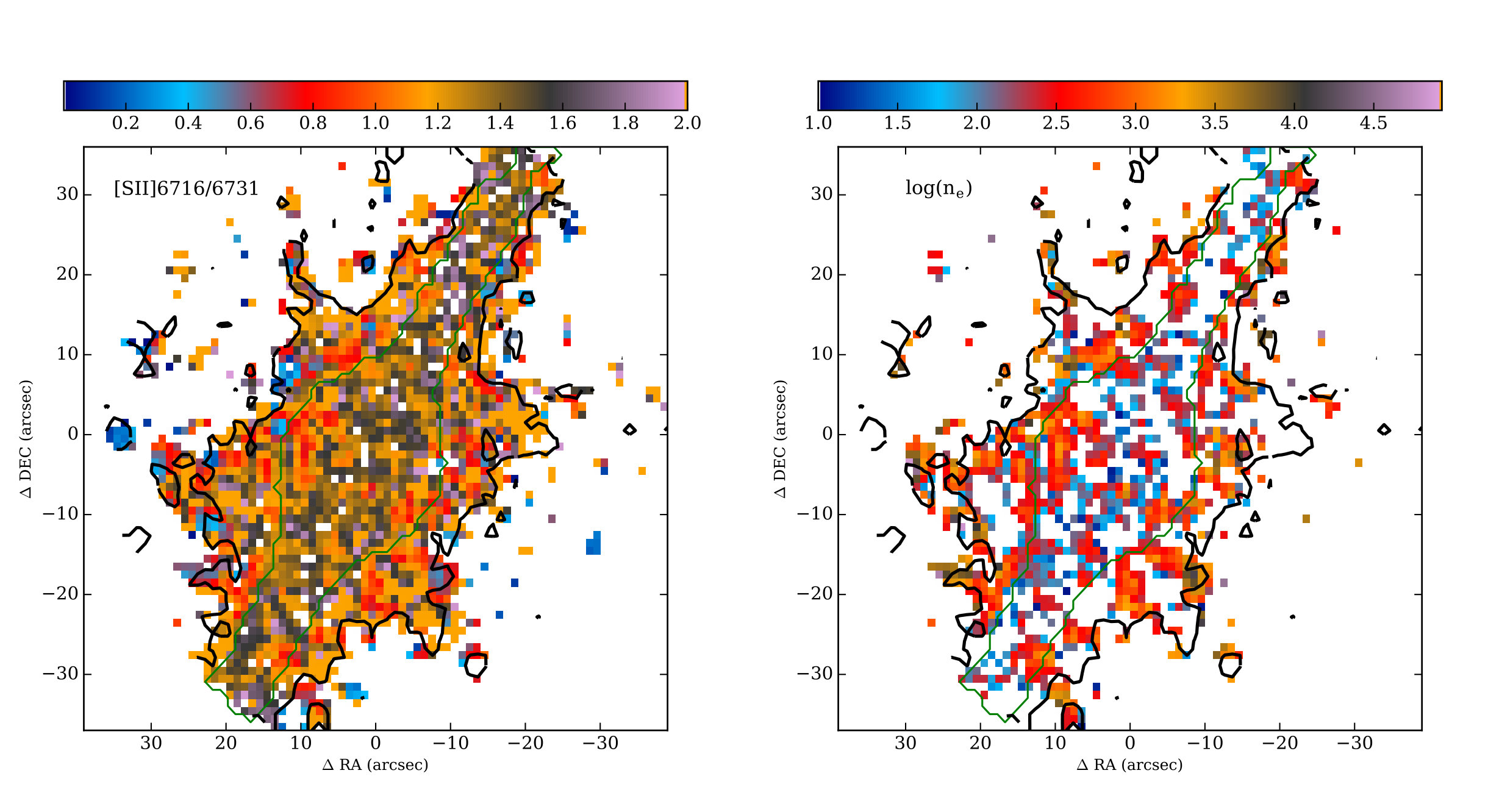 Figure 1
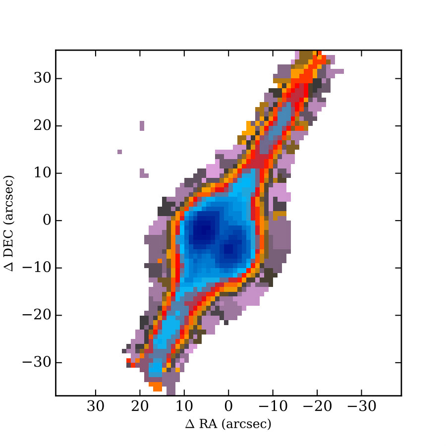 Figure 2
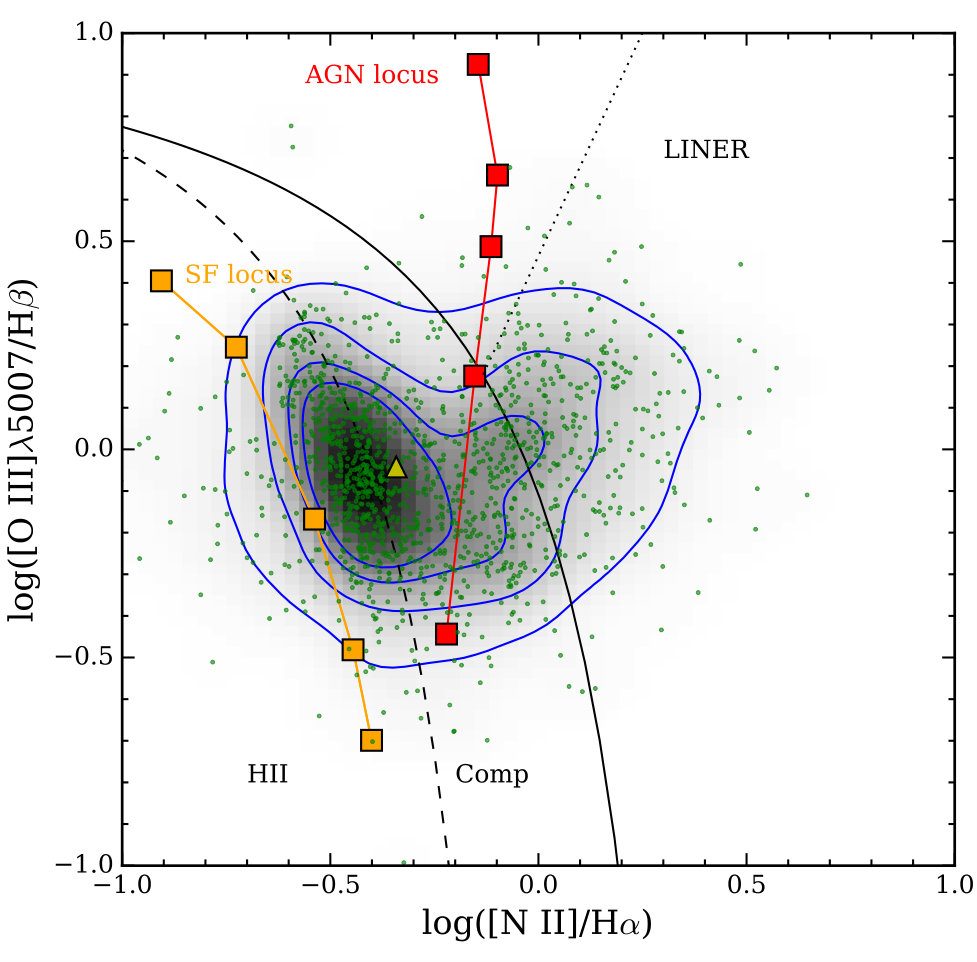 Figure 3
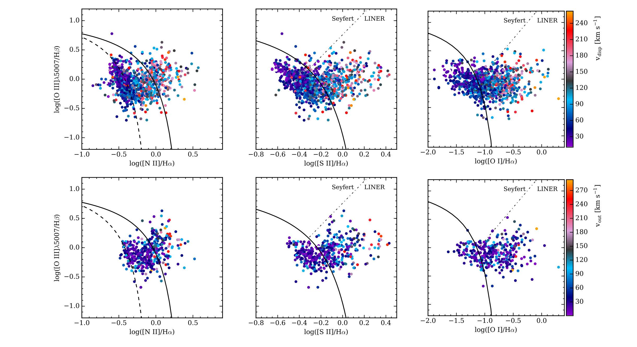 Figure 1
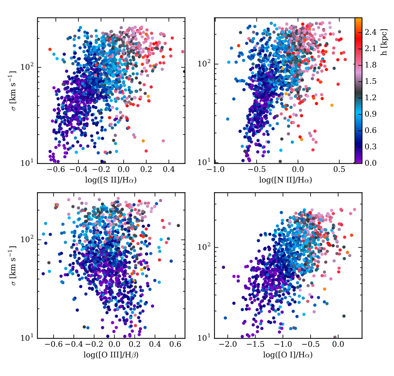 Figure 1
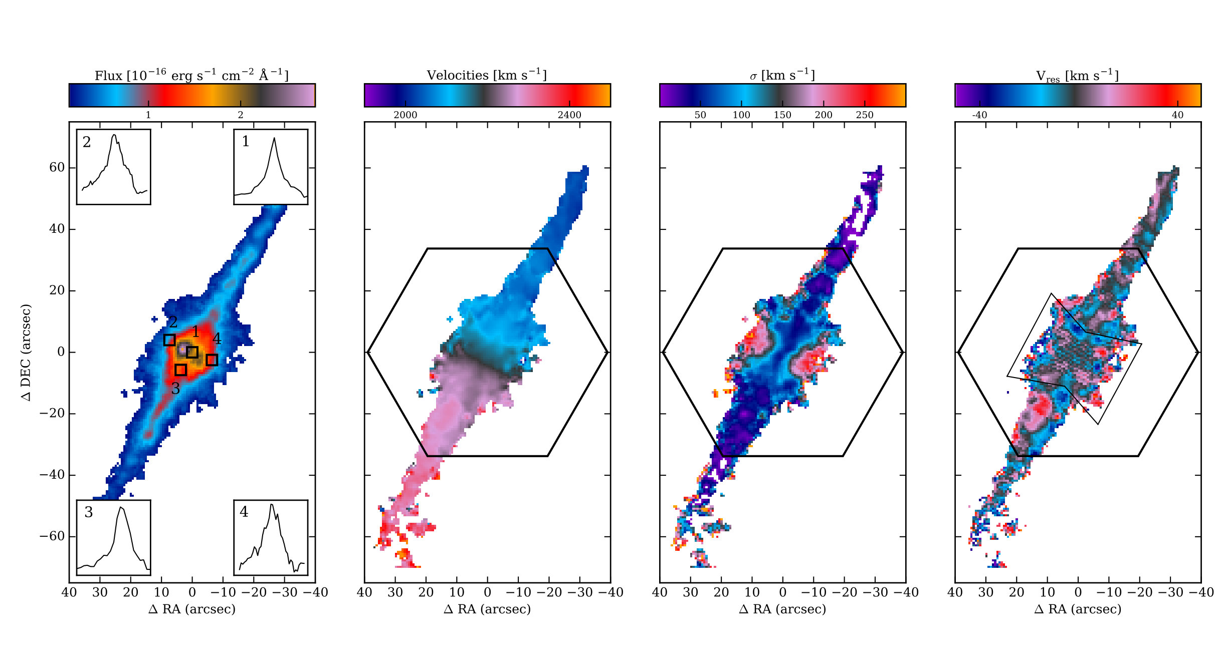 Figure 6
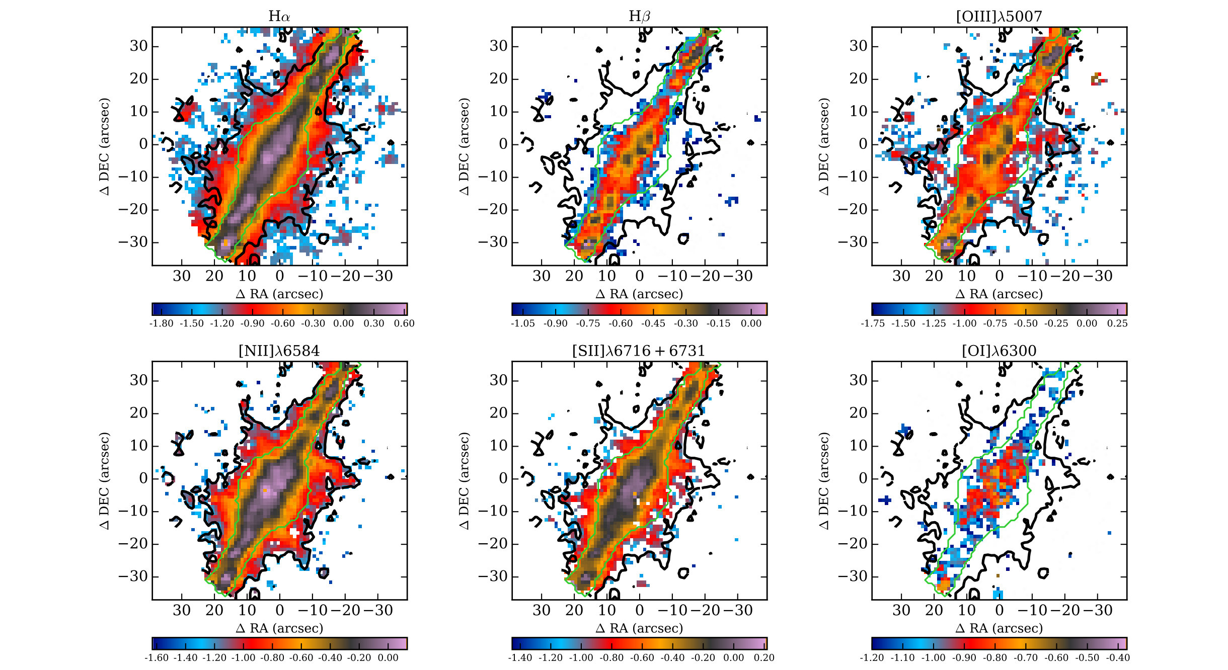 Figure 7
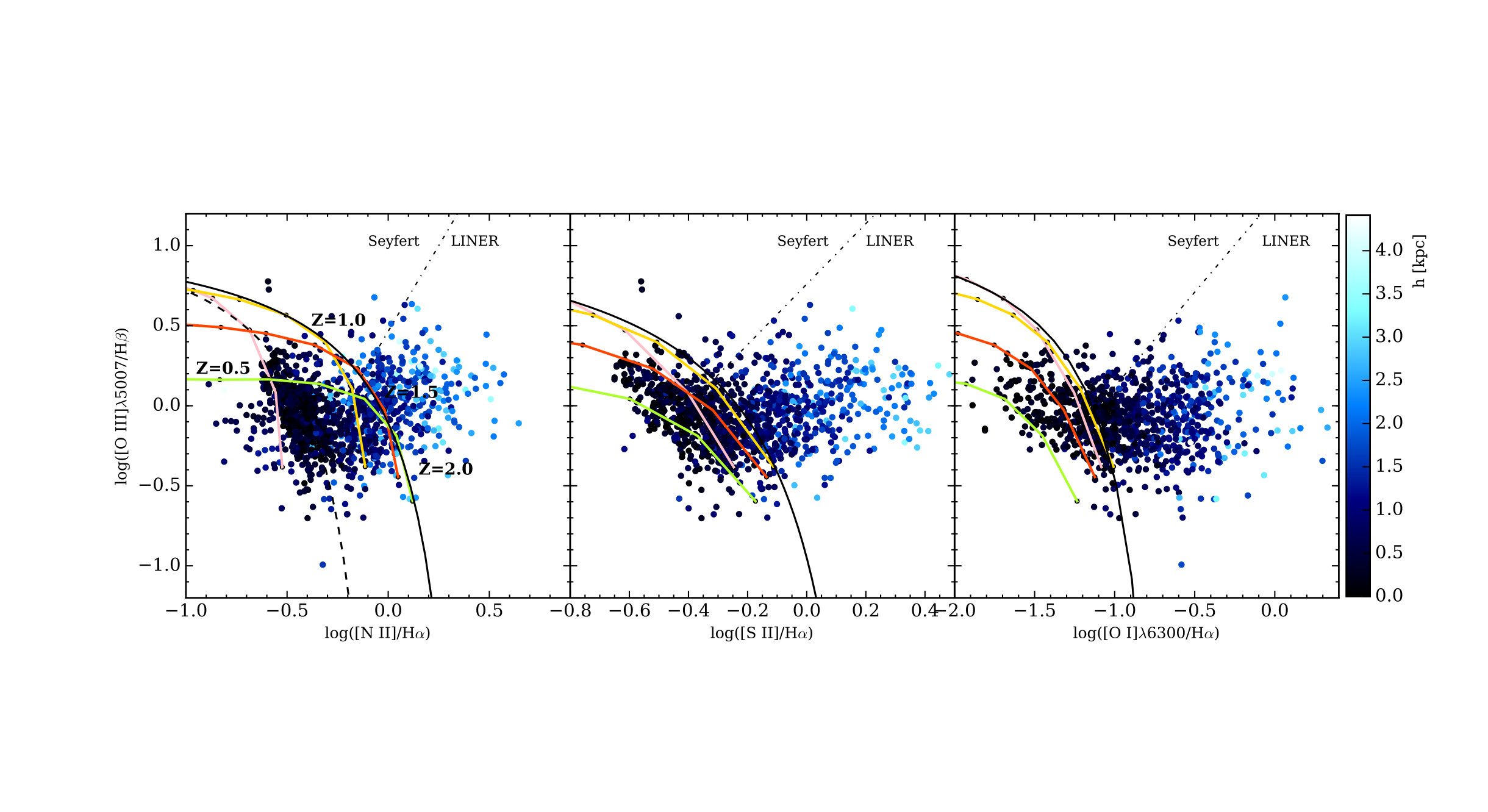 Figure 8
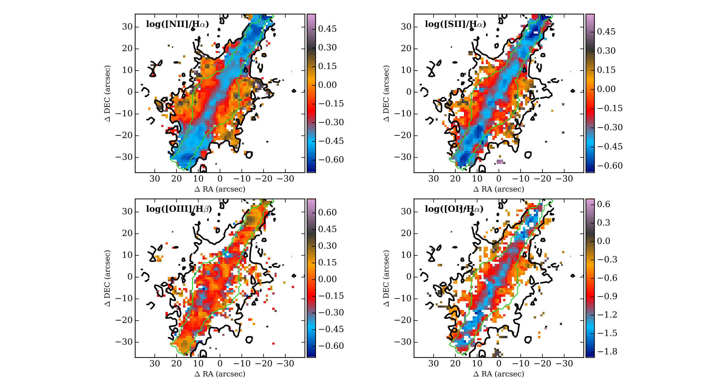 Figure 9
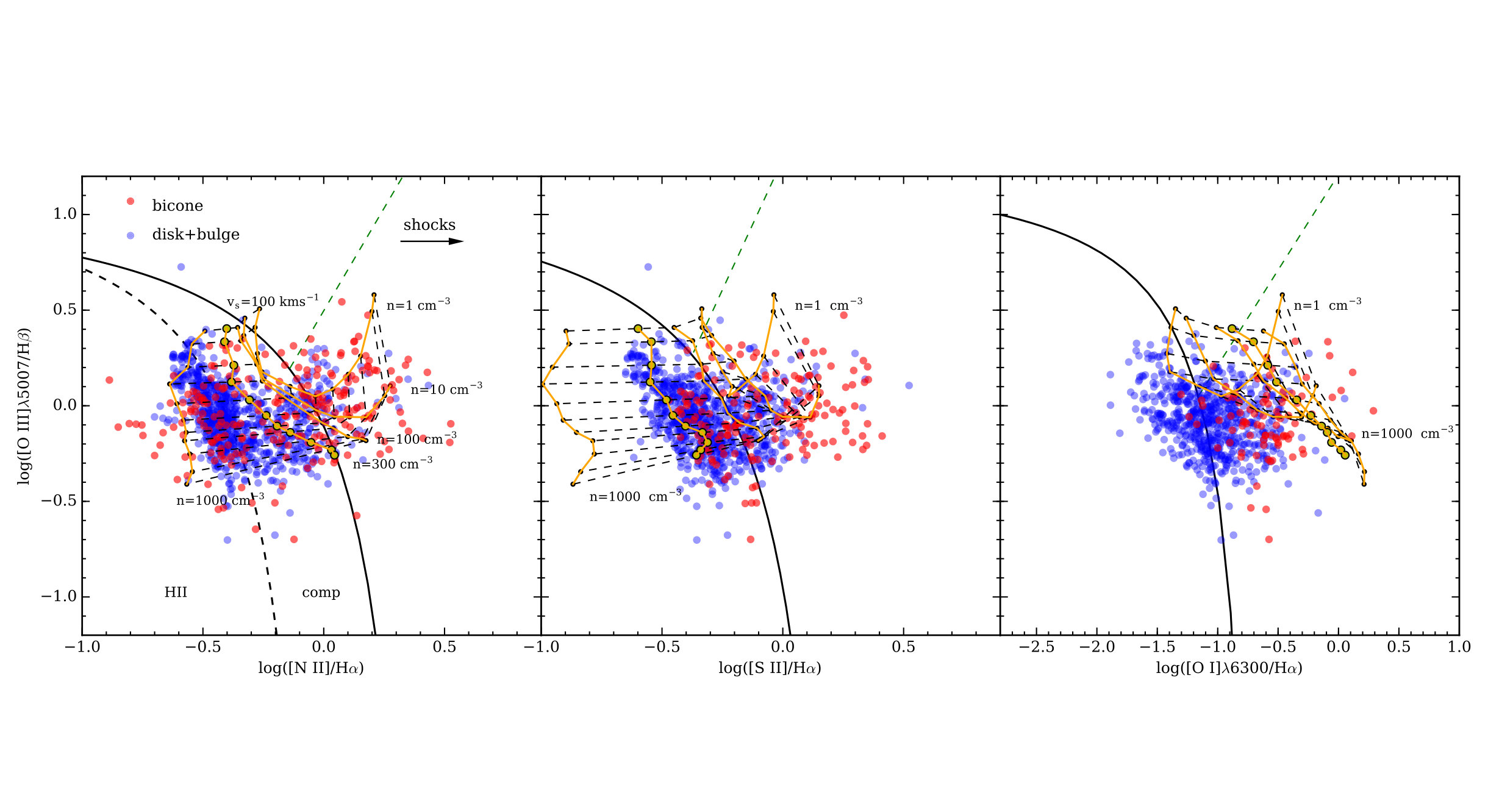 Figure 10
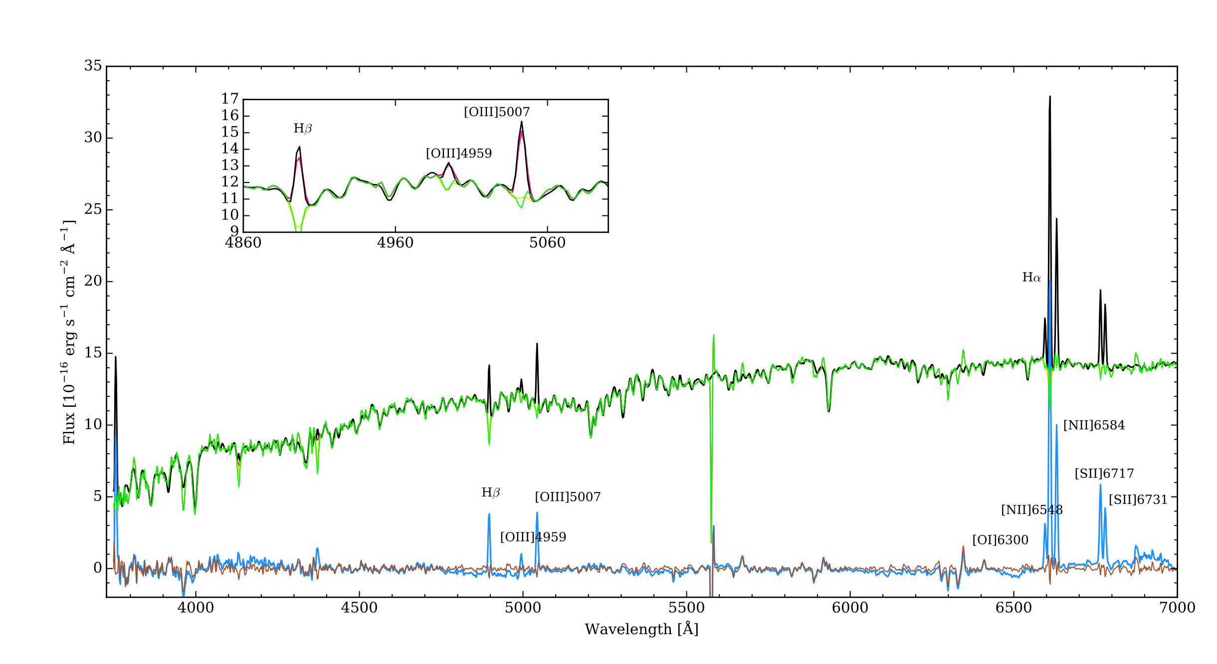 Figure 11
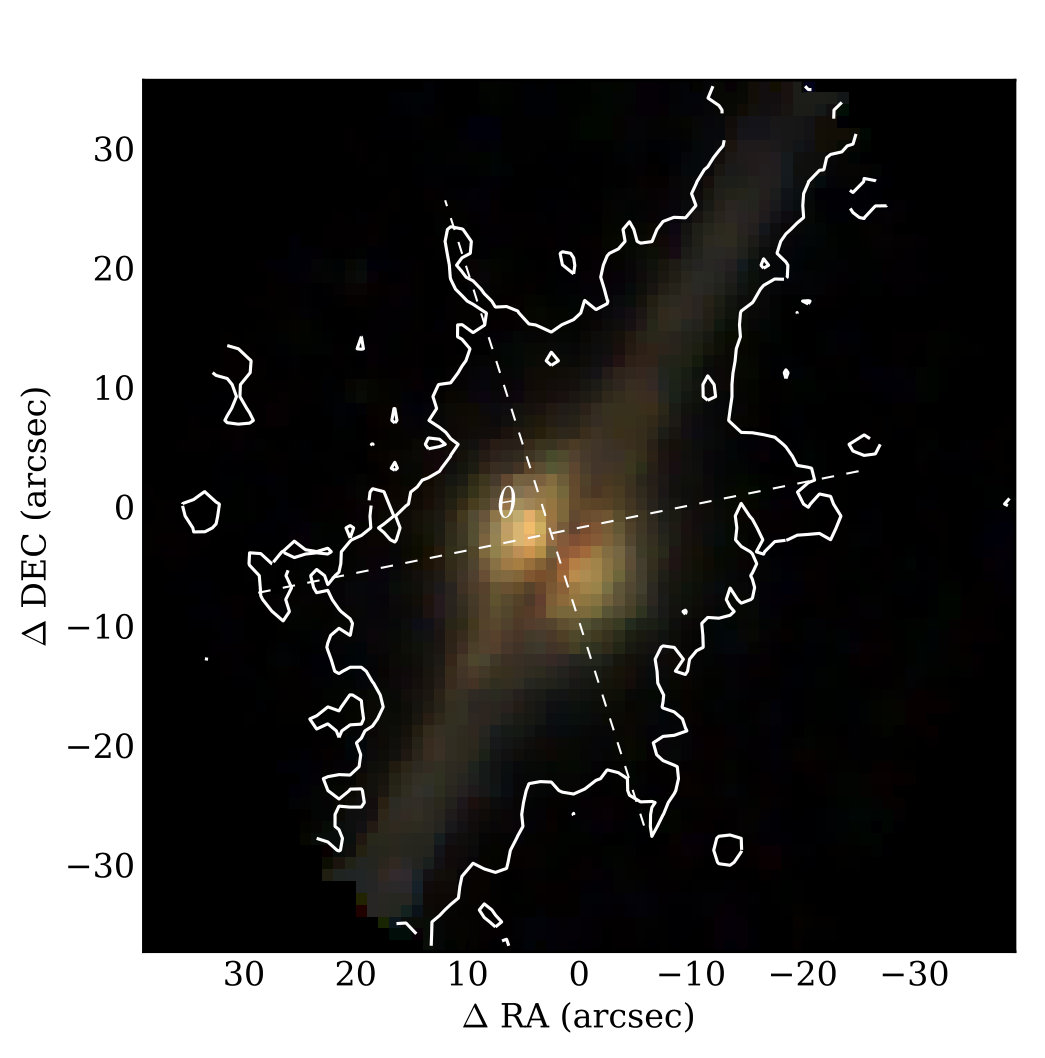 Figure 12
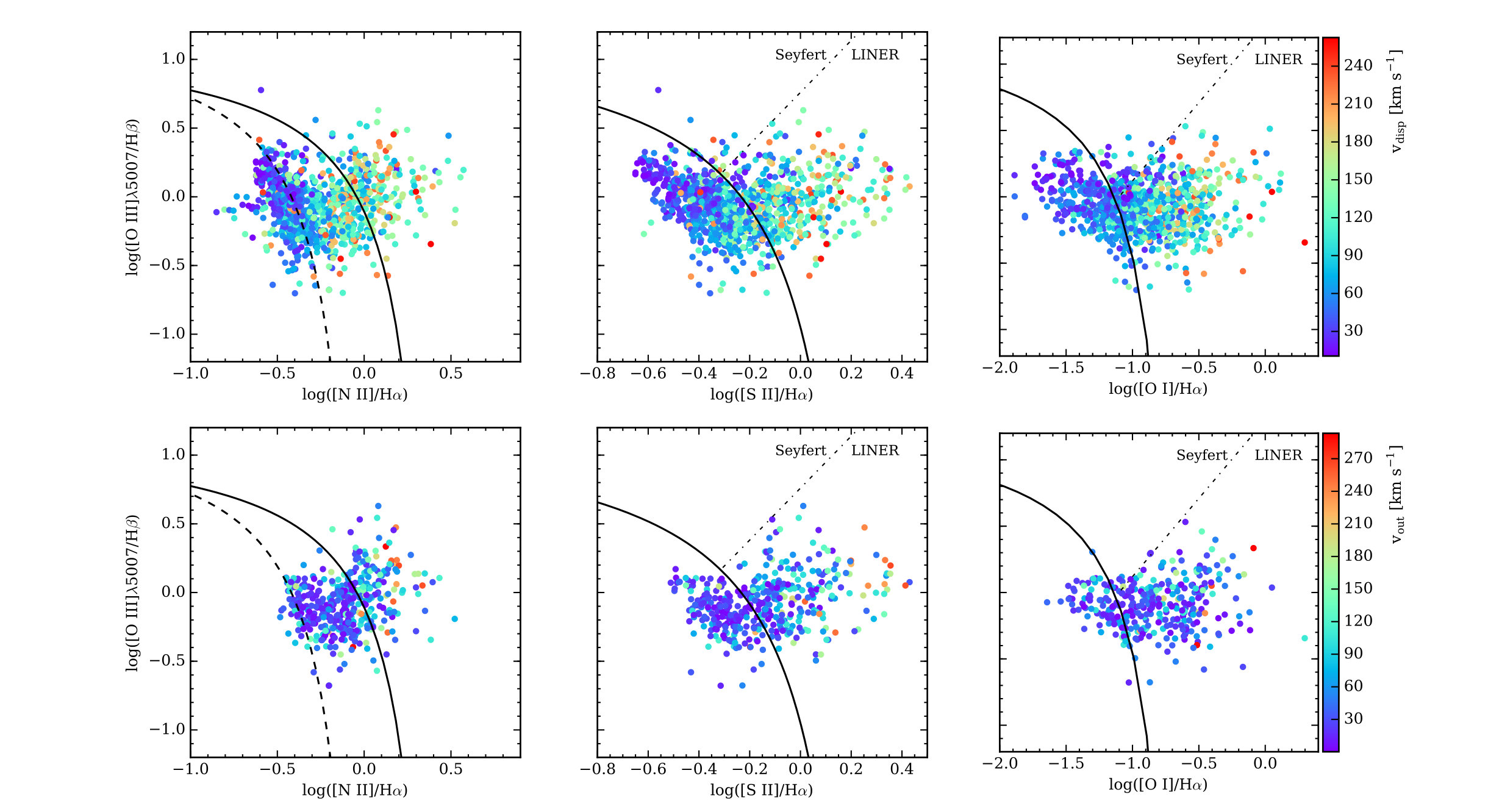 Figure 13
| Parameter | UGC 10043 | References |
|---|---|---|
| Morphology | Sbc | 1 |
| 0.007208 | 1 | |
| (J2000) | 15h48m41.2s | 1 |
| (J2000) | +21d52m09.8s | 1 |
| Distance [Mpc] | 34.995 | 2 |
| [mag] | 32.72 | 2 |
| [deg] | 151.5 | 3 |
| [deg] | 90 | 3 |
| [pc] | 395 | 3 |
| [erg s-1] | 4.51040 | This paper |
| log(M∗/M☉) | 9.79 | This paper |
Peer Reviews
No public reviews on file for this paper yet. If you reviewed it on a platform where reviews are public (OpenReview, ICLR, NeurIPS, ICML), you can paste yours below so the community can read it here.
Videos
No videos yet. Explain this paper in a talk, walkthrough, or lecture? Add one.
Star formation driven galactic winds in UGC 10043
C. López-Cobá1, S. F. Sánchez1, A. V. Moiseev2, D. V. Oparin2, T. BitsakisI. Cruz-González1, C. Morisset1, L. Galbany4,5, J. Bland-Hawthorn6,M. M. Roth7, R.-J. Dettmar8, D. J. Bomans8, Rosa M. González Delgado9, M. Cano-Díaz10,R. A. Marino11, C. Kehrig12, A. Monreal Ibero13 and V. Abril-Melgarejo14
1Instituto de Astronomía, Universidad Nacional Autónoma de México, A. P. 70-264, C.P. 04510, México, D.F., Mexico
2Special Astrophysical Observatory, Russian Academy of Sciences, Nizhnii Arkhyz 369167, Russia
3CONACYT Research Fellow - Instituto de Radioastronomía y Astrofísica, Universidad Nacional Autónoma de México, C.P. 58190, Morelia, Mexico
4Pittsburgh Particle Physics, Astrophysics, and Cosmology Center (PITT PACC), USA.
5Physics and Astronomy Department, University of Pittsburgh, Pittsburgh, PA 15260, USA.
6Sydney Institute for Astronomy, School of Physics, University of Sydney, NSW 2006, Australia
7Leibniz-Institut für Astrophysik Potsdam (AIP), An der Sternwarte 16, D-14482 Potsdam, Germany
8Astronomisches Institut, Ruhr-Universität Bochum, Universitätsstr. 150, D-44801 Bochum, Germany
9 Instituto de Astrofísica de Andalucía (IAA/CSIC), Glorieta de la Astronomía s/n Aptdo. 3004, E-18080 Granada, Spain
10 CONACYT Research Fellow - Instituto de Astronomía, Universidad Nacional Autónoma de México, Apartado Postal 70-264, México D.F., 04510 Mexico
11Department of Physics, Institute for Astronomy, ETH Zrich, CH-8093 Zrich, Switzerland
12Instituto de Astrofísica de Andalucía (CSIC), Glorieta de la Astronomía s/n Aptdo. 3004, 18080, Granada, Spain
13GEPI, Observatoire de Paris, PSL Research University, CNRS, Université Paris-Diderot, Sorbonne Paris Cité, Place Jules Janssen, 92195 Meudon, France
14Departamento de Física, Universidad de los Andes, Cra. 1 No. 18A–10, Edificio Ip, A. A. 4976 Bogotá, Colombia
(Accepted XXX. Received YYY; in original form ZZZ)
Abstract
We study the galactic wind in the edge-on spiral galaxy UGC 10043 with the combination of the CALIFA integral field spectroscopy data, scanning Fabry-Perot interferometry (FPI), and multiband photometry. We detect ionized gas in the extraplanar regions reaching a relatively high distance, up to 4 kpc above the galactic disk. The ionized gas line ratios ([N ii]/H, [S ii]/H and [O i]/H) present an enhancement along the semi minor axis, in contrast with the values found at the disk, where they are compatible with ionization due to H ii-regions. These differences, together with the biconic symmetry of the extra-planar ionized structure, makes UGC 10043 a clear candidate for a galaxy with gas outflows ionizated by shocks. From the comparison of shock models with the observed line ratios, and the kinematics observed from the FPI data, we constrain the physical properties of the observed outflow. The data are compatible with a velocity increase of the gas along the extraplanar distances up to 400 km s*-1* and the preshock density decreasing in the same direction. We also observe a discrepancy in the SFR estimated based on H (0.36 M*☉* yr*-1*) and the estimated with the CIGALE code, being the latter 5 times larger. Nevertheless, this SFR is still not enough to drive the observed galactic wind if we do not take into account the filling factor. We stress that the combination of the three techniques of observation with models is a powerful tool to explore galactic winds in the Local Universe.
keywords:
galaxies: individual: UGC 10043. – galaxies: ISM:. – galaxies: kinematics and dynamics – ISM: jets and outflows.
††pubyear: 2016††pagerange: Star formation driven galactic winds in UGC 10043–Star formation driven galactic winds in UGC 10043
1 Introduction
Galactic winds driven by a combination of supernovae explosions and stellar winds from massive stars have been proposed as a regulating mechanism in the formation and evolution of galaxies (e.g. Silk & Rees, 1998; Springel et al., 2005; Ciardi, 2008). They can also explain the origin of some global properties of galaxies such as (i) the mass metallicity relation (e.g. Tremonti et al., 2004; Finlator & Davé, 2008; Peeples & Shankar, 2011), (ii) the shape of the stellar mass function (e.g. Nakano et al., 1995; Elmegreen, 2001) and (iii) the enrichment of the intergalactic medium with metals (e.g. Aguirre et al., 2001; Oppenheimer & Davé, 2008).
Since the discovery of the central-starburst driven wind in M 82 (Lynds & Sandage, 1963), there have been several works aiming to understand the process that drive galactic winds in active galactic nuclei (AGN), starburst and merging galaxies (Heckman et al., 1990; Rich et al., 2010, 2011; Sturm et al., 2011; Wild et al., 2014). The understanding of feedback processes by outflows plays an important role in the study of galaxy evolution since they may affect strongly the properties of the interestellar medium: i.e. the energy released by star formation (SF, hereafter), and AGN activity into the halo can heat the gas, preventing its cooling and as a consequence suppressing the SF in low-mass galaxies (e.g. Scannapieco et al., 2000; Hopkins et al., 2012). Such processes may have a significant impact on the evolution of the host galaxy by regulating the amount of cold gas available for SF. In addition, the galactic winds can reduce the number of existing dwarf galaxies, since the kinetic energy from supernovae ejects halo gas, thus suppressing the SF (e.g. Dekel & Silk, 1986).
Super-winds are phenomenologically complex since they are comprised of multiple gas phases moving at different velocities (e.g. Bland-Hawthorn, 1995; Heckman et al., 2000; Veilleux et al., 2005; Strickland & Heckman, 2009). The mass released by starburst superwinds can range from tens to thousands of M*☉* yr*-1* with velocities of 100 km s*-1* for the cool component, meanwhile in AGN-driven outflows the velocities exceeds 500 km s*-1*. The mechanism that drives outflows in starbursts is the mechanical energy supplied by supernovae explosions and stellar winds (e.g. Leitherer & Heckman, 1995). It is known that super-winds at high scales are very common in galaxies with SF surface density larger than 0.1 M*⊙* yr*-1* kpc*-2*, both in the local Universe (Dahlem et al., 1998; Lehnert & Heckman, 1996) and at high redshift (Pettini et al., 2001).
Starburst galaxies are commonly observed to host supernovae-driven galactic scale winds (e.g. Heckman et al., 1990; Heckman, 2003). A galactic wind is produced when the kinetic energy ejected by supernovae and stellar winds, produced by massive star formation, is efficiently thermalized. This means that the kinetic energy of the wind is converted into thermal energy via shocks, with a little loss of energy by radiation due to the high temperatures and low densities. The joint effect of supernovae and stellar winds creates a bubble of hot gas (T K) inside the star-forming region with a pressure greater than its environment (e.g. Heckman et al., 1990).
As the bubble expands and sweeps its environment, it quickly turns into a radiative phase. If the environment is stratified, like in the case of galactic disks, the bubble will expand faster in the vertical direction of the pressure gradient. The velocity of this hot gas is expected to be in the range of a few thousands km s*-1* (e.g. Heckman, 2003). Once the bubble reaches a certain scale height, the expansion will accelerate and break into fragments. This will allow the gas to expand freely into the halo and the intergalactic medium follows a bipolar collimated outflow geometry. This is the so-called blow-out phase when the bubble turns into a super-wind. The optical and X-ray emission in the blow-out phase comes from obstacles (clouds, fragmented shells) that are immersed in the gas and are shock-heated by the outflow. This scenario was explained in detail by Heckman et al. (1990).
Huge advantages over classical long slit spectroscopy are obtained by the use of Integral Field Spectroscopy (IFS) to study the spatially resolved properties of galaxies. IFS provides with spatially resolved spectra of a complete Field-of-View (FoV), allowing the study of different components of a galaxy in a simultaneous way. The combination of image and spectroscopy through IFS provides a better understanding of the properties of galaxies. Several works have implemented the use of this technique to study the ionization by shocks and/or outflows of galactic winds (e.g. Rich et al., 2010, 2011, 2014; Ho et al., 2014; Wild et al., 2014; Bik et al., 2015; Mahony et al., 2016). However, to our knowledge, there are no detailed studies of the frequency of outflows in galaxies (see for example Dahlem et al., 1998; Heckman et al., 2000; Heckman, 2003; Ho et al., 2016).
In our current paper, we present the study of the spatially resolved properties of the ionized gas in UGC 10043 based on the data from the Calar-Alto Legacy Integral Field Area (CALIFA) survey (Sánchez et al., 2012), focusing on the analysis of the detected galactic wind. This is a pilot study which ultimate goal is the exploration of the frequency and physical conditions of such outflows in the complete sample of CALIFA. The paper is organized as follows: we present the main properties of UGC 10043 in §2; the data are described in §3, and the conducted analysis in §4. Section 5 describes the analysis of observations with a scanning Fabry-Perot interferometer at the Russian 6-m telescope; while the main results are presented in §6 . Finally, we present the main conclusions and discussion in §7. Throughout the paper, we adopted the standard LCDM cosmology, with parameters 70.4 km s*-1* Mpc*-1*, = 0.268 and = 0.732.
2 Main properties of UGC 10043
UGC 10043 is an edge-on spiral galaxy ( 90°) located at a distance of 35 Mpc (see Table 1). It is found close to MD2004 dwarf, a companion galaxy located 84″to the NW. Matthews & de Grijs (2004) suggested a possible interaction with UGC 10043 which may explain the observed tidal warp in its disk. UGC 10043 presents a very thin disk and a prominent large and bright bulge (Fig. 1). Optical images reveal a very pronounced dust lane along its disk. Matthews & de Grijs (2004), using Hubble Space Telescope (HST) narrow band observations in H [N ii] found evidence of star-formation in its nucleus. They also found H emission perpendicular to the disk following an approximately bi-conic structure resulting from a possible galactic wind. These authors estimate the velocity of the wind in 100 km s*-1* reaching a distance of 3.5 kpc over the disk. Aguirre et al. (2009) mapped UGC 10043 with the VLA. They argued that UGC 10043 is under interaction with MCG 0437035 (located 2.5′to the W; z 0.007398) evidenced by an observed H i bridge between the two galaxies.
3 Data
In our work we are using the IFS observations of UGC10043 from the first and second CALIFA data releases (e.g. Husemann et al., 2013; García-Benito et al., 2015). The CALIFA survey is a recently completed project that comprises three data releases (DR1, DR2 and DR3), the last one delivered in 2016 (Sánchez et al., 2016a). The aim of CALIFA was to obtain spatially resolved spectroscopy of more than 600 galaxies at the Local Universe (0.005 z 0.03) covering a wide range of morphological and stellar masses. The observations cover the optical size of the galaxies up to 2.5 effective radii using the wide-field Integral Field Unit (IFU) Pmas fiber PAcK (PPAK; Kelz et al., 2006) of the Potsdam Multi-Aperture Spectrophotometer instrument (PMAS; Roth et al., 2005). The PPAK fiber bundle consists of 331 fibers of 2.7*′′* diameter each one covering a total hexagonal FoV of with a filling factor of . In order to guarantee a complete coverage of the FoV, three dithering pointings were applied to obtain 993 independent spectra for each object. The final spatial resolution is 1 kpc at the redshift of the sample. This allows to resolve spatially the spectroscopic properties from the most relevant components of the galaxies (H ii regions, bars, spiral arms, bulges). Each galaxy of the CALIFA sample was observed in two different configurations, one of low resolution (V500, R 850) covering the optical range 3750–7500 Å and another one of intermediate resolution (V1200, R 1650) that covers the blue part of the optical range of the spectra 3700–4800 Å. Along this article we use the data of the V500 set-up for UGC 10043.
The data were reduced using version 1.5 of the CALIFA pipeline, whose modifications with respect to the one presented in Sánchez et al. (2012) and Husemann et al. (2013), are described in García-Benito et al. (2015). The procedure comprises the usual steps in reduction of IFS data, as described in Sánchez (2006): bias and dark subtraction, cosmic-ray removal, CCD flat-fielding, spectra tracing and extraction, wavelength and flux calibration, and finally cube reconstruction. The final product of the data reduction is a regular-grid data-cube, with and coordinates indicating the right ascension and declination of the target and a common step in wavelength. The CALIFA pipeline also provides with the propagated error cube, a proper mask cube of bad pixels, and a prescription of how to handle the errors when performing spatial binning (due to covariance between adjacent pixels after image reconstruction).
These data were complemented with multi-band, aperture matched, photometry extracted from the Galaxy Evolution Explorer (GALEX; Martin et al., 2005), Sloan Digital Sky Survey (SDSS; York et al., 2000), and Wide-Field Infrared Survey Explorer (WISE; Wright et al., 2010) surveys, extracted following the procedures described in Bitsakis et al. (in prep.). To estimate the physical properties of this galaxy, these authors provided a spectral energy distribution (SED) modelling, using CIGALE (Noll et al., 2009).
We also use Fabry-Pérot Interferometer (FPI) observations obtained at the prime focus of the 6-m telescope of Special Astrophysical Observatory Russian Academy of Sciences (SAO RAS) in 2014 May 24/25. The scanning FPI was mounted inside the SCORPIO-2 multi-mode focal reducer (Afanasiev & Moiseev, 2011). The operating spectral range around the [N ii] emission line was cut by a narrow bandpass filter with a Å bandwidth. The interferometer provides a free spectral range between the neighbouring interference orders Å with a FWHM of the instrumental profile Å (R3860). During the scanning process, we have consecutively obtained 40 interferograms, each of 1800 s exposure, at different distances between the FPI plates, under seeing conditions of ″. The FoV was with a sampling of per pixel. The data were reduced using algorithms and programs described by Moiseev & Egorov (2008) and Moiseev (2015). Thus, each spaxel in the reduced data cube contains a 40-channel spectrum.
4 Analysis
4.1 Continuum Subtraction
To study the properties of the ionized gas we need to uncouple the continuum from each spectra of the data-cube. There are several routines focused in the analysis of the stellar populations (e.g. STARLIGHT, pPXF, Cid Fernandes et al., 2011a; Cappellari & Emsellem, 2004). Here we adopted Pipe3D, a pipeline developed to analyse IFS data-cubes (Sánchez et al., 2016c, S16 hereafter) using the fitting package FIT3D (Sánchez et al., 2016b, S15 hereafter).
Generally the continuum spectra show a wide range of signal to noise ratios (SN) that are higher in the central regions and gradually decreasing outward from the galactic centre. From simulations tested in S15, we observed that a minimum SN is required in each spectrum to obtain an accurate model of the continuum and therefore to derive the properties of the ionized gas. In order to increase the SN in each spectrum we perform a spatial binning of the cube in the optical range selecting as a goal value a SN 50. In Fig. 3 we show the result of this tessellation procedure. This tessellation has one advantage compared to other methods, such as the Voronoi one (Cappellari & Copin, 2003), that the performed segmentation follows the morphology of the galaxy and at the same time increases the SN, as described in S16.
Once the tessellation is performed, all the spectra within each spatial bin are co-added and treated as a single spectrum. Then, we derive a stellar population model for each of those spectra by performing a multi Synthetic Stellar Population (SSP) fit. Finally, we recover a model of the stellar continuum for each spaxel by re-scaling the model within each spatial bin to the continuum flux intensity in the corresponding spaxel. The stellar population model is then subtracted to create a pure gas data-cube comprising only the ionized emission lines (also including the noise and the residuals of the stellar population modelling). The strongest emission lines within the considered wavelength range are fitted spaxel by spaxel for the pure gas cube, adopting a single Gaussian function for each considered emission line. By doing so, we derive their corresponding flux intensity and the propagated errors. Finally, we can extract a set of 2D maps comprising the spatial distribution of the flux intensities for each analysed emission line. In Figure 2, we show the results of the fitting procedure for one single spectrum to illustrate the full process.
4.2 Ionized gas emission
In Figure 4 we show the intensity maps for the emission lines H, [N ii]6584, [O iii]5007, H, [S ii]6731,6716 and [O i]6300 with a cut in SN . This cut decreases the number of useful spaxels in each map but not significantly. From these maps we observe that most of the contribution to the ionized gas is located in a narrow region associated to the disk. There is another evident component of ionized gas that is uncoupled from the disk, located in the extraplanar regions. This extraplanar emission of ionized gas extends perpendicular to the disk and is clearly visible in H, [S ii], and [N ii] maps.
4.3 Spatial variation of the emission line ratios
The ionization stage of a photoionized nebula is mainly determined by three parameters: the ionization parameter 111, where is the number of ionizing photons emitted by the source per second, is the distance between the source and the nebula, is the electron density and the light speed., the hardness of the ionizing radiation (depending on the effective temperature and metallicity of the star, or the age and metallicity of the cluster, or the characteristics of the AGN), and the optical depth at the Lyman continuum (matter bounded regions having higher ionization stages). Furthermore, the ionization stage of shocked regions is determined by the characteristics of the shock (speed, magnetic field, densities).
The emission line ratios involving the strong lines [N ii], [S ii], [O iii], [O i] and the Balmer lines (H and H) have been proposed as a method to classify between regions ionized by AGN and softer ionizing sources as H ii regions (see Veilleux & Osterbrock, 1987). With the use of IFS, we are able to spatially resolve the location of different ionization sources by analysing their line ratios. As a first step, we study the spatial distribution of the strongest emission line ratios and investigate if there is any correspondence with the population properties.
Figure 5 shows line ratio maps of [N ii]/H, [S ii]/H, [O iii]/H and [O i]/H. The line ratios [N ii]/H and [O iii]/H are insensitive to dust extinction, as the emission lines are close in wavelength. The other emission line ratios are also close in wavelength, excluding [O i]/H. We include the [O i]/H emission line in our analysis despite the weakness of [O i], because it is a good discriminator between photoionization by hard ionizing power-law sources and OB stars, and also because it is a good tracer of shock excitation (e.g. Rich et al., 2010; Farage et al., 2010).
A first inspection of the line ratio maps reveals a remarkable increase in all line ratios from the disk toward the extraplanar regions, being more evident in the [N ii]/H and [S ii]/H maps. If we assume that H traces the extension of the disk as seen in Fig. 4, then we observe that the line ratios change starts at the edge of the disk.
The [O iii]/H line ratio covers a smaller area due to our cut in SN in H, since H is 3 times weaker than H. On the other hand, the [O i]/H map is less populated because [O i] is a weak line compared to [N ii] and [S ii]. The line ratios at the disk region in the [N ii]/H map are consistent with the maximum ratio (log [N ii]/H ) observed in star forming regions (e.g. Kauffmann et al., 2003). The [O iii]/H line ratio is more or less constant throughout the galaxy. The increase in the line ratios [N ii]/H, [S ii]/H and [O i]/H far away from the galactic disk has also been observed in the case of extraplanar diffuse ionized gas (DIG) in edge-on galaxies, in which the ionization at kiloparsec scales is produced by hot old stars in the halo with electron densities in the extraplanar region lower than 10*-1* cm*-3* (e.g. Tüllmann et al., 2000; Flores-Fajardo et al., 2011).
4.4 Diagnostic Diagrams
In order to understand changes in line ratios across the field of view, we explore the so-called diagnostic diagrams. Baldwin, Phillips and Terlevich proposed a diagram that compares the line intensity ratios [O iii]/H versus [N ii]/H (known as the BPT diagram, Baldwin et al., 1981), to separate the emission from soft ionizing sources, like H ii regions, and objects with a higher ionizing power, as AGNs. However, these line ratios are less accurate to distinguish among objects of low ionization, like weak AGNs, excitation by shocks, planetary nebulae and ionization by post–AGB stars (e.g. Binette et al., 1994; Morisset & Georgiev, 2009; Binette et al., 2009; Cid Fernandes et al., 2011b; Kehrig et al., 2012; Singh et al., 2013). Subsequently, Veilleux & Osterbrock (1987) extended this scheme incorporating the diagnostic diagrams for the [S ii]/H and [O i]6300/H line ratios. Both line ratios are sensitive to ionization by shocks, being [O i]/H the most sensitive.
Different demarcation lines have been proposed for these three diagnostic diagrams. The most frequently used ones are those by Kewley et al. (2001) and Kauffmann et al. (2003). The most recent ones Richardson et al. (2014) and Richardson et al. (2016) are shown in Fig. 6. The Kewley et al. (2001) curve was determined by means of photoionization models. It is the maximum envelope that can be reached if the ionization is produced by a single or multiple bursts of star formation. The Kauffmann et al. (2003) curve was obtained empirically from galaxies of the Sloan Digital Sky Survey (SDSS). It traces the approximate upper limit of the sequence of the SF region in this diagram. The two curves are frequently used to distinguish from SF regions (below the Kauffmann curve) and AGNs (above the Kewley curve). The intermediate region between the two curves is usually interpreted as a composite zone due to a combination of different ionization sources. However, this can also be populated by ionization due to starburst galaxies with continuous SF (e.g. Kewley et al., 2001), post-AGB stars (see Cid Fernandes et al., 2011b; Papaderos et al., 2013; Sánchez et al., 2014), shock ionization (e.g. Rich et al., 2010; Ho et al., 2014; Alatalo et al., 2016), or even classical H ii regions in evolved areas of galaxies (e.g. Oey & Kennicutt, 1993; Sánchez et al., 2015).
In Fig. 6, we show the classical BPT diagram for the individual spaxels. According to the spatial distribution of line ratios observed in Fig. 5, our interpretation is that the extraplanar emission is not likely due to photoionization by young stars. These points are spread over the region dominated by star formation towards the region classically dominated by AGN. So far there is no evidence of the presence of an AGN in this galaxy, which is also consistent with its small mass and bulge. Therefore, we discard AGN as the possible ionization source for UGC 10043.
Due to the shape and geometry of the extraplanar emission, the distribution of line ratios from the star forming region towards the intermediate AGN area, and the lack of evidence of an AGN, we consider that the extraplanar emission is related to shock ionization induced by a galactic wind created by a central SF event. From Figs. 4 and 5 we observe a symmetrical distribution of the extraplanar gas with respect to the galactic disk. If we assume that the burst of SF was in the nuclear region of the galaxy, and assuming an ideal biconical distribution of the ionized gas (e.g. Heckman et al., 1990) we can trace the limit of the outflowing region based on the distribution of emission lines. The expected conic structure was already shown in Fig. 1
We will try to confirm the suspicion of shock ionization by comparing the properties of the emission lines with the predictions by photoionization and shock models.
4.5 Photoionionization models
In Fig. 7 we compare the observed line ratios with the predicted ones by photoionization models along the diagnostic diagrams described in previous sections: [N ii]/H, [S ii]/H, [O i]/H versus [O iii]/H. The points are color–coded by their distance from the galaxy disk. The three panels include the predicted values from the MAPPINGS-III photoionization models (Allen et al., 2008), for continuous SF bursts, and using the PEGASE 222http://www2.iap.fr/pegase/pegasehr/ synthetic stellar library, as described by Dopita et al. (2000) and Kewley et al. (2001). Each line corresponds to a different stellar abundance (ZZ*☉* = 0.5, 1, 1.5 and 2). For each of them the ionization changes from high-ionization (top-left) to low-ionization (bottom-right). In all cases an average electron density of cm*-3* is assumed. We would like to stress here that the farther a region is located from the disk the stronger the ionization it presents (out to 4 kpc).
Thus using a continuous starburst photoionization model we can reproduce the line ratios that lie below the Kewley et al. (2001) curves, whose spatial location is in the disk of the galaxy. These regions are most probably associated with star forming regions as we suspected, nevertheless ionization by shocks cover part of the star forming region, as we will see later. Furthermore, there are several line ratios in the diagnostic diagrams that are not covered within the parameters space of these photoionization models.
4.6 Shock models
In Figs. 6 and 7, we described two main components in the ionization mechanism, one produced by young stars at the disk and an extraplanar emission that is not reproduced by the analysed photoionization models. Most probably, this extraplanar ionization can be produced by radiative shocks during the warm phase (T 104 K) of a galactic wind as described above. The observed ionized gas can be located over the walls of the conic structure or in filamentary structures from the nuclear region. Shock ionization can be located in the diagnostic diagrams in areas distributed from the classical location of H ii regions towards areas where AGN ionization is dominant (e.g. Davies et al., 2014).
The signatures of shocks can be seen as double peaks or broad components in the velocity dispersion profiles due to the different kinematic components along the line of sight and the morphology of the ionized gas. Due to the low spectral resolution of the CALIFA data, we are not able to separate the different kinematic components in the velocity dispersion profiles, and therefore uncouple and analyse them separately. At the wavelength of H the instrumental resolution of our data is 116 km s*-1*, which exceeds the typical velocity dispersion of H ii regions ( 100 km s*-1*, Yang et al. (1996); Moiseev et al. (2015)). Thus, it is not enough to distinguish different kinematic components of the order expected by shocks (e.g. Lehnert & Heckman, 1996). Moreover, even FPI data taken with a significant higher spectral resolution ( 33 km s*-1*) did not resolve a multicomponent structure of the [N ii] emission line profile, and only line broadening and asymmetric profiles were observed (see Sec. 5). Broadening profiles in regions outside the galactic disk has also observed in starburst–driven galactic winds (e.g. Westmoquette et al., 2010). The presence of broad line profiles suggests that complex kinematics components could exist that are still unresolved at the spectral resolution of our FP data. Therefore, we need to compare the observed line ratios with the predictions from shock ionization models to determine if the ionization is driven by shocks, and if so, derive its physical conditions.
We adopt grids of shock models from the MAPPINGS III library of fast radiative shock models (Dopita & Sutherland, 1995, 1996; Dopita et al., 2005; Allen et al., 2008). We selected a shock velocity () range of 100 to 400 km s*-1* in intervals of 25 km s*-1* and a transverse magnetic field flux density of 5 G. For the gas component, we explored a range including both solar and supra-solar abundances, and pre-shock densities of 1, 10, 100 and 1000 cm*-3*, respectively. In Fig. 8, we plot the diagnostic diagrams for the different line ratios explored in Fig. 5, together with the values predicted by the adopted shock models without precursor. In this plot we have added a different demarcation from the classical LINER–AGN. The new demarcation is a bisector line which separates the ionization by shocks from AGN estimated from two fiducial clear objects of this kind of ionization using IFS data according to Sharp & Bland-Hawthorn (2010). In addition to the shown models, we have explored many different combinations of magnetic fields and pre-shock densities, along with the possible presence of a precursor. However, none of them reproduce the observed line ratios in the three diagrams simultaneously, as well as the models that are presented in Fig. 8.
The shock models in the [N ii]/H and [S ii]/H diagrams cover areas frequently associated with continuous SF (e.g. Kewley et al., 2001; Sánchez et al., 2015) and low ionization nuclear emission–line regions (LINER) (e.g. Gomes et al., 2016). We observe that the majority of the points above the Kewley curves are located at the right side of the bisector line towards the locus of shock excitation and therefore in the extraplanar region. For these diagrams we make a distinction between the regions that lie in the disk and those in the bi-cones according to our demarcation shown in Fig 4. There is ionization spatially located at the bi-cones below the Kauffmann curve, most probably due to the low shock velocities components in the emission lines. Our selected shock model describes pretty well the line ratios for the outflow zone in the [N ii]/H and [S ii]/H diagrams and covers partially the observed line ratios for [O i]/H. The shock models describe the outflow region for a wind with a pre-shock density decreasing toward larger extraplanar distances with an increase of velocity up to 400 km s*-1* in the same direction.
5 Fabry-Pérot Interferometer data on gas kinematics
5.1 Kinematic maps
The Fabry-Pérot Interferometer data provide information about ionized gas kinematics with velocity resolution four times better than that of the PPAK/V500 data, in a significantly larger field-of-view, but with a shallower depth. The observed profiles of the [N ii] line were fitted with a Voigt function, which is a convolution of a Lorentzian and a Gaussian function corresponding to the FPI instrumental profile and broadening of observed emission lines, respectively (Moiseev & Egorov, 2008). The emission-line spectrum is very well described by a single-component Voigt profile without double or multi-components structures. Fig. 9 shows two-dimensional maps derived from the fitting process, including the intensity map of [N ii]6584, its line-of-sight velocity field, and its line-of-sight velocity dispersion () determined by broadening of emission line. The maps are masked using a SN threshold in the flux intensity. In the first panel we also plot the spectrum of key regions in the galaxy, showing two regions within the disk, and other two in the areas of maximum velocity dispersion located along the semi-minor axis within the outflow cone. We observe broad and asymmetric profiles without a remarkable separation of double or multiple components, typically found in galactic winds driven by SF in these two latter regions (e.g. van Eymeren et al., 2009).
At the outer parts of the disk we observe a low velocity dispersion (10-40 km s*-1*), which is the typical value for giant H ii regions in galaxies (e.g. Moiseev et al., 2015). While in the wind bi-cones exceeds 100 km s*-1*, increasing towards larger distances from the galactic disk, reaching vales km s*-1* probably because at higher distances from the disk the density of the ISM is lower. These values of the velocity dispersion are roughly consistent with the shock models described before, for which the expected velocities are expected to be lower than 400 km s*-1* .
The FPI map shows that the circular rotation makes a mayor contribution to the observed line-of-site velocities even in the galactic wind region. This picture is typical for edge-on disk galaxies with a relatively moderate outflow (e.g., NGC 4460, Oparin & Moiseev, 2015). The mean rotation curve was subtracted from the observed velocity field with the aim to remove the regular velocity gradient. We use a model of a transparent rotating cylinder that provides a good approximation of velocity fields in edge-on rotating disk galaxies as described in detail in (Moiseev, 2015). In short, the rotation curve was calculated from averaging points across the galaxy major axis, the amplitude of ionized gas rotation in UGC 10043 reaches 150 km s*-1*. The mean rotation curve was extrapolated outside the galactic mid-plane to create a model of galactic rotation. The residual line-of-sight velocities after the circular rotation subtraction are shown in the last panel of Fig. 9. This map reveals a dozen “spots” inside the outflow bi-cones with typical residual velocities km s*-1*. The symmetrical distribution of the residuals relative to the major axis implies that we are able to observe real regular deviations of line-of sight-velocities from the circular rotation produced by the wind outflow.
5.2 Outflow velocities
We translated the observed line-of-sight residual velocities into wind outflow velocities in the frameworks of a simple geometrical model presented by Oparin & Moiseev (2015). The wind nebulae is described by frustum rotating bi-cones. The matter ejected from the galactic circumnuclear region forms a single large shell. While the inner hot gas here is transparent at visible wavelengths, the walls of the bi-cones could be observed in optical recombination lines. From the velocity dispersion map shown in Fig. 9 it is clear that the shocked ionized gas follows a conical distribution, with a low velocity dispersion at the central regions( 100 km s*-1*), and at the edges of the cone. Following this kinematic structure we estimate the opening angle as (as marked in Fig. 9), traced by eye at the location of the maximum gradient in the velocity dispersion. This aperture angle is smaller than the one one estimated from the morphology of the ionized gas emission based on the CALIFA data. This is most probably because the former traces the location of the observed change in the velocity dispersion, which the latter traces the largest extension of the ionized gas. We note that according to observations of winds in other galaxies, like M 82, cone walls visible in the optical are not homogeneous but consist of several emission filaments.
Under this assumption, the observed gas belongs to the cone walls and moves along them out of the galactic disk with an outflow velocity . For an edge-on galaxy the positive velocities correspond to the gas on the walls closest to us, while the matter with negative velocities moves along the farthest wall. According to the formula in Oparin & Moiseev (2015) for the galactic inclination :
[TABLE]
where is the residual line-of-sight velocity after subtracting the pure circular rotation, is the azimuth angle relative to the axis of the cone. With this equation several regions with a large amplitude of translated into fast moving filaments with 100–250 km s*-1*, while the velocities of the neighbouring points are significantly smaller. These de-projected outflow velocities are in the range of those found in the surface of bipolar structures (e.g. Heckman et al., 1990; Heckman, 2003). Therefore, we confirm the measurements of the wind velocities are consistent with shocks models, as in the case of the distribution of (see §. 5.1).
5.3 Line ratios versus kinematics
As it was shown before, the kinematic parameters of the extraplanar outflow derived from FPI observations, km s*-1*, and km s*-1*, are in a good agreement with our estimation of shock velocities obtained from the shock models (100–400 km s*-1*). It is interesting to compare directly spaxel-to-spaxel both quantities with emission line ratios on BPT diagrams. We re-binned the FPI maps to the CALIFA pixel scale to make this comparison.
The results are presented in Figs. 10 and 11. Figure 10 show the same diagnostic diagrams shown in Fig. 7 and 8, with the values labelled according to the velocity and velocity dispersion of the FPI data. The diagrams revealed that the points having high outflow velocity and/or velocity dispersion are indeed located in the region corresponded to shock excitation of forbidden lines. This relation is more clear in the case of velocity dispersion, but the spread of points with the same is too high for an unambiguous conclusion. The latter might be related to limitations of our very simple geometrical model, as well as with the fact that the points on the diagrams do not correspond to these independent points in the volume. Indeed, in each pixel we observe integral values along the line-of-sight for both the lines intensities and their velocities.
We compare the four main emission line ratios used throughout the paper with the corresponding velocity dispersion in Fig. 11. This figure shows a clear correlation between the velocity dispersion and the line ratios indicating shock excitation ([N ii]/H, [S ii]/H, [O i]/H). While for the [O iii]/H ratio the dependence disappears, because the link between this line ratio and the type of ionizing source is ambiguous for [O iii]/H. The extraplanar distance reached in these maps is lower than that shown in Fig. 7 due to the limited depth of the FPI data. Similar plots with a positive correlation between the velocity dispersion and BPT line ratios have been considered by different authors that used 3D-spectroscopic technique in studies of SF galaxies and ULIRGs (cf. Monreal-Ibero et al., 2006, 2010; Ho et al., 2014; Martín-Fernández et al., 2016, and references therein). In the case of UGC 10043 the correlations shown on the Fig. 10, and the trend with galactocentric distances, give additional arguments in favour of shock-wave origin of the emission lines emission in wind nebulae.
6 Results
Based on our emission maps and the morphology of the outflow we find that most probably the wind in UGC 10043 is found during the blow–out phase where the bubble has broken. At this stage the wind is free to expand in the intergalactic medium carrying metals, mass and momentum. The [N ii], [S ii] and H intensity maps reveal a gas flux following a hourglass shape, originated from the centre of the galaxy where the SF is more intense. Adopting a symmetric bi-conic geometry, and following the ionized gas distribution from the maps, we determined morphologically the aperture angle of the cones in 80 and kinematically in 45. Here we describe the physical conditions of this outflow.
6.1 Properties of the ionized gas
6.1.1 Electron Density
From the emission of the Sulfur doublet [S ii]6716, 6731 we determine the electron density across the galaxy (see Osterbrock, 1989), by solving the equation (McCall, 1984):
[TABLE]
where is the density parameter defined as 10 and is the electron temperature in units of 104 K. Here we adopted an electron temperature of 10,000 K for the optical emission region in shocks, following Heckman et al. (1990). Fig. 12 shows the spatial distribution of the intensities in the Sulfur ratio together the electron density derived from Ec. 2. An electron density 200 cm*-3* is predominant in the whole galaxy, increasing slightly toward the cones region. These electron densities are clearly higher than the expected in DIGs. Thus, even in the presence of a DIG, the extraplanar emission is most probably dominated by shocks.
6.1.2 H Luminosity
Based on the H flux intensity map, we determine the luminosity from those regions where the ionization is due to OB stars, after correcting the flux for dust extinction effects (estimated from the observed H/H line ratio), and taking into account the cosmological distance. We assume the extinction curve of Cardelli et al. (1989) with the specific attenuation coefficient of 3.1 (similar to the Milky Way one). We assumed an intrinsic line ratio of H/H= 2.86 corresponding to Case B recombination (Osterbrock, 1989), for 10,000 K and 100 cm*-3*. Adopting a cosmological distance for this galaxy of 35 Mpc, we obtain a total H luminosity of (4.47 0.02) 1040 erg s*-1* (see Table 1).
6.1.3 Star Formation Rate
The H luminosity is frequently used as an indicator of the Star Formation Rate (SFR) in galaxies (Kennicutt, 1998). After correcting H emission by dust extinction it is possible to determine the SFR for those regions where the ionization is produced by young stars (e.g. Catalán-Torrecilla et al., 2015). If we assume that the regions lying below the Kauffmann curve in the BPT diagram are star forming, and apply Kennicutt relation, we can estimate a global SFR = M*☉* yr*-1*.
We also estimate the SFR using the CIGALE code (Noll et al., 2009). This code accounts on the global energy balance between the energy absorbed by dust in the UV-optical bands and the re-emitted one in the infrared, and models the spectral energy distributions (SEDs) as described before. During this procedure the stellar emission, and both the absorption and emission by dust are taken into account. The code derives the likelihoods of the current stellar mass and SFR, from the set of fitted SEDs. We estimate a SFR of (1.56 0.23) M*☉* yr*-1*. This value is times larger than our previous estimates. This discrepancy in the SFRs is not surprising. The high inclination of UGC 10043 only allows us to observe the emission of the ionized gas located at the most outer parts of the disk. Thus, the observed H may not be representative for the overall galaxy emission. The contribution of the ionized gas in the most inner regions are opaque due to the high extinction of the galactic disk. The CIGALE code takes into account both the dust absorption and its re-emission in the infrared, so we expect a higher SFR value. In the following sections we will explore the possibility that these SFR estimates are strong enough to drive the observed outflow within the range of the estimated physical parameters.
6.1.4 Energetic conditions
Our results indicate that most probably the ionization is due to shocks by galactic winds driven by recent star formation. We would like to explore the energy injection due to the SFR. To do this we follow previous works by Heckman et al. (1990) and Wild et al. (2014).
Our data allow us to determine the rate at which the wind carries momentum and energy. The density in the medium, (i.e. the pre-shock density ) at which the wind is propagated can be determined through the electron density () derived before, if we assume equilibrium between the post–shocked gas and the warm gas at T 104 K:
[TABLE]
where is the shock velocity. The thermal pressure (Pgas) of the clouds where the line ratios are emitted is given by:
[TABLE]
where is the proton mass and = 1.36 accounts for an assumed 10 Helium number fraction and we adopt an electron density cm*-3* (see Sec. 6.1.1). The momentum flux can be expressed as:
[TABLE]
where P is the pressure of the wind at distance . From Fig. 7 we estimate a maximum distance of 4 kpc. The solid angle is determined for both apertures angles of the cones 45 80.
In the blow–out phase of a galactic wind the source of pressure can be located in filaments originated in the nuclear region or in the external walls of the wind. If the ionized gas is emitted in filaments, or in clouds then the pressure of the wind is comparable to the pressure of the gas, Pwind = Pgas. If the ionized gas is located in the walls then the pressure of the wind is larger than that of the gas, Pwind = P, where is the perpendicular component of the velocity over the walls. From Fig. 1, .
Knowing the velocity of the super-wind we could estimate the energy rate:
[TABLE]
The velocity of the wind fluid that drives the large scale outflow is poorly constrained in starburst–driven winds. This wind is very hot and tenuous and is quite hard to detect. Super-wind models predict velocities in the range of 1000–3000 km s*-1* (Hopkins et al., 2013). Therefore, if the ionized gas lies in filaments (Pwind = Pgas ), then we estimate the energy carried out by the wind within this velocity range as:
[TABLE]
[TABLE]
On the other hand, if the ionized gas is located in the walls of the cone, then the energy of the wind is within the range:
[TABLE]
[TABLE]
Once estimated the energy of the wind, we can compare it with the injection rates predicted by supernovae and stellar winds due to SF. This has been estimated using synthesis models of stellar populations from young stars (Veilleux et al., 2005):
[TABLE]
While if we use the SFR estimated with CIGALE, then we obtain erg s*-1*. We note that in the case of the gas located in the walls the energy of the wind is larger than that due to SF.
6.1.5 The filling factor
For the previous calculations we have considered that the whole volume of the cones is occupied by gas. The ionized gas fraction contained inside the conical structure is parametrized by the filling factor . According to Heckman et al. (2000) this factor is 10*-3*. The filling factor affects directly in the derivation of the electron density and therefore the energy of the wind, which has a linear dependence on the electron density. This means that the real energy of the wind must decrease up to a factor of 3 orders of magnitude. This is in concordance with the hypothesis of the ionized gas in the walls, in which the energy from SF is up to 10*-2* times the energy of the wind. Due to the uncertainty in we can only obtain an upper limit in the energy of the wind, and we are not able to discard clumpiness or a filamentary structure of the ionized gas.
7 Conclusions
We used the unique capabilities of the CALIFA survey to study the emission of the ionized gas in the edge on galaxy UGC 10043. We detect the presence of a possibly bi-conical extraplanar emission of ionized gas that reaches distances up to 4 kpc over the galaxy disk. We favour, that this extraplanar emission is most probably produced by a galactic wind driven by a weak nuclear starburst, consistent with a low SFR = M*☉* yr*-1* as measured with H.
Based on shock models, we find that our data are better described by a fast velocity shock model ( = 100–400 km s*-1*), and a pre-shock density decreasing towards larger extraplanar regions. These shock velocities are in agreement to first order with the outflow kinematic parameters derived from scanning Fabry-Pérot observations: the line-of-sight velocity dispersion km s*-1*, and the de-projected outflow velocity km s*-1*.
This study stresses the necessity of exploring these events in a more systematic way. In particular by using a large sample of galaxies observed using similar IFU techniques, like the ones provided by surveys such as CALIFA or MaNGA (Bundy et al., 2015) which provides a higher spectral resolution. Only with a large statistical baseline, we will be able to determine if the apparent deficit of star formation derived with H described for this galaxy, when compared to the required energy to support the outflow, is a general property or not. Moreover, it is also important to determine if the use of analysis of the integrated SED of the galaxies including infrared photometry could overcome this problem in general.
Acknowledgements
The authors wish to thank the anonymous referee for his/her thorough review, and the valuable suggestions and comments which significantly contributed to improve the quality of the publication. CALIFA is the first legacy survey being performed at Calar Alto. The CALIFA collaboration would like to thank the IAA-CSIC and MPIA-MPG as major partners of the observatory, and CAHA itself, for the unique access to telescope time and support in manpower and infrastructures. The CALIFA collaboration thanks also the CAHA staff for the dedication to this project.
We thank CONACYT-125180, DGAPA(UNAM)-IA100815 and DGAPA(UNAM)-IN107215 projects and the institutions (CONACYT and DGAPA-UNAM) for providing financial support for this study.
The Fabry-Pérot observations were obtained with the 6-m telescope of the Special Astrophysical Observatory of the Russian Academy of Sciences, and were carried out with the financial support of the Ministry of Education and Science of the Russian Federation (Contract No. N14.619.21.0004 for the project RFMEFI61914X0004). AVM and DVO are also grateful for the financial support via grant MD3623.2015.2 from the President of the Russian Federation. L.G. was supported in part by the US National Science Foundation under Grant AST-1311862. RAM acknowledges support by the Swiss National Science Foundation.
The reference list from the paper itself. Each links out to its DOI / PubMed record.
- 1Afanasiev & Moiseev (2011) Afanasiev V. L., Moiseev A. V., 2011, Baltic Astronomy, 20, 363
- 2Aguirre et al. (2001) Aguirre A., Hernquist L., Schaye J., Katz N., Weinberg D. H., Gardner J., 2001, Ap J , 561, 521 · doi ↗
- 3Aguirre et al. (2009) Aguirre P., Uson J. M., Matthews L. D., 2009, in Revista Mexicana de Astronomia y Astrofisica Conference Series. pp 201–202
- 4Alatalo et al. (2016) Alatalo K., et al., 2016, Ap JS , 224, 38 · doi ↗
- 5Allen et al. (2008) Allen M. G., Groves B. A., Dopita M. A., Sutherland R. S., Kewley L. J., 2008, Ap JS , 178, 20 · doi ↗
- 6Baldwin et al. (1981) Baldwin J. A., Phillips M. M., Terlevich R., 1981, PASP , 93, 5 · doi ↗
- 7Bik et al. (2015) Bik A., Östlin G., Hayes M., Adamo A., Melinder J., Amram P., 2015, A&A , 576, L 13 · doi ↗
- 8Binette et al. (1994) Binette L., Magris C. G., Stasińska G., Bruzual A. G., 1994, A&A, 292, 13