A non-increasing tree growth process for recursive trees and applications
Laura Eslava

TL;DR
This paper introduces a novel non-increasing tree growth process that models recursive trees with applications to Kingman's coalescent and degree distribution analysis, providing new couplings and convergence rate results.
Contribution
The paper presents a new tree growth process that maintains the shape of recursive trees while allowing non-monotonous degree distributions, and applies it to coalescent coupling and degree extremal analysis.
Findings
Provides a non-standard coupling of all finite Kingman's coalescents.
Extends degree distribution properties to extremal cases with convergence rates.
Shows the shape of the tree matches that of a recursive tree despite non-monotonous degrees.
Abstract
We introduce a non-increasing tree growth process , where is a rooted labeled tree on vertices and is a permutation of the vertex labels. The construction of from involves rewiring a random (possibly empty) subset of edges in towards the newly added vertex; as a consequence with positive probability. The key feature of the process is that the shape of has the same law as that of a random recursive tree, while the degree distribution of any given vertex is not monotonous in the process. We present two applications. First, while couplings between Kingman's coalescent and random recursive trees where known for any fixed , this new process provides a non-standard coupling of all finite Kingman's coalescents. Second, we use the new process and the…
Click any figure to enlarge with its caption.
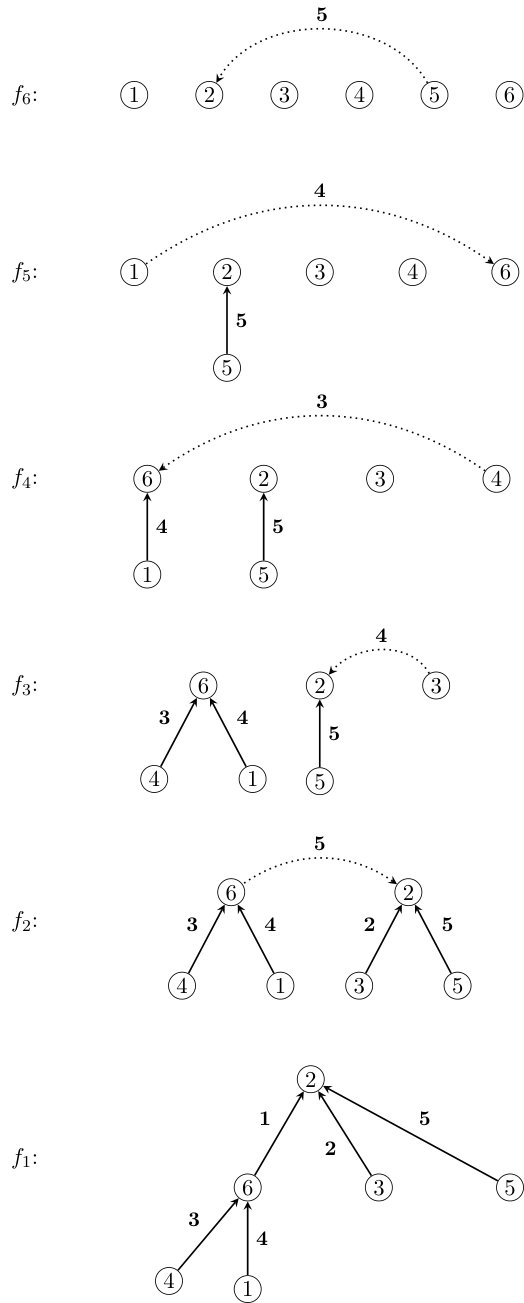 Figure 1
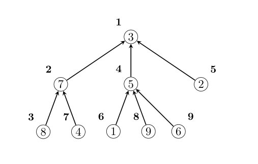 Figure 2
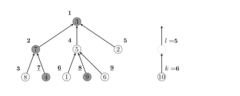 Figure 3
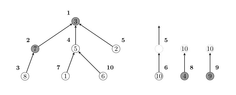 Figure 4
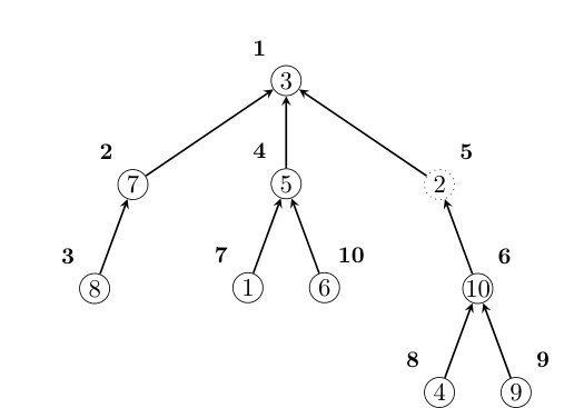 Figure 5
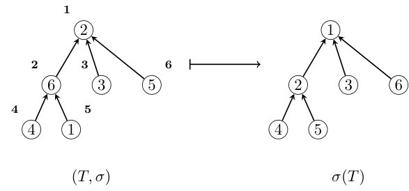 Figure 6
Peer Reviews
No public reviews on file for this paper yet. If you reviewed it on a platform where reviews are public (OpenReview, ICLR, NeurIPS, ICML), you can paste yours below so the community can read it here.
Videos
No videos yet. Explain this paper in a talk, walkthrough, or lecture? Add one.
A non-increasing tree growth process for recursive trees and applications
Laura Eslava
(Date: June 22nd 2018)
Abstract.
We introduce a non-increasing tree growth process , where is a rooted labeled tree on vertices and is a permutation of the vertex labels. The construction of from involves rewiring a random (possibly empty) subset of edges in towards the newly added vertex; as a consequence with positive probability. The key feature of the process is that the shape of has the same law as that of a random recursive tree, while the degree distribution of any given vertex is not monotonous in the process.
We present two applications. First, while couplings between Kingman’s coalescent and random recursive trees where known for any fixed , this new process provides a non-standard coupling of all finite Kingman’s coalescents. Second, we use the new process and the Chen-Stein method to extend the well-understood properties of degree distribution of random recursive trees to extremal-range cases. Namely, we obtain convergence rates on the number of vertices with degree at least , , in trees with vertices. Further avenues of research are discussed.
Key words and phrases:
Tree growth processes, Kingman’s coalescent, random recursive trees, coupling, Chen-Stein method, extreme values
2010 Mathematics Subject Classification:
60C05, 05C80.
1. Introduction
In a paper of 1970 [21], Na and Rapoport presented the problem of modeling how the structure of networks (as sociograms, communication and acquaintance networks) emerge through time. They considered two cases: * ‘growing’* trees and ‘static’ trees. The ‘growing’ model is now know as uniform attachment model and each instance is usually named (random) recursive tree. These are part of a broad class of tree growth models where vertices are sequentially added and connected to a random vertex in the current tree. On the other side, the term ‘static’ was motivated by the fact that this construction starts with the vertices the tree is aimed to have and edges are added one by one (without creating cycles). The ‘static’ model was an early description of what is now referred to as coalescent processes. The seemingly two distinct models of growth have been shown to be related for certain coalescent procedures (e.g. additive and Kingman’s); that is, their resulting trees can also be constructed by a growth process [1, 20, 22]. In particular, Kingman’s coalescents correspond, for any fixed number of vertices , to recursive trees; see Remark 2.3.
Here we present a non-increasing tree growth process where is a rooted labeled tree on vertices and is a permutation of the vertex labels. The three key features of this new growth process are:
- (1)
The shape of has the same distribution as that of recursive trees (vertices are labeled uniformly at random), 2. (2)
adding edges according to the permutation (in reverse order), recovers Kingman’s coalescent, 3. (3)
there is a positive probability that .
Formally, we introduce the class of decorated trees on vertices and a random mapping such that for all . Our main result, Theorem 1.1, states that recursively applying the mappings to the unique element in gives uniformly random decorated trees on ; from which the properties above are recovered. The fact that we can construct recursive trees in a non-increasing fashion is, to the best of our knowledge, a novel idea and it opens a wide range of further avenues of research. We discuss some of them in the last section.
We call Robin-Hood pruning to the random mapping that builds from ; it is the key conceptual contribution of this work and builds on the correspondence between recursive trees and Kingman’s coalescent exploited in [2, 10]. It seems that such connection had been rarely exploited, with exception to [6, 23], where an equivalent construction was used by to study union-find trees and then related to recursive trees.
Additionally, we provide applications to high-degree vertices of recursive trees and their maximum degree. Kingman’s coalescent had already been exploited by Addario-Berry and the author to describe near-maximum degrees in recursive trees, [2, 10]. With the new procedure, we are able to extract finer information about extreme degree values in recursive trees. The main underlying technique is the Chen-Stein method for convergence rates to Poisson distributions. Informally, this method approximates the law of a sum of indicator variables, by understanding how the law of such indicator variables changes when conditioning on one of them being equal to one. In our case, the sum counts the number of vertices with high-degree. The perspective of the Robin-Hood pruning allow us to understand how the vertex-degree distributions change when we condition on one of such vertex-degrees being large.
Before we continue to precise statements of our results, we introduce basic notation that will be used throughout the paper as well as the standard construction of recursive trees.
1.1. Notation
For , we write and for the set of permutations on . We denote natural logarithms by and logarithms with base 2 by .
Given a rooted labeled tree , write and call the size of . We write for the set of rooted trees with vertex set . By convention, we direct all edges toward the root and write for an edge with tail and head . For we write for the parent of , that is, the unique vertex with in . Finally, write for the number of edges directed toward in , and call the degree of . Note that .
We say is increasing if its vertex labels increase along root-to-leaf paths; in other words, if and for all (in particular, ). We write for the set of increasing trees of size . Using induction, it is easy to see that for all . Next, a tree growth process is a sequence of trees with for each . The process is increasing if for all ; this implies that for all .
Recursive trees on vertices, which we denote , are usually constructed as follows. Start with as a single node with label 1. For each , is obtained from by adding a new vertex and connecting it to ; the choice of is uniformly random and independent for each . It is readily seen that is a uniformly random tree in . It follows that the process is a random increasing tree growth process.
1.2. The new growth process
In what follows we extend the concept of increasing trees. If and then is the tree with edges . In words, is obtained from by relabeling the vertices of according to the permutation ; see Figure 1 for an example. We say that is an stamp history for if is increasing. If is an stamp history for then we say that the pair is a recursively decorated tree or decorated tree, and that vertex has time stamp . We denote the set of decorated trees of size by
[TABLE]
For each , the Robin-Hood pruning is a random mapping that can be applied to any decorated tree. The exact definition of will be given in Section 3. Broadly speaking, is obtained from by pruning some subtrees of and placing them as subtrees of a new vertex labeled ; additionally, vertex attaches to a random vertex or becomes the root of the new tree. The stamp history in is adjusted from such that vertex has a uniformly random time stamp. Heuristically, the random procedure follows a ‘steal from the old to give to the new’ scheme; that is, once the time stamp of has been determined, vertices with an earlier time stamp have larger probability of being reattached to vertex .
The content of our main theorem says that, when the input of is uniformly random in the output is uniformly random in . For the remainder of the paper, for any , the pair denotes a uniformly random element in . Such result boils down to carefully setting up the distribution of the random parameters involved in the Robin-Hood pruning.
Theorem 1.1**.**
For each , the Robin-Hood pruning provides a coupling between and such that .
Note that , thus the Robin-Hood pruning can be unambiguously applied to decorated trees starting from . Theorem 1.1 implies that the tree growth process given by is composed of uniformly random decorated trees, but it yields a non-increasing growth process on trees. This occurs since the rewiring may destroy some subtrees in the previous tree; see Remark 3.4. However, the shape of has the same law as that of ; this is proven by a straightforward bijection between and .
Proposition 1.2**.**
For each , and if is chosen uniformly at random then is a recursive tree of size and is a uniformly chosen permutation in .
Proof.
By definition, if , then . Let be defined such that . For an increasing tree and , let then , it is also straightforward that is injective. Therefore, . The result follows since bijections preserve the uniform measure on finite probability spaces. ∎
Growth procedures naturally couple families of trees as the size varies. For example, Proposition 1.3 below shows that is a representation of Kingman’s coalescent on ; informally, the stamp history encodes the addition of edges in the coalescent. Precise definitions are given in Section 2, for the moment it suffices to say that denotes a Kingman’s coalescent, where the are forests.
Proposition 1.3**.**
Let be uniformly random in and be a Kingman’s coalescent. Denote , then and the forests evolution is given by .
Typically there is no simple coupling of finite -coalescent processes as varies. The first application of Theorem 1.1 is that the Robin-Hood pruning produces, given a Kingman’s coalescent on vertices, a Kingman’s coalescent on vertices.
Corollary 1.4**.**
The tree growth process , coupled as in Theorem 1.1 gives an explicit coupling of all finite Kingman’s coalescents.
The proof of Proposition 1.3 is given in Section 2 and is based on previous connections between recursive trees and Kingman’s coalescents; see Remark 2.3.
1.3. High-degree vertices in
In this section we establish a phase change on the number of high-degree vertices in recursive trees. Phase changes occurs on random structures when a class of variables undergo a transition from asymptotic normal limits to asymptotic Poisson limits. The change is marked by the mean of the variables going from infinite to bounded. In recursive trees, for example, the number of fringe trees of a given size undergoes a phase change when the size of the trees tend to infinite and no longer holds [12]; similar results are given when the fringe trees are required to satisfy any given property or pattern [5, 16]. For an integer , let us count the number of high-degree vertices by
[TABLE]
and write . The following estimates where implicitly given in [2] and a proof can be found in Appendix A, Proposition 6.3. For each , there is such that uniformly over ,
[TABLE]
It thus follows that the phase change occurs when . Using a Poisson approximation together with (1) we obtain the following phase change for the counts on high-degree vertices.
Theorem 1.5**.**
For each there exists such that if , then
[TABLE]
If , under sequences for which we have that
[TABLE]
Remark 1.6**.**
Counting the high-degree vertices is equivalent to count fringe trees (of all sizes) with a high-degree root. Therefore, the asymptotic normal distribution of , (2), follows from [16, Corollary 1.25]; however, the computation of both the mean and variance for the renormalization of the variables is not seemingly straightforward. Nevertheless, we remark that the associated convergence rates in Theorem 1.7 are strong and novel.
Previous results on the profile of recursive trees consider , for . For finite values of , Janson established the joint limiting distribution of in [17]. Addario-Berry and the author addressed the case , providing all the possible limiting distributions of and establishing asymptotic normality for when and slowly tends to infinity [2].
Theorem 1.5 follows from the convergence rates of the next theorem, which in turn, applies the Chen-Stein method to . By changing the perspective of recursive trees to the distribution equivalent we can use the Robin-Hood pruning to understand how the variables change when conditioning to . The details of this approach are somewhat delicate, so we defer the discussion to Section 4.
Theorem 1.7**.**
Fix . There are constants and such that uniformly for satisfying ,
[TABLE]
Remark 1.8**.**
A detailed but simple track of the conditions on , see Proposition 4.1, shows that there is a non-empty interval such that if , then the bounds in Theorem 1.7 are, in fact, tending to zero.
Remark 1.9**.**
The exponent is determined by almost negative correlation between pairs of vertices in (see Proposition 4.1), while the exponent depends on an auxiliary coupling based on the Robin-Hood pruning (see Proposition 4.4). We believe that the constraint on could be relaxed by obtaining uniform bounds on rather than .
Finally, consider now the maximum degree of a recursive tree . Note that if and only if . Therefore, having indicates . In fact, Devroye and Lu showed that a.s. [7]. The first tail bounds on where obtained for with using singularity analysis of generating functions [13]. The relation between recursive trees and Kingman’s coalescent provided simpler proofs to such results, extending it also to [2]. The bounds in Theorem 1.7 yield broader, tighter bounds.
Corollary 1.10**.**
There exists such that uniformly over ,
[TABLE]
where .
The maximum of i.i.d. random variables is, under rather general conditions, distributed in the limit as the Gumbel (or double-exponential) distribution [15]; however lattice distributions are excluded from this regime. Addressing the case of integer-valued variables, Anderson gives sufficient conditions under which the Gumbel distribution serves as an approximation for their maximum [3]; among those is the geometric distribution. Now, when we randomize the labels in (e.g. using the tree instead), vertex degrees become exchangeable and their limiting distributions are geometric. Although, the degrees of are not independent, their correlations are weak and the Gumbel-type approximation still arises for the distribution of . Goh and Schmutz provide an alternative heuristic based on the fact that , with slowly, is asymptotically normal [13].
Outline
The paper is divided into two parts. First, we discuss more on the connection between recursive trees, Kingman’s coalescents and other tree models in Section 2. The precise definition of the Robin-Hood pruning together with the proof of Theorem 1.1 is given in Section 3. Second, the results on high-degree vertices of recursive trees use the Chen-Stein method and the Robin-Hood pruning in a non-trivial way. An overview on how we use the Chen-Stein method is given Section 4. Assuming the existence of an auxiliary coupling (Proposition 4.4), we complete the proofs concerning high-degree vertices in Section 4.1. The auxiliary coupling, based on the Robin-Hood pruning, is presented in Section 5. And finally, Section 6 discusses further avenues of research.
2. Kingman’s coalescents and recursive trees: distinct representations
Discrete coalescents are processes on partitions of that can be represented with different tree structures. On can encode the coalescent using an -chain: a sequence of forests where, at all times there are vertices (or elements), and edges are added one by one until a tree is formed. However, there is an more traditional construction using binary search trees (BST) where internal nodes correspond to merges and only external nodes correspond to elements of the coalescent. In the next section we introduce the representation used in this paper and prove Proposition 1.3. Following that, we discuss the well-know bijection between BST’s and recursive trees and the difference between the two coalescent representations. In addition, we explain the difference between the Yule-Harding model of phylogenetic trees and its uniform model, and highlight the importance of clarifying both the rules applied to the mergings in coalescent processes and their representation as trees.
2.1. Recursive trees perspective
Na and Rapoport loosely described this process as the construction of ‘static’ trees with vertices [21]:
“Initially, single elements move about at random. Each collision forms a couple. A collision of a couple with a single element forms a triple, a collision of an -tuple with a -tuple forms an -tuple, and so on. At each collision a link is established between an element of one -tuple and an element of another, the links being rigid so that the elements of the same -tuple cannot collide. The process goes on until the entire set of elements has been joined into an -tuple.”
By changing the rule on how to link the elements on the tuples, we obtain distinct coalescent distributions. In the description in [21] there are no restrictions on the elements allowed to be linked during the coalescent111Unfortunately, it was incorrectly presumed in [21] that ‘static’ trees build uniformly random unrooted labeled trees.. In fact, the discrete multiplicative coalescent arises when any possible link is chosen uniformly at random. It is associated with Kruskal’s algorithm for the minimum weighted spanning tree problem [1].
Kingman’s coalescent is characterized by the property that the merging probability of any pair of components is independent of the components’ sizes. The representation used in this paper uses that, at each time the representative of each ‘tuple’ is the current root of the tree and it is closely related to the ‘union-find’ algorithm used in computer science (see e.g. [24]). A formal description follows.
A forest is a set of trees with pairwise disjoint vertex sets. Denote by and , respectively, the union of the vertex and edge sets of the trees in . For , an -chain is a sequence of elements of such that, for , is obtained from by adding a directed edge between the roots of some pair of trees in . In particular, consists of one-vertex trees and consists of a single tree on vertices denoted by . For an example see Figure 2.
Next we introduce the necessary notation to define Kingman’s coalescent using -chains. For an -chain and , list the trees of in increasing order of their smallest-labeled vertex as . Independently for each let be uniformly chosen at random; in addition, let be independent Bernoulli random variables with mean .
Definition 2.1**.**
Kingman’s -coalescent is defined as constructed as follows. For , is obtained from by adding an edge between and . If then direct the edge towards ; otherwise direct it towards . The forest consists of the new tree and the remaining unaltered trees from .
In other words, if is a Kingman’s coalescent, then each of the trees of correspond to a set of coalesced elements after steps of the process. At each step, two sets (represented by their roots) coalesce and a new representative is chosen uniformly at random.
To link -chains with decorated trees, we first define a natural edge labeling that tracks the number of trees left in the forest when a give edge comes along. Fix , for each , let
[TABLE]
We next define a vertex labeling . Let , and for each , let
[TABLE]
The following proposition shows that the pair contains all the information to recover the original -chain ; in other words, if denotes the set of -chains, then and are in bijection.
Proposition 2.2**.**
Let be defined as follows. For an -chain , let . Then is a bijection.
Proof.
First, we show that and have the same cardinality. To count the number of -chains, consider constructing by deciding which edge to add from to . Since there are trees in , when we have chosen , there are possible directed edges to add. Therefore, .
Next, let be an -chain. For each , the new edge in joins the roots of two trees in and is directed towards the root of the resulting tree. Thus, the labels decrease along all paths in towards the root . Consequently, the labels are, indeed, an stamp history of . It follows that is well defined.
Finally, let , be distinct -chains and write . If then and clearly, . Otherwise , and the (unique) edges and are distinct. It follows that and so . This shows that is injective, and so is a bijection between and . ∎
Using the bijection of Proposition 2.2, it follows that Proposition 1.3 boils down to showing that is uniformly random in .
Proof of Proposition 1.3.
Let be a Kingman’s coalescent. For any fixed -chain ,
[TABLE]
Among the possible oriented edges connecting roots of , exactly one of them can be added to to yield . Thus, regardless of the sequence ,
[TABLE]
Recall . By Proposition 2.2, and it has a uniform distribution, since the bijection preserves the uniform measure of . Finally, by Proposition 2.2, it follows that . The evolution of the forests is given by ; equivalently by . ∎
Remark 2.3**.**
It follows from Propositions 1.2 and 1.3 that, for any fixed and up to relabeling of vertices, Kingman’s coalescent correspond to recursive trees. See also [1, 2] for direct proofs of this fact.
2.2. The binary search tree connection
Binary search trees have been related to both recursive trees and phylogenetic trees. In this section we briefly discuss these connections and compare them with Kingman’s coalescent. Let be the set containing all plane, rooted, unlabeled binary trees with external nodes. Trees in distinguish between left and right subtrees of any given internal vertex. It can be shown that the sizes are given by the Catalan numbers.
Binary search trees are the tree representation of the sorting algorithm Quicksort. Simply described, for each , the quicksort algorithm takes a permutation and constructs (step by step) a binary tree with internal vertex labels on as follows. The root is and vertices are sequentially added so that the final tree satisfies the following property: for any internal node , all nodes on its left subtree are smaller than and all nodes on its right tree are larger than . It follows that, given a shape of a binary tree , there is exactly one way to label internal vertices.
There are distinct permutations as input for the quicksort algorithm. Devroye introduced the representation of the binary search tree (process) using time stamps which record all the insertion process. Using this representation, the rotation correspondence maps (one-to-one) recursive trees (on vertices) and binary search trees (with external vertices). For a thorough description of the correspondence see [16, Section 2, Figures 1-2].
On the other side, phylogenetic trees on species are represented by elements in . In this case, species are assumed to have a common ancestor (the root), internal nodes are also ancestors and the time elapsed between differentiation of species, length of the branches, is omitted. Two common distributions on phylogenetic trees are the uniform one, known as the Catalan model, and the Yule-Harding model. The latter is a process that constructs trees starting from the root, by branching a uniformly random external node and replacing it with a cherry (an internal node with two external nodes). Clearly, this construction corresponds one-to-one to the quicksort algorithm. We remark that the Yule-Harding process does not yield uniform phylogenetic trees (as neither the BST is uniform in ). For further discussion between the two models, see e.g. [4, Section 3].
It has been presumed that Kingman’s coalescent is the bottom’s up construction of the Yule-Harding model, see e.g. [5]; however, such correspondence has to be done carefully, as merges in principle are not bound to satisfy planarity constraints. As we can see through the bijections and -to-1 mappings from Propositions 2.2 and 1.2, there should be a correspondence between BST’s with time stamps and Kingman’s coalescent.
The construction of Kingman’s coalescent as a binary tree in with time stamps is the following. Using the same random variables used in Definition 2.1, add an internal node connecting the two roots of the merging trees, while the coin flip indicates which of the trees is left child of the new internal vertex; the time stamps indicate the (reversed) order of addition of internal nodes. Note that in this construction, the symmetry breaking of the coin flip is still necessary.
Conversely, we describe how to interpret time stamps of a BST as the merging history of a Kingman’s coalescent. To do so, we have to label external nodes uniformly at random (so that there are a total of different processes). Now, the role of internal vertices is as follows. At step , the two set of external vertices in each of the subtrees of the vertex with time stamp are the subsets to be merged in the coalescent.
Kingman’s coalescent has uniform distribution when considering all possible merging histories with elements labeled exchangeably. However, considering only the final tree (either in or ) yields a non-uniform distribution: there are total ways to merge the subtrees (if we use the symmetry breaking at each merging), but there are only and different rooted, labeled trees and phylogenetic trees, respectively.
3. The Robin-Hood pruning
The Robin-Hood pruning is a random procedure based on randomizing the parameters of a deterministic mapping where the set defines all possible ways to prune a decorated tree on vertices. The distribution on is tailored so that the Robin-Hood pruning, in fact, yields a coupling of .
First we introduce the necessary notation to define , the deterministic pruning and verify that, indeed, the mapping is well defined. We then continue to define the distribution on used in defining the Robin-Hood pruning (Definition 3.5). The proof of Theorem 1.1 requires us to characterize the properties of the uniform distribution in decorated trees. For the characterization in Lemma 3.6 and the proof of Theorem 1.1, we underline the difference between deterministic elements of and random elements using bold notation; the distribution of is not given a priori.
3.1. A deterministic process
Informally, we define all possible ways to prune a decorated tree on vertices using three parameters : the time stamp of the new vertex, its point of attachment given by time stamp, and the vertices to be rewired encoded by time stamp in the sequence . Once a stamp history is given to a tree , contains the vertices to be pruned and rewired towards the new vertex .
We now proceed to precise definitions. Let and set
[TABLE]
additionally, for and a permutation , let
[TABLE]
Remark 3.1**.**
The definition of is such that if and only if .
The following deterministic pruning is illustrated in Figure 3.
Definition 3.2**.**
Fix , and . We define and set
[TABLE]
as follows. First, let and construct from : For each , replace the edge with an edge connecting to a new vertex labeled . Now, if then attach to ; otherwise, attach vertex to . In other words, the edges of are given by
[TABLE]
Second, let be defined by and for ,
[TABLE]
Lemma 3.3**.**
For any , is well defined. That is, for any and ,
[TABLE]
Proof.
Write . When , it is clear that is a tree. When , let be the parent of in and let be the path from to the root of . Since is a stamp history of , ; moreover, . It follows that for all and consequently, no edges in the path from to the root in closes a cycle by connecting to .
Now, we show that is a stamp history for . It is clear that is a permutation of , so it suffices to prove that , for all . First, for vertices with we have and consequently .
Second, consider with . It follows that and thus . Consequently, and so . The last case occurs when and . We then have . ∎
Remark 3.4**.**
Whenever has for some , setting and yields . This implies that .
3.2. The random process
The -set is a sample of according to the following distribution.
Definition 3.5**.**
Fix . Let ; if let , and if let . Independently, let where are independent variables. An -set is a triple of random variables with the same law as .
We are ready to define the Robin-Hood pruning. For each , let be an -set and define
[TABLE]
The law of depends on the initial input ; however, the distribution of the -set is tailored so that preserves the uniform measure on decorated trees. In order to prove Theorem 1.1, we start with a characterization of .
Lemma 3.6**.**
Let be an integer. A random decorated tree is uniformly random if and only if the following properties are satisfied.
- i)
The permutation is uniformly random on . 2. ii)
Conditionally given , the vertices are independent. 3. iii)
For all vertices and indices ,
[TABLE]
Proof.
Let be uniformly random on . Condition follows directly from Proposition 1.2 which states that is a uniformly random permutation and has the law of a recursive tree . In addition, Proposition 1.2 implies
[TABLE]
from which conditions and immediately follow: Parents in recursive trees are chosen independently for each of the vertices, and for all ,
[TABLE]
Now consider a random decorated tree satisfying conditions -. Fix a decorated tree , and for , let . Condition on the conditional independence of parents gives, for ,
[TABLE]
Using that is an stamp history for , so , and that is uniformly random, it follows from (3) that
[TABLE]
Any increasing tree is determined by the set of parents . Using that and the conditional independence from condition we get
[TABLE]
the last equality holds by (4) and the fact that . Finally, using the equation above and that is uniformly random, we have
[TABLE]
This holds regardless of the choice of , so is uniformly random in .
∎
We are now ready to prove Theorem 1.1.
Proof of Theorem 1.1.
Let be a uniformly random decorated tree. Let be an -set and let . It suffices to show that satisfies the properties in Lemma 3.6.
First, condition follows from the construction of and the distributions of both and . Second, once conditioning on , which is equivalent to conditioning on both and , we get
[TABLE]
where the last two sets are conditionally independent given . Now, since is uniformly random in , the parents are independent, conditionally given (and thus, also conditionally given ). On the other hand, for with ,
[TABLE]
Note that is determined independently from other vertices, thus are also independent, conditionally given . This implies that condition is satisfied.
Third, fix and fix distinct . We consider three cases; namely , , and . Let
[TABLE]
It remains to show that the probabilities of are given by (3) for all . The event implies that . Therefore, occurs precisely when , , and . Then,
[TABLE]
Next, implies that and thus . It then follows that occurs when , , and . Therefore,
[TABLE]
For the last case, since , it follows that . For each let
[TABLE]
In computing the probabilities we use that is uniformly random in . If , then both and ; in addition, only if . Therefore, if , then
[TABLE]
Similarly, if , then , , and additionally . It then follows that, if ,
[TABLE]
We have shown that is uniform for all , and we get
[TABLE]
Altogether, we have shown that condition is satisfied and so the proof is complete. ∎
4. The Poisson approximation
Recall that is a uniform decorated tree and that has the shape of a recursive tree. In fact, Proposition 1.2 implies that the following distributional identity holds, for all ,
[TABLE]
It follows that the distribution of and does not change if we redefine them as and . However, the correlations in have a subtle difference in comparison with those in . To see this, observe that is negative orthant dependent; for a definition see [8]. This fact can be proven by induction from the two-vertex case , which, in turn, follows essentially from the negative orthant dependency of multinomial distributions, see e.g. [7, Lemma 1]. As a consequence, for all ,
[TABLE]
On the other hand, the following proposition gives conditions on for the degrees in to have a pairwise ‘almost’ negative correlation.
Proposition 4.1**.**
For any there exists such that uniformly for and distinct ,
[TABLE]
Moreover, .
We make precise the constraints on as this is crucial to Theorem 1.5. A weaker version of Proposition 4.1, without explicit error bounds, was proved in [2, Proposition 4.2]; a complete proof of Proposition 4.1 appears in Appendix A.
Although we do not claim the bounds in Proposition 4.1 are optimal, it seems that the property in (5) is lost when randomizing the vertex labels of to obtain . The bound in (6) will be an important input to the Chen-Stein Method.
Briefly explained, our application of the Chen-Stein method compares, in total variation distance, the sum with respect to a Poisson variable with mean . The strength of the bounds depend on finding suitable couplings between and conditional versions of such variables. More precisely, we use the pruning procedure to obtain and Fact 5.1 describes in terms of the independent elements and . This allows us to analyze the conditional law of given holds.
Before going into further details we layout the necessary notation. Given probability measures and , a coupling of and is a pair of random variables (either real or vector-valued) with and . Let be a collection of -valued random variables. Let be the law of and for let be the conditional law of given that , so
[TABLE]
We use the Chen-Stein method stated below.
Theorem 4.2** ([14, Theorem 3.7]).**
Let be a collection of -valued random variables and let . For each fix a coupling of and . Then with , we have
[TABLE]
To apply Theorem 4.2 with as tight as possible bounds, one can exploit properties of the variables or construct couplings of and with specific properties.
Corollary 4.3**.**
Let be a collection of -valued random variables and let . If the variables are exchangeable, then for any fixed and coupling of and , we have
[TABLE]
If, moreover, and there is a coupling of and satisfying for all , then
[TABLE]
Now, for the remainder of the section, fix and let, for all , , so that . Let be a coupling of and where is the law of and is the conditional law of given that .
If we would have orthant negative correlation for then it would follow that for all , and so the conditions for (8) would be satisfied. Although such strong property has not been yet established, Proposition 4.1 implies for each ,
[TABLE]
This suggests that there are couplings of and for which, with high probability, for all . The existence for such couplings is delicate as the inequality has to hold for all simultaneously.
The next proposition is the key ingredient in applying the Chen-Stein method to prove Theorem 1.7. The coupling is based on the Robin-Hood pruning and its proof is the content of Section 5.
Proposition 4.4**.**
Let . There is such that for any there exists a coupling of and , in which for all ,
[TABLE]
In the next section we assume Proposition 4.4 and complete the proofs of the results on high-degree vertices of .
4.1. Proofs for high-degree vertices
Proof of Theorem 1.7.
Fix and let . We apply the Chen-Stein method to . First, we use the coupling of and given in Proposition 4.4. By (7), we have
[TABLE]
It thus remains to show that the terms in the bound above are , where and are defined as in Propositions 4.1 and 4.4 respectively. For any ,
[TABLE]
The terms in the last line are bounded by (6) and Proposition 4.4, respectively. Since (1) gives we get
[TABLE]
Finally, (1) together with also gives . ∎
Proof of Theorem 1.5.
Fix and let be as in Theorem 1.7. Using the upper bound for in Proposition 4.1 and simple computations yield . Thus, we can chose . Let be such that . By the choice of and , we have that, as , ; while (1) implies
[TABLE]
The result then follows by Theorem 1.7 and the central limit theorem of Poisson variables, see e.g. [9, Exercise 3.4.4].
∎
Proof of Theorem 1.10.
Recall that . Let satisfy , where is a constant to be determined below, and note that . Let and .
We have that if and only if . Therefore,
[TABLE]
We deal with the two terms on the right-hand side of (9) separately. First, using the lower bound on , there is a constant such that for large enough, . Therefore, (1) gives such that . Consequently,
[TABLE]
For the second term in (9), Theorem 1.7 gives such that
[TABLE]
It remains to deal with these two error terms. Note that . Therefore, if then
[TABLE]
similarly, for large enough,
[TABLE]
The two limits above imply that , completing the proof.
∎
5. The coupling for the Chen-Stein Method
In this section we define and analyze the auxiliary coupling used in Proposition 4.4. The coupling is based on the following straightforward property of the deterministic pruning.
Fact 5.1**.**
Fix . For , we have , and for ,
[TABLE]
In words, Fact 5.1 specifies when the degree of a vertex changes: either for having as a new child or for losing children that are rewired towards . Clearly, the degree of equals the total number of such rewirings.
The heuristic for the almost negative relation obtained in Proposition 4.4 is the following. Start with and apply the Robin-Hood procedure. If the degree of vertex is large, Fact 5.1 implies that a large number of vertices in were rewired towards in the new tree; thus, many (parent) vertices decreased their degree by at least one. In short, conditioning on implies that other vertices are (slightly) less likely to satisfy .
For the remainder of the section, fix , and . Let be uniformly random in , be an -set, and be distributed as an -set conditioned to satisfy . Now, write
[TABLE]
To avoid cluttery notation, we omit the dependency on of the conditional random variables and . By Fact 5.1 and Theorem 1.1, is a conditional version of given that . Consequently, if and for all , then any coupling between and yields a coupling for the measures and in Proposition 4.4.
Our goal is then to couple and in such a way that the negative relation between and fails on a negligible set. More precisely, we construct a coupling so that there is satisfying
[TABLE]
Lemmas 5.2–5.4 provide the coupling between and , while Proposition 5.5 gives necessary conditions, under the coupling, for to hold. The proof of Proposition 4.4 then follows from bounding the probability that such necessary conditions occur.
5.1. Construction of the coupling
For any integer , let be a conditional version of given that . The following observation is quite standard but we include a proof for completeness. For and , only if for all . We say that is monotone if and imply .
Lemma 5.2**.**
For each , there exists a coupling of and such that for all .
Proof.
Fix . Note that is a monotone subset of . Harris inequality implies , for any monotone subset . Dividing through by yields . Therefore, stochastically dominates . The existence of the coupling is then guaranteed by Strassen’s theorem [19]. ∎
Before the next coupling, we gather two observations. First, for fixed , we have . To see this, observe that can be rewritten as
[TABLE]
the claim then follows by the independence between and . Second, the sequence is proportional to and, thus, it is decreasing in . Clearly, the latter sequence of probabilities is decreasing in , while both are proportional with a factor . To see this, use the independence between and to obtain
[TABLE]
Lemma 5.3**.**
There exists a coupling of and such that and .
Proof.
Let be independent with and independently, let be i.i.d. . By a slight abuse of notation we redefine the variables and using the variables and argue that the original law is preserved.
Let and with
[TABLE]
It is straightforward that and have the correct law by construction, while has the correct law since for each . Moreover, since is decreasing, it follows that implies . It follows that , and so . ∎
Lemma 5.4**.**
There exists a coupling of and such that , and for all .
Proof.
Let be i.i.d. and independently, let be independent with . For each fix a vector coupled with according to Lemma 5.2. The dependence structure of is unimportant to the argument, but for concreteness we may, e.g., take them to be conditionally independent given . On the other hand, it is important to insist that the are independent of . Since we will define using , the existence of such joint coupling is straightforward.
Again, by a slight abuse of notation we redefine the variables and argue that the original law is preserved. Define , as in Lemma 5.3 and let . Clearly, is an -set. It remains to show that has the conditional distribution of given that . For any , the probability can be rewritten as
[TABLE]
Adding two factors of and using the independence between and , we can factorize these probabilities as
[TABLE]
These probabilities correspond, respectively, to the distributions of and , which are independent. Therefore,
[TABLE]
as desired. Finally, the variables and satisfy the desired inequalities by Lemmas 5.2 and 5.3. ∎
5.2. Analysis of the coupling
The proof of Proposition 4.4 boils down to understanding necessary conditions for to hold under the coupling of Lemma 5.4.
Proposition 5.5**.**
Consider and defined in Lemma 5.4 and their corresponding decorated trees defined in (10) and (11). For any ,
[TABLE]
Proof.
From the properties of the coupling in Lemma 5.4,
[TABLE]
Consequently, using Fact 5.1 we have that . On the other hand, if holds, then it follows that and so it is necessary that holds. Finally, implies that
[TABLE]
or equivalently, that . ∎
We can also argue, more specifically, that
[TABLE]
however, the approach we chose allow us to use uniform bounds for all . We will frame the events from the perspective of recursive trees where the degree distributions are distinct for each vertex. Recall the following version of Bernstein inequalities (see, e.g. [18] Theorem 2.8, (2.5)). For a sum of -valued variables and , . By the construction of we have that where are independent Bernoulli variables with mean . Therefore,
[TABLE]
Using that , we can apply Berstein’s inequality with and set . It follows that there is such that uniformly over , and ,
[TABLE]
Proof of Proposition 4.4.
Fix . Let and be as in (14). Let and be as defined in (10) and (11) with as in Lemma 5.4. Set and for all , so that is a coupling of the measures and .
Our goal is to bound . First, by Proposition 5.5,
[TABLE]
Next we obtain uniform bounds for the terms on the right-hand side. Recall that is a uniformly random permutation independent of and that . These facts, together with (14) gives, for each ,
[TABLE]
Plugging together these bounds, we get for any ,
[TABLE]
∎
6. Conclusions and further research
The Robin-Hood pruning yields an interesting process . By Theorem 1.1 and Proposition 1.2, for all ; that is, has the shape of a recursive tree. The novelty of this process is that the Robin-Hood pruning is a fairly complex dynamic of trees which has potential connections to mathematical models of social and economic networks and raises challenging theoretical questions.
First, only asymptotically about half the time is obtained from by simply attaching to a uniformly random vertex. To see this, recall that where (see Fact 6.1 and Lemma 6.2). It follows that with probability tending to the newly added vertex will be a leaf. Second, for all , a.s. , while Fact 5.1 and the distribution of the -set yield
[TABLE]
Third, from time to time, a large proportion of edges will be rewired towards the newly added vertex, drastically reshaping the structure of the tree. For example, for any ,
[TABLE]
As for applications, in the context of random networks, the Robin-Hood pruning has an interpretation in terms of ‘trends’; for example, a new vertex brings in a new idea to the network which may drastically rewire the interests or connections of established individuals in the network. The stamp history gives a ranking between the elements of that determines the susceptibility of changing parents in the tree. Preferential attachment models are considered better models for real-world networks. It would be interesting to devise a similar pruning procedure that, acting on preferential attachment trees, preserves their scale-free degree distribution.
In the context of biology, Kingman’s coalescent is usually represented with increasing binary trees, keeping individuals as external nodes and adding an internal node for each merge between two lineages. The representation using -chains breaks the symmetry between the pairs of trees merging at each step. Thus, it is not clear how the Robin-Hood pruning process would have a significant interpretation in terms of the genealogical information.
Regardless of the perspective we use to motivate the process , there are many interesting theoretical questions that would be worth pursuing. To name just a few:
- (1)
Understand the process describing how the parent and descendants of a given vertex change with time.
- •
Describe how the size of the subtree rooted at a fixed node evolves.
- •
How does maximum size of such subtree grow? 2. (2)
Understand the maximum degree dynamics in both and .
- •
How often does vertices attaining the maximum degree change?
- •
Are this dynamics the same for both processes? 3. (3)
Determine whether there is a coupling for which the sequence is negative related (i.e. that conditions for (8) are satisfied), or similarly, whether the sequence is negative orthant dependent.
Acknowledgements
I would like to thank Louigi Addario-Berry and Henning Sulzbach for some very helpful discussions, and to the anonymous referees who provided insight on how to improve the presentation of the results and additional references. This research was supported by FQRNT through PBEEE scholarship with number 169888.
Appendix A: Proof of Proposition 4.1
We use the representation of Kingman’s coalescent that consists of a chain and write for the unique tree contained in . By Proposition 1.3 we can work with the tree . The proof mimics that of [2, Proposition 4.2], but requires a little more care as we wish to obtain explicit error bounds.
For each let denote the tree in that contains vertex . For each , the selection set of is defined as
[TABLE]
this set keeps record of the times when the tree containing merges. Finally, for each , we say that is favorable for vertices in (resp. vertices in ) if (resp. ).
The key property of Kingman’s coalescent is the following. For each , if favors , then increases its degree by one in the process; otherwise attaches to the root of the other merging tree and the degree of remains unchanged for the rest of the process. Since all vertices start the process as roots, is equal to the length of the first streak of favorable times for . Moreover, are independent and distributed as . Therefore we have the following distributional equivalence.
Fact 6.1**.**
Let be a random variable with distribution independent of , then
[TABLE]
This fact, together with the next lemma, allow us to get estimates for the tails of .
Lemma 6.2**.**
If and . Writing , we have
[TABLE]
Proof.
First, there are distinct pair of trees in , exactly of such pairs contains ; thus . Since the merging trees are chosen independently at each time, we have that for any we have
[TABLE]
where the variables are independent Bernoulli variables with , respectively. The desired bound is then a straightforward application of Bernstein’s inequalities (see, e.g. [18], Theorem 2.8 and (2.6)). For a sum of -valued variables, we have . In this case, and
[TABLE]
The result follows by setting . ∎
Proposition 6.3**.**
If and , then for ,
[TABLE]
Proof of Proposition 6.3.
It follows from Lemma 6.1 that
[TABLE]
The upper bound on is then trivial, while the lower bound follows by Lemma 6.2 using and that . ∎
Now, consider two distinct vertices . For , let contain all pairs of selection sets that enable vertices and to have degree at least ; that is, only if
[TABLE]
Since the are independent of the selection times, we have that
[TABLE]
To estimate we need more details on the dynamics of the model. We start with a simple tail bound for the following random variable; let
[TABLE]
Lemma 6.4**.**
For , .
Proof.
Vertices in are exchangeable, so we can take ; these vertices belong to distinct trees in for all . Additionally, by the ordering convention of trees in , it follows that and for all .
We claim that for all ,
[TABLE]
This follows by induction on . Clearly, only if which occurs with probability , thus satisfies the equation above. For , we have
[TABLE]
Next, for larger enough,
[TABLE]
The second inequality uses that for sufficiently small, followed by the fact that . The result follows with . ∎
Lemma 6.5**.**
If and , then for any ,
[TABLE]
Proof.
For each write , then
[TABLE]
Before, establishing (16), we note that the terms in the right-hand side of (16) are bounded by Lemmas 6.4 and 6.2, respectively. Since such bounds depend on the choice of , we can use
[TABLE]
The last equality since the functions to be minimized are decreasing and increasing, respectively, on the interval. It then follows that the maximum is attained when satisfies .
We now proceed to establish equation (16). At step , exactly one of and is favored by . Thus, at least one of or gets its degree fixed for the remainder of the process. Therefore,
[TABLE]
By intersecting with the event , and the exchangeability of vertices in we get,
[TABLE]
from which (16) follows. ∎
Proof of Proposition 4.1.
Fix , and let be defined as in Proposition 4.1. By Proposition 1.3, if follows that and
[TABLE]
the last equality by (15). Lemmas 6.5 and 6.3 then gives that for ,
[TABLE]
∎
The reference list from the paper itself. Each links out to its DOI / PubMed record.
- 1[1] L. Addario-Berry. Partition functions of discrete coalescents: from Cayley’s formula to frieze’s ξ ( 3 ) 𝜉 3 \xi(3) limit theorem. In XI Symposium on Probability and Stochastic Processes. Progress in Probability , volume 68. Birkhauser, Basel.
- 2[2] Louigi Addario-Berry and Laura Eslava. High degree of random recursive trees. Random Structures Algorithms , 52:560–575, 2018.
- 3[3] C. W. Anderson. Extreme value theory for a class of discrete distributions with applications to some stochastic processes. J. Appl. Probability , 7:99–113, 1970.
- 4[4] Blum M., Franois O and Janson, S. The mean, the variance and limiting distributions of two statistics sensitive to phylogenetic tree balance. Ann. Appl. Probability , 16:2195–2114, 2006.
- 5[5] Huilan Chang and Michael Fuchs. Limit theorems for patterns in phylogenetic trees. J. Math. Biol. , 60(4):481–512, 2010.
- 6[6] L. Devroye. Branching processes in the analysis of the heights of trees. Acta Inform. , 24(3):277–298, 1987.
- 7[7] Luc Devroye and Jiang Lu. The strong convergence of maximal degrees in uniform random recursive trees and dags. Random Structures Algorithms , 7(1):1–14, 1995.
- 8[8] Devdatt Dubhashi and Desh Ranjan. Balls and bins: a study in negative dependence. Random Structures Algorithms , 13(2):99–124, 1998.