Feynman-Kac equation for anomalous processes with space- and time-dependent forces
Andrea Cairoli, Adrian Baule

TL;DR
This paper derives a generalized Feynman-Kac equation for anomalous diffusive processes influenced by space- and time-dependent forces, extending the mathematical framework to better model complex biological and physical systems.
Contribution
It provides the first derivation of the Feynman-Kac equation for anomalous processes with space- and time-dependent forces using subordination, and extends it to functionals relevant for stochastic thermodynamics.
Findings
Derived the Feynman-Kac equation for complex anomalous processes
Extended the equation to include time-dependent functionals
Obtained exact results on work fluctuations in a non-equilibrium model
Abstract
Functionals of a stochastic process Y(t) model many physical time-extensive observables, e.g. particle positions, local and occupation times or accumulated mechanical work. When Y(t) is a normal diffusive process, their statistics are obtained as the solution of the Feynman-Kac equation. This equation provides the crucial link between the expected values of diffusion processes and the solutions of deterministic second-order partial differential equations. When Y(t) is an anomalous diffusive process, generalizations of the Feynman-Kac equation that incorporate power-law or more general waiting time distributions of the underlying random walk have recently been derived. A general representation of such waiting times is provided in terms of a L\'evy process whose Laplace exponent is related to the memory kernel appearing in the generalized Feynman-Kac equation. The corresponding anomalous…
Click any figure to enlarge with its caption.
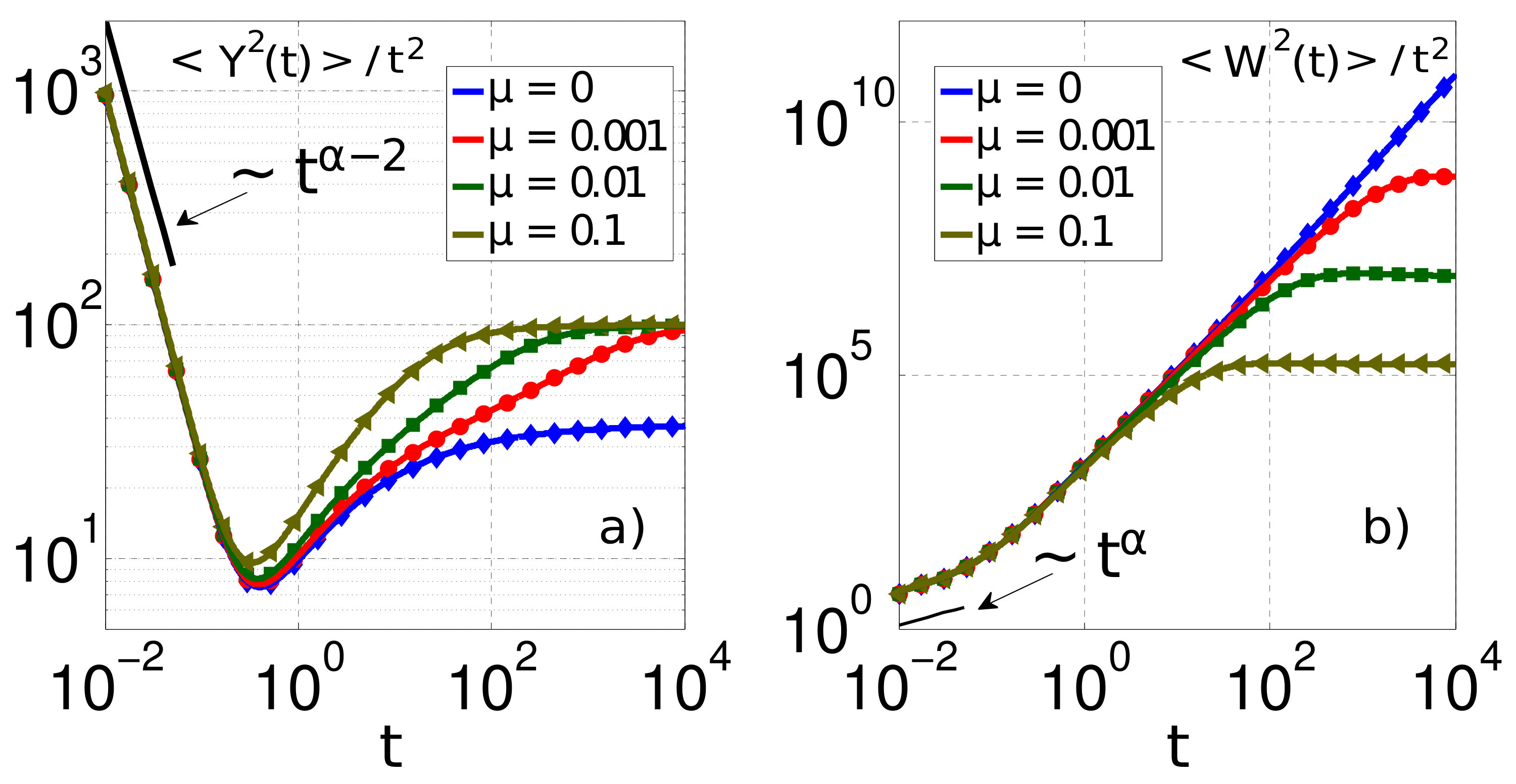 Figure 1
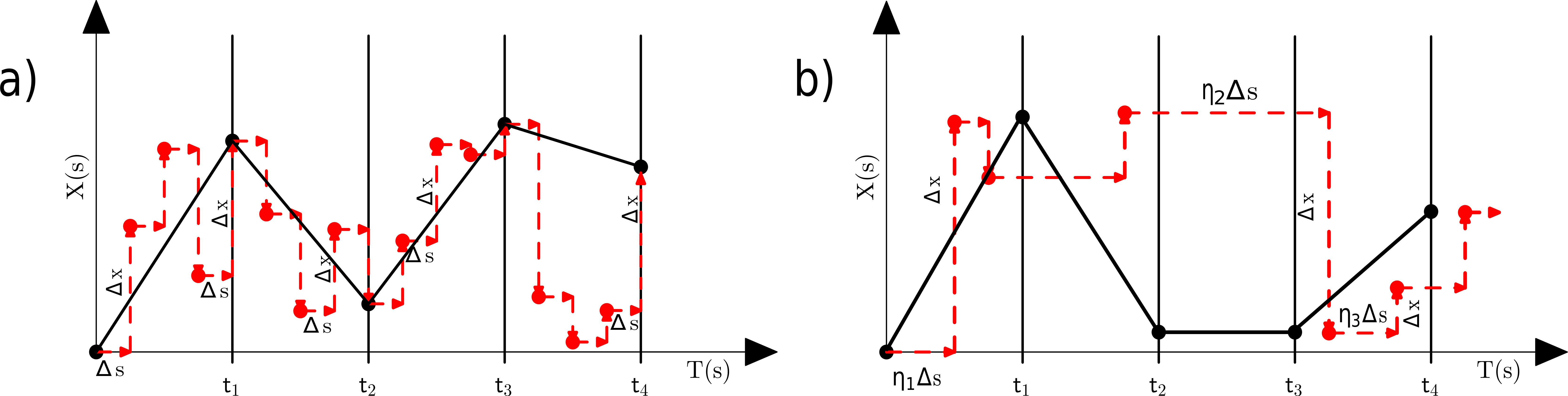 Figure 2
Peer Reviews
No public reviews on file for this paper yet. If you reviewed it on a platform where reviews are public (OpenReview, ICLR, NeurIPS, ICML), you can paste yours below so the community can read it here.
Videos
No videos yet. Explain this paper in a talk, walkthrough, or lecture? Add one.
Present address: ]Department of Bioengineering, Imperial College London, South Kensington Campus, SW7 2AZ, UK
Feynman-Kac equation for anomalous processes with space- and time-dependent forces
Andrea Cairoli
[
Adrian Baule
Corresponding author: [email protected]
School of Mathematical Sciences, Queen Mary, University of London, Mile End Road, E1 4NS, UK
(March 18, 2024)
Abstract
Functionals of a stochastic process model many physical time-extensive observables, for instance particle positions, local and occupation times or accumulated mechanical work. When is a normal diffusive process, their statistics are obtained as the solution of the celebrated Feynman-Kac equation. This equation provides the crucial link between the expected values of diffusion processes and the solutions of deterministic second-order partial differential equations. When is non-Brownian, e.g., an anomalous diffusive process, generalizations of the Feynman-Kac equation that incorporate power-law or more general waiting time distributions of the underlying random walk have recently been derived. A general representation of such waiting times is provided in terms of a Lévy process whose Laplace exponent is directly related to the memory kernel appearing in the generalized Feynman-Kac equation. The corresponding anomalous processes have been shown to capture nonlinear mean square displacements exhibiting crossovers between different scaling regimes, which have been observed in numerous experiments on biological systems like migrating cells or diffusing macromolecules in intracellular environments. However, the case where both space- and time-dependent forces drive the dynamics of the generalized anomalous process has not been solved yet. Here, we present the missing derivation of the Feynman-Kac equation in such general case by using the subordination technique. Furthermore, we discuss its extension to functionals explicitly depending on time, which are of particular relevance for the stochastic thermodynamics of anomalous diffusive systems. Exact results on the work fluctuations of a simple non-equilibrium model are obtained. An additional aim of this paper is to provide a pedagogical introduction to Lévy processes, semimartingales and their associated stochastic calculus, which underlie the mathematical formulation of anomalous diffusion as a subordinated process.
I Introduction
In experimental applications one typically measures physical observables , whose time evolution is determined by the underlying dynamics of the system, which is described by some stochastic process . Such time-extensive quantities are naturally defined as functionals of the process in the form:
[TABLE]
where is some prescribed arbitrary function. If is a normal diffusive process, these functionals have been employed to model many different physical phenomena by choosing the function suitably either with an explicit time dependence or without it. For instance, in the linear case , with interpreted as a particle’s velocity, represents its position and the – representation simply describes the stochastic evolution of the system in the phase space risken1989fokker . If instead we choose and , stands for the local and occupation time respectively darling1957occupation ; agmon1984residence ; newman1998diffusive ; berezhkovskii1998residence ; dhar1999residence ; godreche2001statistics ; majumdar2002local ; blanco2003invariance ; mazzolo2004properties ; barkai2006residence ; grebenkov2007residence ; dumonteil2016residence . Other relevant choices are with Eq. (1) interpreted as a one-dimensional spatial integral, in which case is interpreted as the variance of a fluctuating interface majumdar2005brownian , and with a real positive parameter, which describes the dynamics of integrated stock prices of the Black-Scholes type yor2012exponential . Another important class of functionals has been introduced in the context of the stochastic thermodynamics of driven small scale systems. Specifically, one is interested in the statistical properties of the accumulated mechanical work done by the system when a non-equilibrium driving is imposed by a time-dependence in a potential via some prescribed time-dependent protocol . In such a scenario, assuming to be the position coordinate, the mechanical work is defined by Eq. (1) with jarzynski1997nonequilibrium ; sekimoto1997kinetic ; sekimoto1998langevin ; sekimoto2010stochastic ; seifert2012stochastic .
In order to obtain the probability density function (PDF) of one usually considers quantities of the form:
[TABLE]
for a given initial condition . We note that is the Fourier-transform of the joint PDF of the processes and , such that, if one could compute it, the marginal PDF of would be obtained straightforwardly by making its Fourier inverse transform and subsequently integrating it over all . Equivalently to the direct evaluation of the expected value in Eq. (2), can be obtained by solving the Feynman-Kac (FK) equation majumdar2005brownian :
[TABLE]
where we introduce the most general Fokker-Planck operator for a space-time dependent force and diffusion coefficient: . In the linear case , Eq. (3) maps directly onto the Klein-Kramers equation for the joint position-velocity PDF of a Brownian particle risken1989fokker . The relevance of the FK Equation (3) is motivated by the fact that it allows the calculation of expected values over stochastic trajectories of the type of Eq. (2) in terms of solutions of second-order partial differential equations, i.e., of non-random equations, and vice versa. In the conventional setting, i.e., that of Eq. (3), the dynamics of is described by the Langevin equation:
[TABLE]
where is a Gaussian white noise with zero mean and covariance and the Itô-convention is assumed for the multiplicative term (Appendix A). Note that the FK equation contains as a special case the Fokker-Planck equation to which it reduces by setting in Eqs. (2, 3). Thus, Eq. (3) is the key method to derive the full statistics of a wide range of phenomena modeled by the diffusive dynamics of Eq. (4) risken1989fokker .
In recent years, an intense effort has been dedicated to derive generalizations of both the FK and Klein-Kramers equation, that extend beyond the normal diffusive regime into the anomalous one. First results were obtained either by substituting with a Lévy noise, such that describes Lévy flight type dynamics, peseckis1987statistical ; fogedby1994levy ; jespersen1999levy ; lutz2001fractional ; eliazar2003levy or by directly introducing temporal memory integral terms manifest in time fractional operators into the ordinary FK and Klein-Kramers equations, thus accounting for the non-Markovian effects often characterizing anomalous diffusive processes on a purely phenomenological level metzler2000generalized1 ; metzler2000subdiffusive ; metzler2000generalized2 ; barkai2000fractional ; metzler2002superdiffusive ; zoia2012discrete ; fa2013generalized . These fractional FK equations have been successfully used to model, e.g., the dynamics of migrating epithelial cells dieterich2008anomalous and the advection of a fluid particle in turbulence baule2006investigation . However, the relation between such equations and the underlying stochastic dynamics is often not clear eule2007langevin ; eule2012langevin . Thus, more systematic approaches have been adopted, which explicitly assume the process to represent a continuous time random walk (CTRW) with jump lengths and waiting times drawn from independent distributions montroll1965random ; metzler2000random . Specifically, in Friedrich2006Anomalous ; Friedrich2006Exact , starting from a random walk description of the CTRW in phase space, a Klein-Kramers equation containing a fractional substantial derivative, which generalizes the ordinary material derivative through the inclusion of explicit retardation effects, was derived. In turgeman2009fractional a fractional FK equation with the same fractional derivative was derived within a similar random walk description of CTRWs with power-law distributed waiting times. Extensions of this approach to space- and space-time-dependent forces have also been discussed in carmi2010distributions ; carmi2011fractional , as well as to inhomogeneous media in shkilev2012equations ; shkilev2016feynman .
Even if these equations are systematic extensions of the conventional FK formula, they do not establish the same correspondence between some anomalous stochastic dynamics and the solutions of fractional partial differential equations as in the conventional picture of Eqs. (3, 4). Instead of using a Langevin-type equation to describe the dynamics of the underlying CTRW, the time evolution of is derived directly by means of a generalized master equation. Such full correspondence has been established only recently in our work cairoli2015anomalous by using a general representation of the CTRW in terms of a random time change (also called subordination) of a normal diffusive process. This approach allows in particular to capture straightforwardly different waiting time distributions of the CTRW by a monotonically increasing Lévy process in an auxiliary time variable. The characteristic Laplace exponent of the Lévy process is naturally related to the memory kernel appearing in the generalized FK equation. Our FK formula has been recently confirmed in wu2016tempered , within a random walk approach, for the special case of tempered Lévy-stable distributed waiting times.
As shown in cairoli2015anomalous , by employing a variable parametric form of , one can fit the resulting anomalous process to mean-square displacement (MSD) data displaying a nonlinear crossover between, e.g., subdiffusive and normal diffusive scaling regimes. In addition, the quantitative form of the higher-order correlation functions of both the CTRW and its observables are fully specified for general , such that they can be readily compared with the experimental data to assess the nature of the underlying stochastic process. Evidence of such crossover scaling behavior has been found in a large number of recent experiments of diffusion in biophysical systems ranging from migrating and foraging cells dieterich2008anomalous ; selmeczi2005cell ; selmeczi2008cell ; campos2010persistent ; harris2012generalized to macromolecules and living organelles, e.g., mitochondria, inside the cytoplasm caspi2000enhanced ; levi2005chromatin ; brangwynne2007force ; bronstein2009transient ; bruno2009transition ; senning2010actin ; Jeon2011InVivo ; jeon2012anomalous ; weber2012nonthermal ; von2013anomalous ; tabei2013intracellular ; javer2014persistent . Thus, our framework can be applied to a large variety of different systems exhibiting such anomalous diffusive behavior.
Our main purpose in the present manuscript is to extend the derivation of the generalized FK equation for CTRWs with an arbitrary waiting time distribution cairoli2015anomalous to both space- and time- dependent forces and explicit time-dependent functionals. These latter ones in particular, to our knowledge, have not yet been considered in previous works on anomalous diffusion processes and their observables, despite their great importance in the context of the stochastic thermodynamics of small scale systems. Even though a FK equation for space-time-dependent forces acting on the CTRW has already been presented in carmi2011fractional within a random walk approach for power-law distributed waiting times, its extension to arbitrary distributions as expressed in the subordination approach of cairoli2015anomalous has not been presented so far. Thus, we here provide the missing link to a comprehensive understanding of functionals of anomalous processes. Specifically, our proposed equations will allow to model the effect of non-equilibrium work protocols on biophysical systems exhibiting complex anomalous diffusion. An additional purpose is to provide a largely self-contained and pedagogical introduction to Lévy processes, semimartingales and their stochastic calculus, which is necessary to understand the mathematical framework underlying the description of anomalous processes in terms of subordination.
The remainder of this paper is organized as follows. In Sec. II we review the definition of the CTRW model with arbitrarily distributed waiting times and its representation in the diffusive limit as a subordinated stochastic process, whose dynamics is described by coupled Langevin equations. In Sec. III we provide the mathematical fundamentals that are necessary to manipulate this representation formally. The stochastic calculus of such subordinated processes is briefly discussed. In Sec. IV we use the appropriate form of Ito’s lemma to derive generalized FK equations. For pedagogical reasons, we first treat the case of a space-dependent force and time-independent functional as in cairoli2015anomalous . We then extend the method to space- and time-dependent forces and time-dependent functionals. In Sec. V we apply our results to study the accumulated mechanical work fluctuations in a simple non-equilibrium model with anomalous dynamics. Finally, in Sec. VI we provide some final remarks on open questions and future work.
II Anomalous processes with general waiting times
The discussion of random walks with arbitrarily distributed waiting times goes back to the seminal work by Montroll and Weiss montroll1965random . In this picture, the random walk is defined as a renewal process, where the walker selects the jump lengths as identically and independently distributed (i.i.d.) random variables (RVs). The waiting times between each jumps are also i.i.d. RVs with a distribution that is possibly correlated with the jump length one. In this paper we generally assume that waiting times and jump lengths are uncorrelated. For a discussion of the correlated case, we refer to tejedor2010anomalous ; magdziarz2012correlated ; magdziarz2012langevin ; schulz2013correlated ; de2013flow ; liu2013continuous ; magdziarz2013asymptotic . A natural parametrisation of such a random walk is obtained in terms of the number of jumps performed. If we call the amplitude of the jump occurring at the th step and by the waiting time between the th and th jumps, the position and the elapsed time are given by summing all such RVs:
[TABLE]
where denotes the initial position. Rather than a parametrisation in terms of the discrete variable , it is usually preferable to describe the position coordinate in terms of a continuous time variable . In Eq. (5) we see that and are complementary variables, i.e., either one considers to be a fixed (integer) number, in which case is a RV, or one considers directly to be a RV that gives the number of jumps in a time interval , where is the elapsed physical time. If one adopts the latter viewpoint, becomes the stochastic process , which is defined formally as , and the position variable can be written as below:
[TABLE]
Now the waiting time statistics are contained in . Consequently, there are two main methods to obtain the statistics of from this Montroll-Weiss random walk picture: (i) One can formulate a generalized master equation for the PDF directly from Eq. (6). The master equation is then further approximated on a diffusive time and spatial scale leading to Fokker-Planck equations with fractional time derivatives, which describe the time evolution of metzler1998fractional ; metzler1998anomalous ; metzler1999deriving ; metzler1999anomalousPRL ; metzler1999transport ; metzler2000random ; barkai2000continuous . (ii) The diffusive limit can already be considered on the level of Eq. (5), thus leading to a coupled set of Langevin equations describing the stochastic process fogedby1994langevin ; baule2005joint ; weron2008modeling . The resulting Fokker-Planck equation for is equivalent to that obtained by using approach (i) baule2005joint ; magdziarz2007fractional ; magdziarz2008equivalence ; henry2010fractional .
In the following, we focus on (ii) and provide a pedagogical introduction to the mathematical framework that is needed to describe anomalous diffusive systems within this approach. The key step is to take a continuum limit in the number of steps: meerschaert2011fractional . In such a continuum limit Eqs. (5) become:
[TABLE]
where is now interpreted as an auxiliary or operational time variable. The position coordinate Eq. (6) becomes:
[TABLE]
Thus, one must distinguish the two processes and , which are parametrised by the physical and the auxiliary time respectively. The complementary relationship between them is naturally expressed by
[TABLE]
i.e., is defined as a collection of first passage times. Indeed, this definition ensures that accounts exactly for the number of steps, such that the total elapsed time, i.e., the sum of the waiting time increments for each of those steps, is equal to . We see that Eq. (9) defines formally as the inverse process of . Thus, the CTRW is naturally defined as , i.e., as a time-changed or subordinated process. The mathematical details underlying the subordination concept are addressed in Sec. III.3. An illustrative picture of this representation, compared with the ordinary random walk, i.e., a normal diffusion, is presented in Fig. 1. We note that under the assumption of uncorrelated jump lengths and waiting times the PDF of can be expressed in terms of the integral transform:
[TABLE]
where is the PDF associated with the process and that of .
Regarding the waiting time process, a widely studied case is that of being a one-sided Lévy-stable process of order , which corresponds to a distribution of the waiting times with power-law tails and diverging first moment. In this specific case, has the characteristic function:
[TABLE]
Thus, the time-change in Eq. (9) is an inverse Lévy-stable subordinator with a PDF defined in Laplace space as baule2005joint . When describes a pure diffusion process with noise strength , the MSD of exhibits a power-law scaling of the same exponent , i.e., . This particular scaling regime is characteristic of a pure subdiffusive system metzler2000random .
However, in realistic situations the MSD does not always exhibit a single power-law scaling. In fact, diffusive systems, whose MSD exhibits possibly multiple crossovers between different scaling regimes, are widely observed selmeczi2005cell ; selmeczi2008cell ; dieterich2008anomalous ; harris2012generalized ; campos2010persistent ; caspi2000enhanced ; levi2005chromatin ; brangwynne2007force ; bronstein2009transient ; bruno2009transition ; senning2010actin ; jeon2012anomalous ; weber2012nonthermal ; von2013anomalous ; tabei2013intracellular ; javer2014persistent . The generalization of the power-law case to account for such more general MSDs is obtained mathematically by choosing to be a general one-sided strictly increasing Lévy process. Indeed, such a process satisfies the minimal assumptions needed to assure independent and stationary waiting times and causality of . Thus, we specify by means of its characteristic function, which is given by cont1975financial ; applebaum2009levy :
[TABLE]
with the Laplace exponent characterizing the jump structure of the waiting times. Different functional forms of correspond to different distribution laws of the waiting times and of the renewal process . By choosing suitably, several different waiting time statistics can be captured, i.e., the anomalous process can be modeled according to the observed experimental dynamics. If we choose a power law , we recover Eq. (11), i.e., the CTRW case. If instead , is a deterministic drift, , and reduces to a normal diffusion (Brownian limit) with exponentially distributed waiting times metzler2000random . Details on the mathematical properties of are discussed in Sec. III.2.
For given as a normal diffusion, the MSD of the anomalous process with general waiting times can be computed straightforwardly by employing Eq. (II). Indeed, the inverse of the process has the PDF in Laplace space: magdziarz2009langevin . As the first and second moment of are given by and respectively, those of the time-changed process read as and . Putting these results together, we obtain the MSD in Laplace space:
[TABLE]
We note that for we recover the single power-law scaling previously discussed. For different choices of Eq. (13) is able to capture many different scaling behaviors of cairoli2015anomalous . For instance, in the case of given as a tempered Lévy-stable process, i.e., with , the MSD displays a crossover between a power-law (of exponent ) and a normal linear scaling. In the case of a sum of two independent stable distributions with exponents , i.e., with , the crossover is between two subdiffusive regimes with power-law scaling of exponents respectively for long/small times sandev2015distributed .
Equations (7) allow us to express and in terms of Langevin equations, as first formulated by Fogedby fogedby1994langevin :
[TABLE]
with initial conditions and . Even though these steps seem somewhat superfluous, there are various advantages by expressing both and in this way. In particular, it allows to easily incorporate forces acting on the random walker during the instantaneous jumps. The case where they affect the dynamics of the walker also during the waiting times is discussed in fedotov2014sub ; cairoli2015langevin . The factorization of the expected values leading to Eq. (II) still holds in the presence of forces that depend only on the position or on the auxiliary time variable, i.e., when Eq. (14)(left) is substituted by . However, in realistic scenarios the force should vary in physical time rather than in the auxiliary one, which is only a formal construct to simplify the mathematical description heinsalu2007use . Instead, the correct Langevin equation substituting Eq. (14)(left) is given as heinsalu2007use ; magdziarz2008equivalence ; weron2008modeling ; magdziarz2009stochastic ; magdziarz2009langevin ; eule2009subordinated ; heinsalu2009fractional ; henry2010fractional . Now the factorization in Eq. (II) breaks down. Indeed, the evolution of the position in the auxiliary time depends on the statistics of both the jumps lengths and waiting times. Therefore, introducing space- and (physical) time-dependent forces naturally induces a coupling between the two corresponding processes.
By specifying the properties of and , we can capture the fluctuation properties of a large variety of physical systems. In the following, we generally assume to represent a white Gaussian noise with and , such that is a normal diffusive process in the auxiliary time . For generality, we also consider a multiplicative noise strength , which can capture, e.g., the effects of geometrical confinement (see lau2007state and references therein). Thus, we consider the following set of coupled Langevin equations:
[TABLE]
where the functions and satisfy standard conditions revuz1999continuous , we adopt the Itô prescription for the multiplicative term (Appendix A) and we assume the same initial conditions of Eqs. (14). The stochastic process describing the dynamics of the position coordinate is again obtained by subordination, i.e., by Eqs. (8, 9).
We note that instead of defining directly by Eq. (12), it is convenient to specify the underlying noise process in Eq. (15)(right) by means of its characteristic functional van1992stochastic ; cont1975financial :
[TABLE]
which specifies the statistics of the whole noise trajectory. Recalling Eq. (7), we recover the characteristic function from Eq. (16) by setting . This result, together with Eq. (15)(right), elucidates the renewal nature of the process . Such a process is indeed expressed as a sum over waiting time increments over a small time step of characteristic function , which can be used to simulate the process within a suitable discretisation scheme kleinhans2007continuous . Specifying the noise by means of its characteristic functional Eq. (16) also renders the full multi-point statistics of easily accessible. In the next section we briefly review some fundamental mathematical notions regarding Lévy processes, semimartingales and time-changed processes. In particular, we characterize the function , which specifies the waiting time statistics of the underlying random walk.
III Mathematical basics: Lévy processes, subordinators and time-changed processes
In this section, we provide a comprehensive and accessible review of the theory of Lévy processes, subordinators and time-changed processes, that are necessary to formulate and work with Langevin equations of anomalous diffusive processes. For more details beyond our present discussion we refer to the monographs cont1975financial ; applebaum2009levy .
III.1 Lévy processes
A stochastic process for and initial condition is a Lévy process if the conditions below hold:
almost surely (a.s.), i.e., for each of its different realizations. 2. 2.
has independent increments, i.e., and for each partition the RVs are independent. 3. 3.
has stationary increments, meaning that for all the RV has the same distribution as . Note that, if 1 is not satisfied, it would instead depend on . 4. 4.
The trajectories of are càdlàg, i.e., right continuous with left limits.
If one restricts the conditions 2, 4 by assuming Gaussian distributed increments and continuous trajectories respectively, one recovers ordinary Brownian motion. Moreover, as a consequence of (ii), is infinitely divisible .
The notion of infinitely divisibility characterizes a RV that can be expressed as a sum of different i.i.d. RVs . Specifically, we assume to have PDF and corresponding characteristic function: . If there exist i.i.d RVs with PDF and characteristic function (uniquely defined), such that the following relation holds (in distribution):
[TABLE]
then is said to be infinitely divisible. Thus, their characteristic functions are related by the following equation:
[TABLE]
Note that the factorization of the average is due to the independence of the RVs and that Eq. (18) represents a necessary and sufficient condition for to be infinitely divisible applebaum2009levy , i.e., it can be used as a criterion to asses the infinitely divisibility of a given RV.
Considering now the Lévy process in continuous time, we find that and it can be rewritten as:
[TABLE]
where are i.i.d. RVs because of 2-3. Therefore, such property uniquely relates the characteristic function of Y to that of a general infinitely divisible RV. Indeed, let us introduce the auxiliary function:
[TABLE]
By suitably adapting Eq. (19), we can write for arbitrary :
[TABLE]
Further exploiting the property 2, Eqs. (21a, 21b) imply that and (in distribution), such that can be computed exactly. Specifically, we obtain the two equivalent equations:
[TABLE]
Here, the factorization of the ensemble average is allowed by the independence of the increments. Consequently, the equations and hold simultaneously. If we combine them, we obtain:
[TABLE]
This relation expresses the characteristic function of Y at the finite time in terms of its value at time . As it is satisfied for every integer , it also holds for any real positive , i.e., . Moreover, according to Eq. (19), is an infinitely divisible RV. Therefore, a Lévy process has the characteristic function:
[TABLE]
where we set , with being fully specified as the logarithm of the characteristic function of a general infinitely divisible RV. Such quantity, along with the characteristic function of a general Lévy process according to Eq. (24), is uniquely characterized by means of the Lévy-Khintchine representation. Introducing parameters and , the Lévy-Khintchine representation states that the characteristic function of any infinitely divisible RV is of the form with the function defined below applebaum2009levy :
[TABLE]
with for or otherwise. In Eq. (25) is a so called Lévy measure, i.e., a probability measure satisfying the following condition:
[TABLE]
Thus, any Lévy process is uniquely characterized by the triplet , which determines its characteristic function trough Eqs. (24, 25). Two examples of Lévy processes are of fundamental importance:
- •
Brownian motion with drift. In this case, the characteristic function is given by Eq. (24) with the specification:
[TABLE]
As we can write as below:
[TABLE]
where we define , we deduce that is the characteristic function of an infinitely divisible RV. The RVs in Eq. (17) are Gaussian distributed with mean and variance .
- •
Compound Poisson process. A Compound Poisson process on the interval is defined as
[TABLE]
where the are i.i.d. RVs with law and is a Poisson process characterized by an intensity , i.e., . This represents a pure jump process where jumps of length , drawn as i.i.d. RVs, occur at time points that are spaced by an exponentially distributed waiting time. Within this picture, represents the average number of jumps per unit time. Comparing it with Eq. (6), we note that the Compound Poisson process can be regarded as the simplest renewal process. Its characteristic function can be calculated in a straightforward way by conditioning on the number of jumps:
[TABLE]
Therefore, is a Lévy process with
[TABLE]
Thus, is again the characteristic function of an infinitely divisible RV, as Eq. (17) is satisfied by choosing the RVs to have the characteristic function Eq. (31) with .
Comparing these two examples with the Lévy-Khintchine Eq. (25) we note that Lévy processes can be interpreted intuitively as consisting of three different contributions: A deterministic drift, a continuous normal diffusion and a discontinuous jump process. The Compound Poisson process represents the simplest example of the jump contribution, where the Lévy measure of the jump amplitudes is just a normalizable PDF: . The specifications given in Eqs. (25, 26) extend this case to a wider class of jump processes, which have possibly non-normalizable length distribution or may possess an infinite intensity of small jumps gardiner1985handbook . For physical applications, important examples of such more exotic processes are Lévy-stable and tempered Lévy-stable processes samoradnitsky1994stable .
A Lévy-stable process is a Lévy process with stable distributed increments, i.e., in Eq. (24) is the characteristic function of a stable RV, which constitutes a special case of infinitely divisible RVs. Let us consider a RV and independent of its copies . If real-valued sequences of parameters and exist, such that the following relation holds in distribution:
[TABLE]
then is called a stable RV. If , then is strictly stable. From this definition, it is straightforward to see that (i) is infinitely divisible [simply set in Eq. (17)] and that (ii) the existence of represents a generalization of the central limit theorem. Indeed, Eq. (32) equivalently states that the sequences of partial sums with converge in distribution to . With the choice and , this is the ordinary central limit theorem and is Gaussian distributed with mean and variance . For different choices of and , we obtain instead a generalized central limit theorem gnedenko1954limit . However, the only possible choice to satisfy Eq. (32) is given by , with , also called index of stability of the stable distribution feller1971introduction . As stable distributions are infinitely divisible, their characteristic function is completely determined by Eq. (25). In particular, we have two possible characteristics: (i) for , implying that is Gaussian (mean , variance ) and (ii) for with specified by the following formula (for and ):
[TABLE]
By suitably changing coordinates in Eq. (25) sato1999levy , we obtain the following characterization of :
[TABLE]
for , and . If is a symmetric stable RV (), then the function reduces to:
[TABLE]
with for and for .
Of particular importance for us are one-sided monotonically increasing Lévy processes, which can be used to implement a random time change. These processes are called subordinators.
III.2 Subordinators
We define a subordinator a one-dimensional Lévy process that is a.s. non-decreasing. Thus, if for is a subordinator, the following properties hold a.s.: (i) , and (ii) , . According to the discussion in Sec. III.1, its characteristic function is determined by Eqs. (24, 25) for a subclass of characteristic triplets that we need to determine. We first note that, if is a Brownian motion of variance , we have: . For a subordinator instead, we require for all times. Thus, a subordinator cannot have any Gaussian component in its Lévy symbol, i.e., in Eq. (25). In addition, the monotonicity of implies that no jumps of negative amplitudes nor a negative shift are allowed, thus implying the further conditions: and . Taking these requirements into account, the characteristic function of a general subordinator is given as bertoin1999subordinators :
[TABLE]
where one needs to further assume that . is the Laplace exponent of the subordinator. As suggested in Sec. II, determines the characteristic functional Eq. (16) of the noise appearing in Eq. (15)(right). We remark that only two parameters define its form, i.e., the characteristics of are determined by the duplet . Using Eq. (24) and Jensen’s inequality, one can show that must be a continuous, non negative, non decreasing and concave function. We also remark that . In general, one can prove that is a Bernstein function schilling2012bernstein ; meerschaert2015relaxation . Specific examples of subordinators are reviewed in the following:
- •
Lévy stable subordinator. A subordinator is Lévy stable if it has characteristic duplet with
[TABLE]
If we substitute it inside Eq. (37), we obtain the following Laplace exponent:
[TABLE]
- •
Tempered Lévy stable subordinator. A subordinator is tempered Lévy stable if it has characteristic duplet with the Lévy measure cont1975financial :
[TABLE]
If we substitute it inside Eq. (37), we obtain the following Laplace exponent:
[TABLE]
where we solved the integrals by employing Eq. (39). The resulting process interpolates between a Lévy stable (of order parameter ) and an exponential process. This can be shown by applying the Tauberian theorems, which relate the long(small)- limit of its distribution to the () limit of its Laplace transform Eq. (36), or equivalently of the function derived in Eq. (41). Specifically, for we find: , which recovers the case of a Lévy stable subordinator [see Eq. (39)]. For instead, we obtain: , such that we can approximate the characteristic function of as , which is the Laplace transform of an exponential distribution.
III.3 Semimartingales and the stochastic calculus of time-changed processes
Let us consider a Lévy process and a subordinator . Thanks to its monotonicity, can be employed directly as a random parametrisation of time defining a new time-changed process trough the relation: . Such process is easily shown to still be a Lévy process applebaum2009levy . However, as discussed in Sec. II, this is not the situation arising for CTRWs, where their representation by coupled Langevin equations in the diffusive limit involves the inverse of the process , i.e., the process defined in Eq. (9). The crucial point is that is generally not a Lévy process. Rather, it is part of a more general class of processes called semimartingales, which also contain Lévy processes as a special case (see below). An important theorem tracing back to the work of Jacod jacod714calcul states that semimartingales (and thus Lévy processes) subordinated by properly defined time-changes, e.g., the process , are again semimartingales. Thus, when we study anomalous diffusion at the level of the Langevin representation of Eqs. (15), we need to employ the stochastic calculus of semimartingales. Recalling that the trajectories of are continuous, because itself is strictly increasing according to Eq. (15)(right) revuz1999continuous ; kobayashi2011stochastic , we can focus only on the subclass of continuous semimartingales.
Let us consider a process and assume that all the information on up to a chosen time is known, i.e., we know . The process is a martingale if the following relation on its conditional average holds gardiner1985handbook :
[TABLE]
It is instead called a sub-martingale if or a super-martingale if . For instance, the Brownian motion is a martingale, as one can easily verify by direct computation of Eq. (42). We define a process a semimartingale if the following decomposition holds:
[TABLE]
where and are a martingale and a finite variation process with càdlàg paths respectively. We recall that stochastic integration with respect to semimartingales is well defined kunita1997stochastic . For the sake of our discussion, we will only present their Itô formula. In the specific case of being a continuous semimartingale, this is given by:
[TABLE]
where is the quadratic variation of (see Appendix C for a review). The extension of Eq. (44) to a M-dimensional semimartingale reads as:
[TABLE]
where is the joint quadratic variation of , , which is defined analogously to the quadratic variation by substituting the squared increment in Eq. (126) with the product of the increments of the two processes. We note that both and are continuous increasing processes. The joint one also has finite variation paths kunita1997stochastic . For further properties of semimartingales and their theory of stochastic integration we refer to kunita1997stochastic .
Recalling that both and are monotonically non decreasing, we can deduce that is a process of finite variation (see Appendix B for a justification of this statement). This property, on the one hand, classify generally as a semimartingale [according to Eq. (43)] and, on the other hand, together with the continuity of its paths, enables us to specify its Itô formula for a general differentiable function as follows (adapted from Eq. (124) in Appendix B):
[TABLE]
In addition, the monotonicity of the paths of and also provides the relation baule2005joint :
[TABLE]
Thus, if we choose in Eq. (46) and we use Eq. (47), we obtain:
[TABLE]
or equivalently in its corresponding differential form cairoli2015anomalous :
[TABLE]
We note that is a shorthand notation to denote an integration with respect to the time-change. With this definition, we can rewrite the coupled Langevin Eqs. (15) as a single time-changed stochastic differential equation kobayashi2011stochastic . To avoid technicalities related to the jumps of , we first neglect the time dependence of the force term, i.e., in Eq. (15)(left). The general case will be addressed in Sec. IV.2. Thus, we can integrate Eq. (15)(left) directly to obtain ():
[TABLE]
If we now apply directly the time change, we obtain the integrated equation for :
[TABLE]
In order to proceed, we recall the following two key results valid for time-changed semimartingales. Let be a continuous semimartingale and be given by Eq. (9) for a subordinator . One can prove the following kobayashi2011stochastic :
[TABLE]
where is any function that can be integrated with respect to . Applying Eq. (52a) to Eq. (51) yields:
[TABLE]
which can finally be written as a Langevin equation by taking its time derivative:
[TABLE]
This equation directly expresses the evolution of the increments of in terms of those of the time-change . The term denotes an increment over the time-changed Brownian motion: . To justify this result, we recall that increments of the Brownian motion can be written in terms of the noise trough the integral relation: , which leads to the relation between their differentials in the limit . Analogously, the increment of the time-changed Brownian motion can be related to by the equation: . Moreover, recalling that the paths of are continuous and monotonically increasing, we find that in the limit , i.e., in such limit we obtain: .
As discussed earlier in this section, can be shown to be a semimartingale, as long as the parent process in Eq. (15)(left) is a semimartingale jacod714calcul . In our specific case, is a Brownian diffusive process, i.e., it satisfies this property. Moreover, thanks to the continuity of the stochastic paths of , both the process and its general functional , defined as in Eq. (1), have continuous trajectories kobayashi2011stochastic . Thus, the Itô formula of is given by Eq. (44), where its quadratic variation can be computed by employing Eqs. (52a, 52b) kobayashi2011stochastic and recalling that for normal diffusive we have: . Thus, we can write the following:
[TABLE]
We note that this same result was also derived in magdziarz2010path with a different approach. Finally, Eq. (55) leads to the following equation for the infinitesimal increment of the quadratic variation of the process :
[TABLE]
IV Derivation of the generalized Feynman-Kac formula
With these mathematical preliminaries in place, we can derive the generalized FK equation for quantities of the form Eq. (2), with given as the general functional Eq. (1). The underlying stochastic process is assumed to be an anomalous process with general waiting times, described by the coupled Langevin Eqs. (15), with the noise specified by its characteristic functional Eq. (16). For pedagogical reasons, we first consider the case of a purely space-dependent force in Eq. (15)(left) and a time independent functional in Eq. (1). In this specific case, a brief discussion of this derivation has been presented previously in cairoli2015anomalous . Here, we provide the full details of this calculation. We then discuss its extension to space- and time-dependent forces (Sec. IV.2) and time-dependent functionals (Sec. IV.4). The latter case results in a set of coupled integro-differential evolution equations for .
IV.1 Space-dependent forces
We here consider the case of a purely space-dependent force in Eq. (15)(left) and a time independent functional in Eq. (1). We start from the two dimensional joint process . As suggested in Sec. III.3, the process is a semi-martingale with continuous paths, as also and . Thus, its Itô formula (for a general smooth function ) is obtained by adapting Eq. (45) kunita1997stochastic and is given explicitly by:
[TABLE]
In order to simplify this equation we need the following ingredients: (i) the time-discretised form of Eq. (54) that expresses the increments of in terms of the time-change increments ; (ii) the differential increment of the quadratic variation of in Eq. (56); (iii) the quadratic variation and covariation , which are both null as is a finite variation process (Appendix C). Further recalling from Eq. (1) that , we obtain:
[TABLE]
The equation for the double Fourier transform of the joint PDF can be derived by evaluating Eq. (58) for . Specifically, we obtain:
[TABLE]
Finally, we need to take the ensemble average over the realizations of both and , the latter determining the realizations of the process . Within the Itô prescription, the last integral in the rhs of Eq. (59) cancels out. This is briefly proven in the following. Let us introduce a finite time-discretisation with mesh and let . We denote: , and . The stochastic integral can be written as:
[TABLE]
Let us take the average over first. For each fixed realization of we can then write: which is due to (i) the independence of the increments of , that enables us to factorize the average because both , only depends on its previous increments, and (ii) to the null first moment of . Thus, the averaged Eq. (59) reduces to the following:
[TABLE]
where in the second integral the Fourier transform of the FP operator of Eq. (15)(left): appears. Further recalling that the inverse Fourier transform of is equal to and by using the properties of the delta function, we can derive from Eq. (61) the following equation for of Eq. (2):
[TABLE]
To close the equation, we need to relate the averaged stochastic integral in Eq. (62) to . To this aim, we first write as a subordinated process with the change of variables , i.e., , in Eq. (1):
[TABLE]
where the noise explicitly appears from Eq. (15)(right). Thus, by employing the property and then considering the same discretisation scheme and notation used to derive Eq. (60), we obtain:
[TABLE]
where (i) the continuity of the paths of implies that no jump terms appear in the stochastic integral (Appendix B) and (ii) we used Eq. (49) to relate the stochastic increments of to those of . If we take the average over the realizations of the two noises and of Eq. (64) and then the time derivative of the resulting expression, we obtain:
[TABLE]
Furthermore, the rhs side of Eq. (65) can be related in Laplace space to the joint PDF . By using again the representation of of Eqs. (63) and the property used to derive Eq. (64), can be rewritten as follows:
[TABLE]
Written in this form, its Laplace transform can be computed straightforwardly. Indeed, recalling Eqs. (15, 47), we can derive the Laplace transform of as follows:
[TABLE]
such that the Laplace transform of Eq. (66) is given by:
[TABLE]
In Eq. (68), we explicitly highlighted that the ensemble average is made over the two different noises and , whose independence allows us to change arbitrarily the order in which such averages are performed. This flexibility can be readily employed to simplify Eq. (68) by expressing the -dependent part of the integrand as a derivative of the characteristic functional in Eq. (16). Indeed, by performing the average with respect to first and recalling that does not depend on it, this implying that the delta function can be taken out of such average, the only quantity needed to be computed is . This can be obtained as follows:
[TABLE]
where we used the characteristic functional Eq. (16) with the test function . Substituting Eq. (69) back into Eq. (68), we derive the following relation:
[TABLE]
where now the brackets denote again an average over both and . We note that the Laplace transform of the rhs of Eq. (65) is equal to the integral of Eq. (70). Thus, by expressing it in terms of , taking its inverse Laplace transform and substituting it back in Eq. (62), we derive the generalized FK formula:
[TABLE]
where the memory kernel is related to trough the following relation (in Laplace space):
[TABLE]
Eq. (71) highlights that the non-Markovian features of the underlying anomalous process result in a temporal memory that is directly related to both the statistics of the waiting times, expressed by the Laplace exponent , and the -coordinate via the function . Consequently, the integral operator expressing the temporal memory does not commute with the Fokker-Planck operator. In the specific case of as in Eq. (41), i.e., is a one-sided tempered Lévy stable process, Eq. (71) has also recently been confirmed by using a master equation approach wu2016tempered .
IV.2 Space-time dependent forces
In the presence of both space- and time-dependent forces and no multiplicative term, Eq. (71) with the substitution was already proved in the specific case of CTRWs with power-law waiting times starting from a master equation approach in carmi2011fractional . As discussed in Sec. II, the time dependence in the external force is introduced by making depend explicitly on , i.e., we consider the general dynamics described by the subordinated Langevin Eqs. (15). There are two main differences with the time independent case. On the one hand, the processes and are no longer independent, such that the previous derivation of Eq. (70) does not hold any more. Specifically, the delta function in Eq. (68) needs to be kept inside the average over the realizations of . On the other hand, while in the time independent case the stochastic paths of , and consequently those of , have continuous paths, in the case of Eq. (15)(left), due to the explicit dependence of on the Lévy process , both its paths and those of are generally càdlàg, with random jumps occurring in correspondence to those of . Nevertheless, thanks to the finite variation of , both and the time-changed process are still semimartingales. Thus, we can integrate Eq. (15)(left) as below:
[TABLE]
We remark that the integral over is done with respect to a process with finite variation and continuous paths, i.e. a deterministic drift (Lebesgue measure), such that the contribution from the random jumps of is still null. As in the time independent case discussed earlier, we can use directly the time-change to write an equation for :
[TABLE]
where we employed again Eq. (52a). After taking its time derivative, we derive the following equation kobayashi2011stochastic :
[TABLE]
This result elucidates that has still continuous paths and that both Eqs. (44, 56) still hold. Similar arguments as in the previous derivation for the time independent case can be made, leading to the same Eq. (62) with and the same averaged stochastic integral, which needs to be related to the joint PDF. As already highlighted, the proof of Eq. (70) needs a more detailed analysis, as both and now depend on the realizations of . Starting from Eq. (68), we can first rewrite the explicit dependence as a time derivative of the exponential function as follows:
[TABLE]
where we use again Eq. (63) and we employ the properties of the delta function to factorize the term out of the integral. Differently from the time independent case, the factors inside the ensemble average can no longer be separated, i.e., we cannot compute directly such term by means of Eq. (16). Nevertheless, such expression can still be simplified if we look at its discretised form. We consider a partition of the interval with constant mesh and . We denote: and . We recall that are RVs with characteristic function specified by , such that is the corresponding increment (according to Eq. (15)(right)). As the delta function in Eq. (76) only imposes a condition on the final point, we can write:
[TABLE]
where in the first line we discretise the derivative in the operational time and in the third one we factorized the average over the last increment . This is allowed because (i) only depends on the increments of the process up to , which are independent on the RV , and (ii) the end-point value is conditioned to , i.e. , which is no longer a RV. The average is then computed with Eq. (16):
[TABLE]
Substituting this term into Eq. (77) and taking the continuum limit , we obtain:
[TABLE]
leading with Eq. (76) to the same relation Eq. (70) also in the case of both space- and time-dependent forces. The rest of the derivation follows as in the time independent case. Thus, we have shown that Eq. (71) with the substitution is the generalized FK formula of processes described by the subordinated Langevin Eqs. (15), where external forces are allowed to depend on time, as well as on space. Thus, our formalism naturally provides a solution to the issue of the position of the FP operator with respect to the memory integral in a more general framework than CTRWs, in which case it has long been debated heinsalu2007use ; magdziarz2008equivalence ; weron2008modeling ; henry2010fractional .
IV.3 Special Cases and Extensions
Our proposed FK Equation (71) recovers several different equations earlier derived in the literature for specific choices of the waiting time distribution and/or of the function . We summarize these special cases below.
The generalized Fokker-Planck Equation. If we set , we find a generalized Fokker-Planck equation for the position PDF magdziarz2009langevin :
[TABLE] 2. 2.
The generalized Klein-Kramers Equation. If we set in Eq. (1), and correspond respectively to the velocity and the position of an anomalous diffusing particle. Thus, after inverse Fourier transform, Eq. (71) yields a generalized fractional Klein-Kramers equation, which extends the result of Friedrich2006Anomalous ; Friedrich2006Exact :
[TABLE]
The shift of the position sample variable in the memory integral elucidates the presence of the same retardation effects of Friedrich2006Anomalous ; Friedrich2006Exact . In particular, our derivation highlights that the stochastic dynamics underlying Eq. (81) is given by the coupled Langevin Eqs. (15), which has been conjectured without proof in eule2007langevin . 3. 3.
Normal Diffusion. This case is obtained with , i.e., . In this case, Eqs. (71, 80, 81) reduce respectively to the ordinary FK , Fokker-Planck and Klein-Kramers equation risken1989fokker . 4. 4.
CTRWs with power-law waiting times. This case is obtained by setting with [Eq. (39)]. In this case, , such that the integral operator in Eq. (71) specifies to
[TABLE]
which is the fractional substantial derivative introduced in Friedrich2006Anomalous ; Friedrich2006Exact ; turgeman2009fractional ; carmi2011fractional ; Orzel2011FKKE . With such choice, Eqs. (71, 81) become the fractional FK equation turgeman2009fractional ; carmi2011fractional ; Orzel2011FKKE and the fractional Klein-Kramers equation Friedrich2006Anomalous ; Friedrich2006Exact respectively. If we set , the previous operator further reduces to the Riemann-Liouville fractional derivative, i.e., Eq. (80) becomes the fractional diffusion equation metzler1999deriving ; magdziarz2008equivalence . 5. 5.
CTRWs with tempered Lévy-stable distributed waiting times. This case is obtained by setting with as in the previous case and the tempering index [Eq. (41)]. The corresponding memory kernel in Eqs. (71, 80) is , with being a two-parameter Mittag-Leffler function. This specific case has also been recently discussed in wu2016tempered by solving directly for the Laplace-Fourier transform of the joint PDF of a suitable CTRW and then taking its diffusive limit, i.e., . Here, we prove the equivalence of our own result and the approach therein by deriving such a limit solution. For simplicity, we restrict to time-independent external forces. Let us take the Fourier-Laplace transform of Eq. (71). Recalling that the functions and are smooth and using the convolution theorem , their Fourier transforms can be expressed as and . This is understood by first Taylor expanding these functions, then Fourier transforming each term separately and finally by re-summing the series expansions. Thus, assuming the initial condition , we obtain from Eq. (71)
[TABLE]
Rearranging the terms, we can rewrite it as
[TABLE]
We note that the terms in front of are operators in the Fourier variable , that do not commute in general. Therefore, applying their inverse to both sides of the previous equation in the correct order, we derive:
[TABLE]
Substituting the prescribed, we recover Eq. (3) (for ) and Eq. (16) of wu2016tempered . Eq. (85) is the formal solution in the diffusive limit of the joint PDF of a CTRW with waiting time distribution turgeman2009fractional ; carmi2011fractional . 6. 6.
Multiplicative process with general -prescription. We consider the set of subordinated Langevin equations:
[TABLE]
where denotes a generalized prescription in the definition of the stochastic integral (as in Eq. (112a) in Appendix A). However, the resulting process is equivalently described by Eqs. (15), i.e., with the ordinary Itô prescription, by using the mapping given by Eqs.(120a, 120b) (details are presented in Appendix A). Thus, Eqs. (71, 72) still hold for the subordinated Eqs. (86) with the modified FP operator:
[TABLE]
The dynamics of in Eq. (1), when is obtained by subordination of a process of the type described by Eq. (86), exhibits peculiar behavior, e.g. Lévy flight dynamics lubashevsky2009realization ; lubashevsky2009continuous , already in the Brownian limit, i.e., . This motivates our interest in extending our generalized FK Eq. (71) to such types of -processes.
IV.4 Explicit time dependence in the functional
As highlighted previously in Sec. I a generic time-dependent protocol driving a system out of equilibrium leads both to a time-dependent force and to an explicit time-dependence in the functional, which defines the accumulated mechanical work. To the extent of our knowledge, such time-dependent functionals in the form of Eq. (1) have so far not been discussed in the literature of anomalous diffusive processes. We here address this issue by considering given by Eq. (1), where the dynamics of the underlying process is represented by the subordinated Langevin Eqs. (15). The time-dependence in does not modify the properties of , i.e., it still has finite variation and continuous paths. Thus, the Itô formula for the two-dimensional semimartingale is given by Eq. (58) with the substitution . Consequently, by repeating a similar calculation as that presented in Sec. IV, we obtain the following equation:
[TABLE]
By using the same change of variables employed for Eq. (63), one can rewrite as below:
[TABLE]
To proceed, we note that (i) Eq. (64) does not involve the explicit definition of , such that the fundamental Eq. (65) also holds in this case, and (ii) the double average in Eq. (68) can no longer be factorized, because of the dependence of on the process . Nevertheless, we can address this issue with an argument similar to that presented in Sec. IV.2. Thus, we first modify Eq. (68) as follows:
[TABLE]
Secondly, we manipulate the ensemble average appearing in its rhs by considering its discretised form. By employing the same notation used to derive Eq. (77), we obtain:
[TABLE]
where we explicitly separate the average over the last increment and that over the increments of both and for . Differently from Eq. (77), these two averages cannot be factorized, because the RV depends on all the increments . However, as is independent on , the internal average can be solved by using Eq. (16):
[TABLE]
such that, by substituting it into Eq. (91) and taking the continuum limit , leads to the following relation:
[TABLE]
Finally, if we substitute it back into Eq. (90), we obtain:
[TABLE]
In order to close the evolution equation, we introduce the auxiliary function , which is defined in Laplace space as:
[TABLE]
such that the inverse Laplace transform (denoted as ) of the time dependent terms of Eq. (94) can be written as
[TABLE]
By employing this result in Eq. (94), we obtain the equation:
[TABLE]
where in the second line we changed the order of integration. Remarkably, the term in square brackets is the same integral in the rhs of Eq. (65). By using Eqs. (65, 97), we obtain that Eq. (88) is equivalent to the coupled equations:
[TABLE]
Here, is an auxiliary function that is coupled to the joint PDF . We note that in the time independent case , Eq. (99) reduces to a Laplace convolution. As a consequence, its Laplace transform factorizes, such that it can be solved explicitly for , which can then be substituted in Eq. (98) to obtain a single closed equation, which recovers the generalized FK Eq. (71) with a space- and time-dependent force.
V Application to a non-equilibrium particle model
Since our framework includes a space- and time-dependent force as well as an explicit time-dependent functional, we can apply it to calculate the work fluctuations of an anomalous system driven by an arbitrary non-equilibrium protocol . Assuming a time-dependent potential , we consider the dynamics of Eqs. (15) with and . One of the simplest examples is that of a potential moving at constant velocity . In this case we can set and . This system represents the simplest pure out-of-equilibrium model, where a steady-state can be reached from the balance between dissipative forces, i.e., the friction of the surrounding fluid, and driving forces, i.e., the time dependent force due to the moving potential. Thus, it provides an easily solvable setup, where the applicability of fluctuation theorems for the accumulated mechanical work done by the system, in particular the so-called steady-state fluctuation theorem evans1993probability ; gallavotti1995dynamical ; gallavotti1995dynamical ; gallavotti1995reversible ; kurchan1998fluctuation ; lebowitz1999gallavotti ; seifert2012stochastic , can be tested. A widely studied case is that of an harmonic potential , such that we have in Eqs. (15)
[TABLE]
We also set , where is a positive real constant. In the limit case of normal diffusive dynamics, this model has been extensively studied both theoretically and experimentally wang2002experimental ; van2003stationary ; trepagnier2004experimental ; taniguchi2007onsager ; taniguchi2008nonequilibrium ; gomez2010steady ; aquino2013power ; mestres2014realization . The work fluctuations in the steady-state regime are described by the large deviation function , which has been calculated explicitly not only in the normal diffusive regime, but also when the random force exerted by the external bath is described by either a Lévy or a Poisson shot noise touchette2007fluctuation ; touchette2009anomalous ; baule2009steady . The solution of this paradigmatic model for anomalous dynamics of the type described in Sec. II has so far not been obtained.
In the anomalous case, the Eqs. (98, 99) can be applied in principle to calculate the joint PDF [Eq. (2)], and consequently the large deviation function . Due to the linear form of in Eq. (100)(right), we can also use the simpler FK Eq. (71), since the time-dependence in the functional can be separated as below:
[TABLE]
However, even for the linear dynamics of the dragged harmonic potential, arguably one of the simplest ways to impose a space- and time-dependent non-equilibrium drive, the linear functional case could not be fully solved so far.
Here, we study the first and second moment of both the position and the work. We compute the first two moments of , which will be needed later to compute the corresponding ones of . The distribution of is given by the generalized Fokker-Planck Equation (80), once we account for the correct time-dependent Fokker-Planck operator:
[TABLE]
with the memory kernel specified by Eq. (72). The general -th order moment of can be computed with the following standard procedure: (i) we take the Laplace transform of Eq. (102) with the remark that the linear time dependent term produces a derivative in the Laplace variable; (ii) we multiply both its sides by (clearly for the first and second moment respectively); (iii) we perform the ensemble average, i.e., we integrate in both sides of the resulting equation. We remark that in Laplace space one does not need to specify beforehand the waiting time distribution, i.e., we can derive results for general . For the first moment, we obtain the following formula:
[TABLE]
In the case of CTRWs, i.e., , Eq. (103) reduces to , whose inverse Laplace transform can be computed analytically: . Furthermore, if we set (Brownian limit) and recall that in such limit , we obtain the expected result: risken1989fokker ; gardiner1985handbook . For the second order moment, we need to compute the quantity: , which is due to the time dependent force term. By using Eq. (103), we find:
[TABLE]
In the Lévy-stable case, , Eqs. (104a, 104b) can be shown to reduce to the following ones:
[TABLE]
which can be Laplace inverse transformed analytically as below:
[TABLE]
As a sanity check, by setting in Eq. (106) we obtain: , which is the expected Brownian limit. In the case of the mechanical work, the first two moments are obtained by using Eq. (101). Thus, we have:
[TABLE]
where both and can be computed analytically. On the one hand, thanks to the linearity of the functional, we find: , such that Eq. (103) can be employed to derive a closed analytic expression. On the other hand, the second order moment of is derived by exploiting the following FK equation (Eq. (71) adapted explicitly to the case considered here):
[TABLE]
To this aim, we need a procedure to compute joint moments of the type . Recalling that the Fourier transform of the joint PDF of and is equal to , the general -th order moment of is given by . In the case of the joint moment, one simply needs to include a factor in the integral, i.e., . Thus, the strategy to compute such moments is the following: (i) we take the Laplace transform of Eq. (108) in order to express the integral term by means of ; (ii) we multiply each side of the resulting equation by the corresponding power of and take its integral; (iii) we make the corresponding derivative in and evaluate the expression for . In the specific case of the second order moment of , we obtain:
[TABLE]
where we define the following auxiliary functions:
[TABLE]
Our analytic results for the and moments are in full agreement with numerical simulations, as shown in Fig. 2, where we choose the waiting time process to be tempered Lévy-stable [ as in Eq. (41)]. The normal diffusive regime corresponds to a plateau in both Fig. 2a and 2b, since both moments are plotted rescaled by and become ballistic for large times van2003stationary . Interestingly, we observe a crossover scaling for all values of including the pure Lévy-stable regime (). For short times, one generally observes the subdiffusive scaling for the position coordinate and the superdiffusive scaling for the work. For long times converges to the ballistic scaling of the normal diffusive scenario for all , though with different ballistic diffusion coefficient between the CTRW case and that of finite . The behavior of is instead qualitatively different, as we find for and for finite . Different intermediate scaling are observed depending on .
VI Conclusions and open questions
Despite the widespread occurrence of anomalous diffusive processes in physical, chemical and biological systems, only recently the properties of their general observables have been investigated through the systematic derivation of a FK-type equation. In this paper we demonstrated how such an equation can be derived from the stochastic description of a CTRW with generalized waiting times in the diffusive limit. Thus, our results extend the correspondence between Langevin equations and deterministic partial differential equations of the original Feynman-Kac theorem to the anomalous regime. This has been obtained by expressing the waiting time statistics in terms of a general one-sided Lévy process, whose Laplace exponent turns out to be directly related to the memory kernel of the generalized FK equation. Formally, the CTRW with generalized waiting times is expressed as a normal diffusive process, subordinated by the inverse of the Lévy process, which is itself generally not a Lévy process, but a semimartingale. Consequently, our derivation requires a basic knowledge of Lévy processes, semimartingales and their stochastic calculus, which we here provided in a pedagogical way.
While the case of space- and time-dependent forces is a non-trivial extension of our previous results in Ref. cairoli2015anomalous , it is manifest only in a modified Fokker-Planck operator in the generalized FK equation as expected. On the other hand, the case of an explicit time dependence in the functional leads to a new class of coupled integro-differential evolution equations for the joint PDF in Fourier space. The main challenge now is to develop methods to derive analytical solutions of such equations, that could be applied to physically relevant situations. In fact, even for the simplest scenario of time independent forces and functionals, explicit solutions are sparse and have been restricted to moments or asymptotic expressions for the simplest observables with underlying Lévy-stable Friedrich2006Anomalous ; Friedrich2006Exact ; turgeman2009fractional ; carmi2011fractional ; carmi2010distributions and tempered Lévy-stable waiting time processes cairoli2015anomalous ; wu2016tempered .
Open questions on a conceptual level concern the derivation of backward FK-type equations in our framework and the inclusion of a time dependence in the multiplicative diffusion term. In the master equation approach, backward FK equations, i.e., where the spatial derivatives act on the space coordinate at the initial time, are straightforward to derive and are particularly relevant for occupation time problems turgeman2009fractional ; carmi2011fractional ; carmi2010distributions ; wu2016tempered . On the contrary, in the subordination framework, the backward equations are much more challenging to treat. Conversely, the case of a time- dependent diffusion term can be treated along the lines presented here, but details are left for future work.
Our results are in particular applicable to the stochastic thermodynamics of anomalous processes. Previous studies of fluctuation theorems in anomalous subdiffusive systems focused on work induced by a constant force such that the work statistics are equivalent to that of the spatial coordinate itself chechkin2009fluctuation ; chechkin2012normal ; dieterich2015fluctuation . On the other hand, the mechanical work imposed by a non-equilibrium driving in a generic situation is naturally captured by our framework. A detailed discussion of work fluctuations and the associated fluctuation theorems relies on a knowledge of the large deviation function, which is currently out of reach already for the simple model of an anomalous particle in a moving harmonic potential here discussed. A further study of this paradigmatic model is certainly valuable to gain fundamental insight into the interplay of non-equilibrium driving and complex waiting time processes. Moreover, such a system can be implemented in a straightforward way in experiments, e.g., by immersing a tracer particle in a complex fluid environment and dragging it with optical tweezers tassieri2016microrheology . Thus, our results pave the way for the theoretical investigation of non-equilibrium processes of this type.
APPENDIX A Relation between generalized and Itô Prescription
We review the definition of the stochastic integral with respect to a Brownian motion . Let us introduce (i) a process a.s. continuous, (ii) a Brownian motion on the time interval and (iii) a partition of the interval with finite mesh , such that . Thus, we can define the stochastic integral of with respect to the increments of the following stochastic process revuz1999continuous ; applebaum2009levy ; karatzas2012brownian :
[TABLE]
However, the choice of the specific time at which we evaluate the integrand process in Eq. (111) is arbitrarily chosen. There, this is the earlier time . This specific choice is called the Itô prescription, but in general one can choose any point in the interval . Each of these different choices generate integrals with completely different properties. A general definition of the stochastic integral accounting for all the different prescriptions is given in terms of a parameter as follows lau2007state ; lubashevsky2009realization :
[TABLE]
For , we recover the Itô prescription, whereas for we obtain the Stratonovich prescription. The case has also been discussed in hanggi1982stochastic ; klimontovich1990ito . Processes of this type will be denoted with .
We now show that 1D stochastic processes with general -prescription can be mapped into Itô processes by suitably choosing the coefficients of the Langevin equation. Specifically, we consider a process described by
[TABLE]
where we use respectively the generalized -prescription () as in Eq. (112b) or the Itô one. Our aim is to find suitable functions , , such that the integrated process is the same. We consider the integrated version of Eq. (113):
[TABLE]
where the stochastic integral is defined as in Eqs. (112a, 112b). Here, we used the relation between the increments of a Brownian motion and the white Gaussian noise gardiner1985handbook . Our first task is to represent this term as an Itô stochastic integral. To this aim, let us consider the same partition as before and rewrite the auxiliary variable as . Thus, we can write:
[TABLE]
We note that depends on , which can be expressed as an Itô increment by using the discretised version of Eq. (114), i.e., we find . To simplify the notation, we denote: and . Thus, we can employ such relation to express as
[TABLE]
This result needs to be substituted back into Eq. (116). We can then further simplify such expression by recalling that , as they are Gaussian distributed by definition, and that the dependent term cancels out in the limit of null mesh. Thus we obtain:
[TABLE]
By using Eqs. (115, 118) together, we obtain:
[TABLE]
It is now clear that the mapping between the two processes is realised if we set:
[TABLE]
APPENDIX B Finite variation processes
We review definition and properties of continuous stochastic processes with paths of finite variation. Specifically, we will provide the definition of their stochastic integral and their Itô formula. As the time-change process defined in Sec. II belongs to this class, such notions are employed in the derivation of the generalized fractional FK Eq. (71).
As a preliminary step, we define the total variation of a real-valued function with support on an interval . Thus, we consider a partition of the interval , whose mesh is given by the maximum of the lengths of the subintervals: and compute the quantity:
[TABLE]
whose value clearly depends on the specific chosen. Let us now consider the set of all possible partitions and the corresponding variations of with respect to them . The total variation of on is obtained by taking the supremum of this set:
[TABLE]
Thus, if , then is said to be of finite variation and is the total variation of on the chosen interval; otherwise, it is said to have infinite variation. If is defined over all , then has finite variation if it is of finite variation on all closed intervals of . Clearly, if is a non decreasing function, then it is of finite variation, as . Conversely, if is of finite variation, we can always find two auxiliary non decreasing functions and , such that .
In a similar way, a stochastic process is said to be of finite variation if its stochastic trajectories have finite variation almost surely, i.e., for each of its different realizations. An analogous definition holds in the opposite case of a process of infinite variation. We note that ordinary integrals (in Lebesgue sense) of a continuous stochastic process are also of finite variation.
Stochastic integrals with respect to these processes can be defined straightforwardly as Lebesgue-Stieltjes integral with the proper measure associated to , which exists due to the finite variation of their paths ash2000probability . In terms of Riemann sums, considering the same partition as before, the stochastic integral of an arbitrary function with respect to is defined as
[TABLE]
We note that does not need to be continuous, but its paths are required to be right continuous with left limits (càdlàg). We further remark that the stochastic integral in Eq. (123) can also be defined when has general càdlàg paths, i.e., not continuous. However, in such case jump terms need to be properly accounted for. As this is not the case of , we will not discuss it in this context. For a general differentiable function of the Itô formula is
[TABLE]
This follows straightforwardly by considering again the partition and employing the mean value theorem:
[TABLE]
APPENDIX C The quadratic variation
We here define the quadratic variation of a process for on a time interval . Let us consider a partition of such interval of mesh . Associated to , we can define the following process:
[TABLE]
Clearly, depends both on the specific realization of and on the partition chosen. To avoid this latter dependence, we study its properties in the limit . Let us now consider sequences of partitions , such that , and compute the corresponding sequences . If for every this latter sequence converges in probability to a finite value independent on the specific choice of a.s., then is a well-defined process called the quadratic variation of . As an example, we show that the quadratic variation of a process with paths of finite variation exists and it is null. From Eq. (126) and for a given , we can write:
[TABLE]
where is the variation of as defined in Eq. (126), which is finite by assumption. Thus, the rhs converges to zero a.s. in the limit . As this result holds independently of the specific , we conclude that a.s. .
The reference list from the paper itself. Each links out to its DOI / PubMed record.
- 1(1) H. Risken. The Fokker-Planck Equation. Methods of Solution and Applications. Springer Series in Synergetics , 1989.
- 2(2) D. A. Darling and M. Kac. On occupation times for Markoff processes. Trans. Amer. Math. Soc. , 84(2):444–458, 1957.
- 3(3) N. Agmon. Residence times in diffusion processes. J. Chem. Phys. , 81(8):3644–3647, 1984.
- 4(4) T. J. Newman and Z. Toroczkai. Diffusive persistence and the “sign-time” distribution. Phys. Rev. E , 58:R 2685–R 2688, Sep 1998.
- 5(5) A. M. Berezhkovskii, V. Zaloj, and N. Agmon. Residence time distribution of a Brownian particle. Phys. Rev. E , 57(4):3937, 1998.
- 6(6) A. Dhar and S. N. Majumdar. Residence time distribution for a class of Gaussian Markov processes. Phys. Rev. E , 59(6):6413, 1999.
- 7(7) C. Godreche and J. M. Luck. Statistics of the occupation time of renewal processes. J. Stat. Phys. , 104(3-4):489–524, 2001.
- 8(8) S. N. Majumdar and A. Comtet. Local and occupation time of a particle diffusing in a random medium. Phys. Rev. Lett. , 89(6):060601, 2002.