$B\to\pi\pi$ Form Factors from Light-Cone Sum Rules with $B$-meson Distribution Amplitudes
Shan Cheng, Alexander Khodjamirian, Javier Virto

TL;DR
This paper develops light-cone sum rules with B-meson distribution amplitudes to calculate B to pi pi form factors, providing insights into semileptonic B decays and systematic corrections to B to rho transitions.
Contribution
It introduces a new method to relate B to pi pi form factors with B-meson distribution amplitudes, extending the understanding of B decay form factors beyond rho dominance.
Findings
Sum rules valid for high-energy, low-invariant-mass dipion states.
Reproduction of B to rho form factors in the rho-dominance limit.
Finite width and excited rho resonance effects contribute up to 20% in small dipion mass region.
Abstract
We study form factors using QCD light-cone sum rules with -meson distribution amplitudes. These form factors describe the semileptonic decay , and constitute an essential input in and decays. We employ the correlation functions where a dipion isospin-one state is interpolated by the vector light-quark current. We obtain sum rules where convolutions of the -wave form factors with the time-like pion vector form factor are related to universal -meson distribution amplitudes. These sum rules are valid in the kinematic regime where the dipion state has a large energy and a low invariant mass, and reproduce analytically the known light-cone sum rules for form factors in the limit of -dominance with zero width, thus providing a systematics for…
Click any figure to enlarge with its caption.
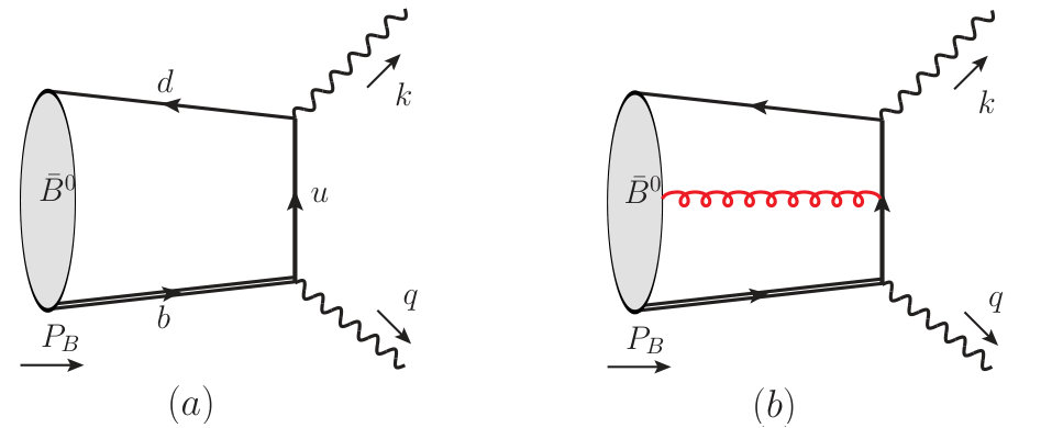 Figure 1
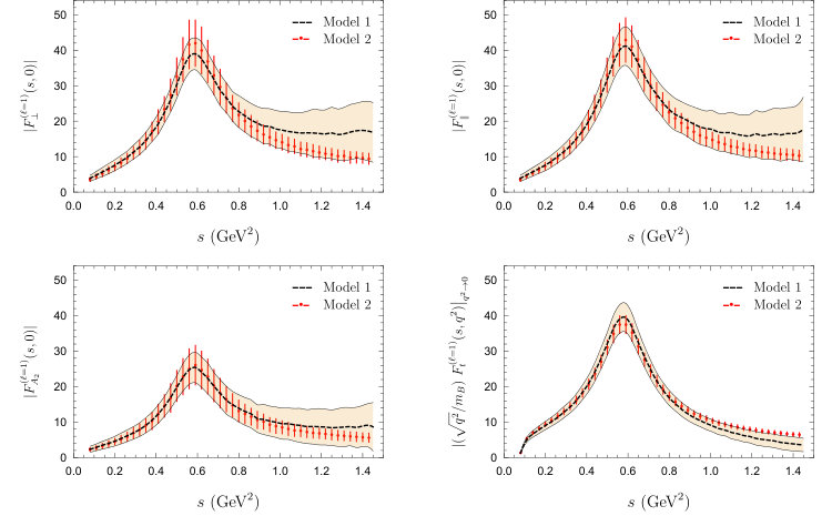 Figure 2
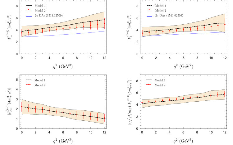 Figure 3
| correlation | + | + | + | + |
| correlation | + | + | + | + | ||||||||||||
| Resonance | (MeV) | (MeV) | weight factor |
|---|---|---|---|
| 1.0 | |||
Peer Reviews
No public reviews on file for this paper yet. If you reviewed it on a platform where reviews are public (OpenReview, ICLR, NeurIPS, ICML), you can paste yours below so the community can read it here.
Videos
No videos yet. Explain this paper in a talk, walkthrough, or lecture? Add one.
SI-HEP-2016-09
QFET-2016-04
NIOBE-2017-01
** Form Factors from Light-Cone Sum Rules
with -meson Distribution Amplitudes**
Shan Cheng, Alexander Khodjamirian and Javier Virto
a* Theoretische Physik 1, Naturwissenschaftlich-Technische Fakultät,
Universität Siegen, 57068 Siegen, Germany
b Albert Einstein Center for Fundamental Physics, Institute for Theoretical Physics,
University of Bern, CH-3012 Bern, Switzerland. *
Abstract
We study form factors using QCD light-cone sum rules with -meson distribution amplitudes. These form factors describe the semileptonic decay , and constitute an essential input in and decays. We employ the correlation functions where a dipion isospin-one state is interpolated by the vector light-quark current. We obtain sum rules where convolutions of the -wave form factors with the timelike pion vector form factor are related to universal -meson distribution amplitudes. These sum rules are valid in the kinematic regime where the dipion state has a large energy and a low invariant mass, and reproduce analytically the known light-cone sum rules for form factors in the limit of -dominance and zero width, thus providing a systematics for so far unaccounted corrections to transitions. Using data for the pion vector form factor, we estimate finite-width effects and the contribution of excited -resonances to the form factors. We find that these contributions amount up to in the small dipion mass region where they can be effectively regarded as a nonresonant (-wave) background to the transition.
Contents
1 Introduction
The transition form factors encode the rich hadronic dynamics accompanying the short-distance transition in the semileptonic () decays (see e.g. [1, 2]), which may provide a competitive determination of the CKM parameter [3] if an accurate knowledge of the form factors can be assessed. The form factors are also an essential hadronic input to the rare flavor-changing neutral-current decay [4] and to nonleptonic three-body decays such as [5, 6].
While form factors are dominated by the resonant transition (which has been studied extensively in the narrow-width approximation), finite-width effects and “nonresonant” contributions have not yet been addressed systematically. These effects are considerably more difficult to describe theoretically, providing non-trivial challenges for both analytical methods and lattice simulations. At large dipion invariant masses, the form factors can be calculated in QCD factorization [7]. For small dipion masses at low hadronic recoil, heavy-meson chiral perturbation theory may be combined with dispersion theory as proposed in Ref. [2]. At large hadronic recoil (and low dipion invariant mass), the method of light-cone sum rules (LCSRs) is operative, and has been used in Ref. [8] in terms of dipion distribution amplitudes (DAs) [9, 10]. However, the limited knowledge of these DAs asks for other QCD based methods to access the form factors in the same kinematic regime.
In this paper we propose to use the LCSRs with -meson DAs [11, 12, 13]. For definiteness we will focus on the transition with the isospin-one final dipion state; in the future these sum rules can be easily extended to the other isospin states. We will obtain a set of sum rules where the hadronic representation contains the form factors of interest convoluted with the timelike pion vector form factor. The latter is very accurately measured within a wide range of dipion masses. The sum rules obtained in this paper reproduce the known sum rules for the form factors in the limit of -dominance and zero width, and can be used to test models for form factors. We will illustrate this point by performing a numerical study of the effects of excited -resonances within a three-resonance model that fits the pion form factor accurately, assessing the deviations from -meson dominance in transitions.
The plan of the paper is the following. In Section 2 we derive the LCSRs with -meson DAs for the full set of vector and axial-vector form factors. The current accuracy of the operator-product expansion (OPE) includes the contributions of two- and three-particle DAs. In Section 3 we adopt a model for form factors in terms of -resonances. The LCSRs are then rewritten in the form of relations containing the model parameters. These relations are analyzed numerically in Section 4, taking as input a similar model for the pion vector form factor, fitted to the experimental data on . This analysis will allow us to quantify the deviations from the dominance approximation. We conclude in Section 5. The appendices contain: (A) the relevant formulae for -meson DAs used in LCSRs, (B) the model for the pion timelike form factor, and (C) the two-point sum rule used to fix the effective threshold in the sum rules.
2 Light-Cone Sum Rules
Following Ref. [12] we introduce the correlation function of the interpolation current with the weak current:
[TABLE]
sandwiched between the on-shell -meson and vacuum states. The four-momenta of the currents are and respectively, so that . The correlation function (1) is decomposed into independent Lorentz structures:
[TABLE]
where the first term 111 In this paper we use the conventions and . corresponds to the contribution of the vector current. Only the structures in the first line will be used in the sum rules below.
In the region and , due to the large virtuality of the intermediate -quark, the correlation function is calculable by means of an OPE, involving the DAs of the -meson defined in HQET. To leading order, one contracts the -quark fields in (1) as a free propagator, neglecting hereafter the -quark mass. The remaining heavy-light bilocal quark-antiquark operators sandwiched between the -meson and vacuum states are parametrized by the two-particle DAs , where is related to the momentum of the light-quark in the meson. We will also include the corrections due to a low virtuality (“soft”) gluon emitted from the propagator and absorbed in the three-particle -meson DAs [12]. The diagrams corresponding to the two contributions to the correlation function are shown in Fig. 1. The definitions of the DAs are listed in Appendix A together with the models we will use to describe them.
To outline the derivation of the sum rule, we choose the invariant amplitude , for which the corresponding OPE result can be written as
[TABLE]
where
[TABLE]
and the ellipsis denotes the subleading 3-particle DA contributions calculated in Ref. [12]. The OPE expression (3) has the form of a dispersion integral in the variable :
[TABLE]
with the imaginary part given by
[TABLE]
where is obtained by solving Eq. (4).
In parallel, for the same invariant amplitude we employ the hadronic dispersion relation in the variable ,
[TABLE]
The hadronic spectral function of the correlation function is obtained from the unitarity relation, that is, inserting the complete set of states with quantum numbers of the current between the two currents in Eq. (1):
[TABLE]
where the lowest intermediate dipion state is included explicitly and the ellipsis denotes the contributions from other intermediate states with higher thresholds: , etc. This hadronic representation is more general than the single-pole approximation adopted in Ref. [12], where the two-pion-state contribution was replaced by a single narrow -meson state.
We use the definition of the pion vector form factor:
[TABLE]
where and . In the isospin symmetry limit , where the pion electromagnetic form factor is normalized as . We also adopt the following definition for the form factors: 222 See e.g. Ref. [1]. Here we use the phase convention of Ref. [8].
[TABLE]
where is the kinematic Källén function. In addition, and
[TABLE]
where , and is the angle between the 3-momenta of the neutral pion and the -meson in the dipion rest frame. Note that the form factor in the decomposition of Eq. (10) parametrizes the transition matrix element of the vector weak current, whereas the other three form factors correspond to the axial-vector weak current.
For the form factors in Eq. (10) we will use the partial wave expansions
[TABLE]
where and are the associated Legendre polynomials. Only the -wave components shown explicitly in the above expansions survive in the convolution of the two hadronic matrix elements in Eq. (8). Indeed, the hadronic matrix element of the local current parametrized with the pion vector form factor contains only the -wave dipion contribution and hence effectively serves as a -wave projector for the form factors. In order to extend the method suggested here to other partial waves one needs to replace the interpolating current in the correlation function with a different current or combination of currents.
Substituting the definitions (9) and (10) in Eq.(8), integrating over the angles in the dipion phase space and sorting out the different kinematic structures, we obtain the imaginary parts of all relevant invariant amplitudes. In particular, the one generated by the vector current reads:
[TABLE]
where hereafter and again the ellipsis denote contributions from the intermediate states , etc. Judging by studies on pion form factors at , these contributions are expected to be suppressed (see e.g. Ref. [14] and the discussion in Ref. [2]).
We then insert the hadronic spectral function (13) in the r.h.s. of Eq. (7). For the l.h.s. we use Eq. (5), as the OPE is a good approximation to the correlation function in the region . At this point, we Borel-transform both sides of the resulting equality, effectively replacing the variable with the Borel parameter squared . In addition, we employ the quark-hadron duality approximation, which amounts to the assumption that the integrals over the hadronic spectral density and over are equal:
[TABLE]
where is the effective threshold. The above semi-local duality relation allows one to effectively cut-off the integrals over the dipion mass in the sum rule. Note that we use a quark-hadron duality ansatz, which is more general than a local duality, that would assume equality of the integrands on both sides of Eq. (14) for every . Note also that the falling Borel exponent (provided is not too large) suppresses the large region of the integrals, making the duality relation less sensitive to multihadron states with thresholds larger than . Depending on the choice of , the and states may still contribute to the region but their expected suppression with respect to the dipion state justifies to retain only the latter in .
Finally, we obtain the following LCSR:
[TABLE]
where is the solution of the relation and the explicit expression for the three-particle DA contribution can be found in the Appendix of Ref. [12].333 Note that the factor has to be removed from the integrand.
Repeating the same steps for the invariant amplitudes and in Eq. (2), we obtain two additional LCSRs containing the integrals over the form factors and respectively:
[TABLE]
and
[TABLE]
where is defined in Appendix A, and the three-particle contributions can be again found in the Appendix of Ref. [12].3
The remaining Lorentz structures in the correlation function provide additional, more complicated relations between the three form factors, hence we do not consider them here. Instead, we obtain a new sum rule for the “timelike-helicity” form factor by considering a different correlation function with the pseudoscalar heavy-light current,
[TABLE]
The form factor can be isolated by multiplying both sides of Eq. (10) with , giving
[TABLE]
After inserting the dipion intermediate state in Eq. (18), only the above form factor contributes. Considering the invariant amplitude and carrying out a similar derivation as for the previous correlation function, we obtain the following LCSR for :
[TABLE]
where the OPE result in the r.h.s. is new and has not been given before. The new expression for the three-particle contribution is given explicitly in Appendix A.
The sum rules in Eqs. (15)-(17) and (2) with generalized hadronic part represent the main results of this paper. They provide additional constraints and normalization for form factors if one adopts a certain ansatz or model for them. On the other hand, if the form factors are calculated via an alternative method, one can check the validity and consistency of the results. In addition to the universal -meson DAs, the pion vector form factor in the timelike region represents the necessary input in these sum rules. The magnitude of this form factor is well known experimentally from [15] and [16].
Our last comment in this section concerns the final state interaction phase. Below the inelastic threshold for the pion form factor this phase coincides with the dipion elastic scattering phase according to Watson’s theorem. Here an analogous condition should be fulfilled in the adopted approximation of two-pion intermediate state in the hadronic dispersion relation. Due to the reality of the imaginary parts, such as the one in Eq. (13), the strong phase of all form factors should be universal (modulo ) and equal to the phase of the pion vector form factor:
[TABLE]
This condition was already mentioned and used in the elastic scattering region in Ref. [2].
Note that since Eq. (21) follows from the general unitarity relation, it enforces any parametrization of the form factors to be chosen such that the phases of separate -dependent components in each form factor can only depend on , being correlated with the phase of the pion form factor. In the following we will take this condition into account when choosing a particular ansatz for the form factors.
3 Probing resonance models for form factors
Originally, the LCSRs with -meson DAs derived from the correlation function in Eq. (1) were used in Ref. [12] to determine the form factors. In what follows we use the standard definition of these form factors:
[TABLE]
where .
To recover the sum rules obtained in Ref. [12] from the sum rules derived in the previous section, one has to employ the dispersion relation in for the form factors retaining only the single -pole contribution. E.g., for the vector-current form factor one has:
[TABLE]
where the excited state contributions with the quantum numbers indicated by the ellipsis are assumed to be accounted for by the duality approximation. Note that in the above, for the sake of generality, we go beyond the narrow approximation and adopt the energy-dependent width
[TABLE]
so that is the total width and the function vanishes below the dipion threshold . The energy-dependent width can be interpreted as a result of the resummation of two-pion loops coupled to the state. For consistency, a -dominance approximation for the pion form factor has to be adopted too:
[TABLE]
where the -meson decay constant and strong coupling are normalized as:
[TABLE]
Using the approximations of Eqs. (23) and (25) and taking into account Eq. (24), the l.h.s. of Eq. (15) becomes
[TABLE]
where we have used that in the zero-width limit (), the expression in parentheses reduces to . Thus, we recover the LCSR for the form factor obtained in Ref. [12]. Analogously, starting from Eqs. (16), (17) and (2) we recover the LCSRs for the form factors and respectively.
We note at this point that relating the form factor with the form factors according to the relation quoted after Eq. (22), and using the kinematic relation , we obtain an alternative sum rule for . This sum rule coincides with Eq. (27) up to power corrections, with , i.e., within the usual accuracy of the LCSRs with -meson DAs [12]. Thus our sum rule for satisfies the kinematic relation up to power corrections.
Returning to the LCSRs in Eqs. (15)-(17) and (2) with a general hadronic representation of the dipion state, we note that these sum rules offer the opportunity to go beyond the -dominance approximation and to investigate the role of excited resonances in form factors. From the measurements of the pion e.m. form factor in annihilation (see e.g. Ref [16]) and the pion vector form factor in [15], it is known that in the region both form factors are accurately described by including, apart from the , its two radial excitations: and [17]. In what follows, we adopt the three-resonance parametrization of used by the Belle collaboration [15] to fit their so far most accurate data on (see Appendix B). Various other parametrizations for the pion form factors in the timelike region can be found in the literature (see e.g. [18, 19, 21, 20, 22]). The important point is that, at least in the low dipion-mass region, the “nonresonant” contributions can be described well by the interference of the with the and , and these excited states contribute at the level of to the total form factor 444 Note that at larger the infinite tail of vector resonances may influence the form factor and it presumably has to be taken into account [23, 18, 19]. .
Assuming that the formation and hierarchy of -resonances in the transition is similar to that in , we adopt a three-resonance ansatz generalizing Eq. (23) for all vector and axial-vector -wave form factors. For the form factors and we write 555 For the sake of generality, we include also the relative phase of the term. :
[TABLE]
where the sum runs over . The linear combination of and entering the LCSR in Eq. (17) is related to the form factors :
[TABLE]
Finally, for the form factor , we have
[TABLE]
For our exploratory study we refrain from using the more involved resonance representation of Ref. [24], adopting instead a simpler Breit-Wigner approximation with an energy-dependent width [25]. We also tacitly assume that the phase factors of resonance contributions are independent of the form factor type. On the other hand, it is conceivable that -dependence of the form factors is different for . Hence the simplest way to enforce the imaginary part condition of Eq. (21) is to assume that this condition holds separately for each resonance term in the models of Eqs. (28)-(31). Then the phase is -dependent but -independent, and the general condition (21) is replaced with the following relation specific to our resonance model:
[TABLE]
This relation essentially restricts the resulting phase dependence of the form factors, in full analogy with the well-known situation for the timelike pion form factor. Adopting a more general condition than Eq. (32), would enforce an artifitial compensation of -dependences in the phases and form factors, in order to formally obey Eq. (21). Moreover, there are several physical arguments in favour of -independent phases of form factors in the region of dipions with large recoil and small invariant mass. First, varying corresponds to varying the total energy of the dipion state, produced in the -meson rest frame, whereas the (Lorentz-invariant) amplitude of the final-state strong interaction developing the phase depends only on the invariant mass of the dipion. Second, similar to the factorization in nonleptonic -decays to light hadrons, the hadronization and related strong interaction of the fast dipion system in the -meson rest frame takes place beyond the weak transition domain.
We parametrize the -dependence of the form factors entering Eqs. (28)-(31) with the standard -series expansion [26], in the form adopted in Ref. [27]. The -parametrization of the momentum transfer is given by
[TABLE]
where and . For a generic form factor , where and , we have:
[TABLE]
where we use the shorthand notation
[TABLE]
and is the lowest heavy-light pole mass in the channel with spin-parity depending on the type of the form factor.
We now substitute the resonance models of Eqs. (28)-(31) into the sum rules (15)-(17) and (2) respectively. For the sake of brevity we introduce the following notation:
[TABLE]
so that all four sum rules can be rewritten in a generic form:
[TABLE]
In the above, the functions with represent the r.h.s of Eqs. (15)-(17) and (2) respectively and the coefficients of the form factors are given by the integrals:
[TABLE]
The set of sum rule relations (36) can be used to fit the parameters and of the resonance models in Eqs. (28)-(31) for the form factors.
4 Input and numerical analysis
The input in the LCSRs (15)-(17) and (2) includes the parameters of -meson DAs described in Appendix A. The most important one is the inverse moment , which has still a rather large uncertainty. The interval
[TABLE]
predicted from QCD sum rules [28], is in agreement with the lower limit MeV (at C.L.) recently obtained by the Belle collaboration [31], combining the search for with the theory prediction for its branching ratio [32, 33]. This limit is starting to challenge the lower values around MeV preferred by the QCD factorization analysis of nonleptonic decays (see e.g., Refs. [29, 30]). In addition, a recent estimate MeV [34] has been obtained by comparing the LCSRs with pion [35] and -meson DAs for the form factor and using the same model for the -meson DA as the one used here. In our numerical analysis we adopt the central value and uncertainty of the sum rule prediction quoted in Eq. (38).
Since we do not include NLO corrections in the correlation functions, we also do not take into account the renormalization of . In the absence of perturbative corrections, the choice of renormalization scale for the correlation function remains an open issue. This choice concerns especially the sum rule (2) for which the -quark mass is needed. We choose a typical value . The value of the (scale-independent) -meson decay constant entering the OPE part of all LCSRs is known with a reasonable accuracy from the 2-point QCD sum rules. We use MeV from Ref. [36], which agrees well with lattice QCD determinations [37].
For the Borel parameter in all the sum rules we take values inside the interval , which is slightly narrower than the one used in Ref. [11]. For this interval, the convergence of OPE is manifested by relatively small three-particle DA contributions (with at and at ). Simultaneously, the integral over the spectral density of the correlation function (r.h.s. of Eq. (14)) does not exceed 40% of the total integral, making the result not too sensitive to the quark-hadron duality approximation.
The choice of the threshold parameter deserves a separate investigation. We emphasize that here a quark-hadron duality pattern is used that is more involved than the conventional one-pole-plus-continuum ansatz. Hence, for consistency we fix the threshold employing the two-point SVZ sum rule [38] for the isospin-one light-quark vector currents, where we substitute the pion timelike form factor in the hadronic part. The details are given in Appendix C. The result depends mildly on the value of the Borel parameter , and within our chosen range it leads to quite generically, in the same ballpark as the one obtained with the one-pole ansatz.
The remaining input concerns the hadronic parameters in Eq. (37). For the pion form factor we use the model of Ref. [15] and the fit results for its parameters given in that paper, which are collected in Appendix B for convenience. These include determinations for and appearing explicitly in Eq. (37). For the pole masses in Eqs. (34) and (36), we use [17]:
[TABLE]
After specifying all input parameters, we calculate the coefficients and in Eq. (36). In order to have an impression on the relative contributions of all three resonances to the sum rule relations (36) we quote the values of the coefficients , varying the values for all masses, widths, and the parameters in as given in Table 4:
[TABLE]
calculated at GeV2 and GeV2. We also quote here the value of the strong coupling derived from Eq. (24):
[TABLE]
which is necessary to relate the coefficients to the form factors . In the following we will consider all uncertainties entering , but fix the hadronic parameters entering and to their central values.
4.1 Finite-width effects in form factors
We start our numerical analysis reproducing the results of Ref. [12] for the form factors by taking the one-pole ansatz for the form factors, i.e. retaining only the in Eqs. (28)-(31) in the narrow width approximation, and subsequently taking into account the corrections arising from the finite width of the and the effect from higher resonances (acting effectively as a “nonresonant” background). We do this in several steps, with the results summarized in Table 1:
Employing the one-resonance models in Eqs. (23), (25) – and the analogous models for – in the limit , we use the sum rules to calculate the form factors and at . With the same inputs as used in Ref. [12] we find good agreement with the central values quoted in that paper666 The form factor was not calculated in Ref. [12]. Thus the results for given here are new. . These numbers are collected in the first row of Table 1. Updating the input parameters to the ones quoted at the beginning of this section (but still keeping fixed), we find a enhancement in the central values, due mostly to the change in the numerical input for the -meson decay constant: (second row of Table 1). Performing a gaussian scan over the parameters with uncertainties, we calculate central values and errors for the form factors by taking the mean and standard deviation of the resulting distributions for the form factors (third row of Table 1). This shifts the central values further up slightly (but well within the uncertainties). The larger error bars with respect to Ref. [12] are due to the different approach used here (gaussian versus flat scans). These are our results in the single-pole approximation (-dominance, zero-width). For reference we show in the fourth row in Table 1 the results for the form factors obtained in Ref. [39] (updating Ref. [40]) using the LCSRs with -meson DAs, in which the zero-width approximation is also adopted.
We now maintain the one-resonance model for the form factors, but adopt the full Belle [15] data-based model for (see Appendix B). Keeping , we obtain the results quoted in the fourth row of Table 1, which imply a enhancement with respect to the zero-width limit. Our final results for the single resonance model are obtained by simultaneously fitting the sum rules with different values of the Borel parameter . The results are given in the last row of Table 1. The central values are essentially unchanged, but the uncertainties are reduced because each value of acts as a separate constraint.
We conclude that the finite width of the and the presence of higher resonances in impact the form factors at the level of , when the form factors are defined from the form factors by neglecting the contributions from excited resonances in Eqs. (28)-(31). This is in agreement with the findings in Ref. [8].
4.2 Assessing the contribution to form factors
In order to estimate the contribution, we now assume that the form factors are well determined from the LCSRs with -meson DAs, obtained in the narrow- approximation. We thus take the models in Eqs. (28)-(31), neglecting the contribution, and use the results from Ref. [39] to fix the parameters and . The free parameters in the resulting models are then only and .
We then use the sum rules (15)-(17) and (2) to determine these parameters. Besides using, as in the previous section, three different values for the Borel parameter , we consider various points: , in order to determine the slope parameters . The results of this fit are shown in Table 2. Due to the suppressed sensitivity of the sum rules to the region (see Eq. (40)), the uncertainties on the parameters and are rather large. Thus our fit allows for a quite appreciable contribution relative to the (fixed) contribution.
4.3 Three-resonance model
We now consider the full three-resonance models given in Eqs. (28)-(31). This model however contains too many parameters to be independently fitted from the sum rules, in which the contributions of enter with suppressed coefficients with respect to the contribution (see Eq. (40)). In the future, when sufficient amount of data on is accumulated, one should be able to isolate the -wave dipions in this decay and perform a more refined analysis combining these data with the sum rule constraints. For the time being, the only information on the role of higher resonances we have is provided by the measurement given by the parametrization in Eq.(55). Note that in the pion vector form factor the -resonance () contribution is determined by the product of the decay constant of and the strong coupling , whereas in the form factor the -contribution to the resonance model is determined by the form factor multiplied by the coupling . Owing to quite different physical processes, the ratios of form factors may deviate considerably from the ratios of decay constants. E.g., it is plausible that at large recoil the transition is even enhanced with respect to transition because the hadronization into a larger mass is more probable. Nevertheless, since in this paper we want to illustrate numerically the influence of the nonresonant background in the transitions at small dipion mass, it is conceivable to assume that the relative size of the contributions from and is the same as in . We do that by imposing the following conditions:
[TABLE]
where and are the parameters in the parametrization of in Eq. (54). The conditions on fix the relative contributions at and the conditions on fix the derivatives. At the end we find that the conditions (42) fix the relative contributions in the full region with good accuracy.
These simplified models depend only on two parameters for each form factor: and . We use the sum rules to determine these parameters, using again the three values of , and also . The results of the fit are given in Table 3. We note that the values for and are strongly correlated within each form factor, with correlation coefficients given in the third row. We provide for completeness also the resulting form factors at and the values of the parameters and for , although all these numbers can be obtained rather trivially from the first three rows.
Given the fact that the and contributions to the pion form factor are relatively small, the results of the form factors obtained in the constrained three-resonance model are in good agreement with the ones obtained in the -model (compare the third row in Table 3 with the fifth row in Table 1). The effect of the higher resonances is to decrease slightly the form factors. The uncertainties obtained in this section are smaller only because the fit includes many points in the full region, all acting as separate (and consistent) constraints, while in Table 1 we only considered the form factors at .
In Fig 2 we show the results for the absolute values of the form factors, comparing the model results in Table 2 (Model 1) and Table 3 (Model 2). The results for depend on the correlations between and , and in order to ignore this correlation we plot instead defined as
[TABLE]
which at depends only on . There is good agreement between both models. Due to large uncertainties in , Model 1 yields broader intervals for the form factors at above the region. Larger form factors in this region are compensated by slightly smaller values around in order to satisfy the sum rules.
Within Model 1 (Table 2), the fitted intervals for form factors (albeit with very large uncertainties) do not exclude a noticeable (up to 20%) contribution of the transition to the total budget of the form factors at small dipion masses. In Model 2 (Table 3) where the relatively small (most probably underestimated) contributions of both and are fixed, the resulting form factor grows insignificantly with respect to the one in Model 1, staying within the estimated uncertainties of the latter. We conclude that the LCSRs with meson DAs provide a stable prediction for the dominant part of the -wave form factors, provided the component remains bounded. The transitions to excited -mesons, being subdominant in the sum rules, cannot be predicted with a high degree of accuracy unless one adopts some particular ansatz for their pattern. At the same time a sizeable contribution from excited states is consistent with our LCSRs, and is supported by the independent LCSRs in terms of dipion DAs considered in Ref. [8]. Hence, in the future, more precise measurements of form factors must include these contributions with interfering phases in their fits. This is a necessary step in accurately determining the form factors. Restricting the dipion mass in the -mass region, as it is usually done (see e.g. Ref. [3]), is not sufficient if an accuracy better than 15-20% is sought.
We finish this section with a brief discussion on the dependence of the form factors, and comparing our results to the ones obtained in Ref. [8]. This is shown in Fig. 3. We find that our results are compatible with the results of Ref. [8] for , with the absolute magnitude of the latter a bit below our results. The calculation of in terms of dipion DAs is still work in progress (only a relationship between , and is given in Ref. [8]), and thus we cannot perform such comparison for and . Our results for the slope parameters have a significant error, and thus one would naively expect that the uncertainties in the form factors increase visibly with , contrary to what is seen in Fig. 3 where the uncertainties are rather constant. The reason for this is the large positive correlation between and (of around , see Tables 2 and 3). Since is negative, lower values of (corresponding to lower values of the form factors at ) are correlated with lower values of (corresponding to larger slopes for the form factors and larger values at ), and viceversa.
5 Conclusions
In this paper we have suggested a new approach to the transition form factors in the region of small dipion mass, employing the LCSRs with -meson DAs. We have focused on the particular transition, generated by the weak current, with an isospin-one and -wave dipion final state. The fact that this state is interpolated by the light-quark vector current allows one to go beyond the single narrow -meson approximation, probing also the contributions of other intermediate states with the same quantum numbers. We have obtained the LCSRs in a general form in which the convolutions of -wave form factors with the pion vector form factor integrated over the quark-hadron duality interval are related to the integrals over -meson DAs. The latter are calculated from the OPE of the underlying correlation function, taking into account the two- and three-particle -meson DAs and reproducing the results obtained earlier in Refs. [11, 12]. In addition, we have derived a new sum rule for the form factor starting from a slightly modified correlation function and including the three-particle contribution , which is given here explicitly for the first time (see Appendix A).
We have performed an exploratory numerical analysis using as an input the vector form factor measured by the Belle collaboration, and fitted in a form of a superposition of three resonances. We have then investigated the impact of the nonresonant and excited states on the sum-rule results for the dominant form factor, including the effects of the total width of , and of the excited resonance contributions to the vector form factor. Using an independent calculation of form factors from LCSRs with zero-width -meson DAs, we find that the contributions from and other states in the region of low dipion mass can be typically at the level of 15-20%. This is consistent with the results of Ref. [8] based on LCSRs for form factors in terms of dipion DAs. Hence, the combination of these two independent methods (LCSRs with dipion or -meson distribution amplitudes) can be used in the future for reciprocal tests of the results.
Further development of the approach suggested in this paper is foreseeable in several directions. First, the accuracy of the OPE can be improved further, by calculating the perturbative NLO corrections and pinning down the uncertainty in the parameters of the meson DAs. Second, the description of the pion vector form factor and probably also of the of form factors in the small dipion mass region can be implemented in a more model-independent fashion employing the dispersion approach and the Omnès representation in the spirit of Ref. [2], that is, with no explicit resonance ansatz. Finally, the method can be extended to other form factors with and with various spin-parities and flavor combinations, for example to form factors.
One of the necessary requirements to improve on the accuracy of the observable-rich exclusive -decays with unstable mesons in the final states (such as , or ) is a reliable and maximally comprehensive description of the nonresonant background stemming from excited and continuum states. Such a description should already begin at the stage of fitting the data, and the general or form factors, respectively, should serve as a starting point. The sum rules considered in this paper provide a useful theoretical tool for such purpose. Our analysis is a first step towards a coherent approach to decays into unstable hadrons.
Acknowledgments
We are grateful to G. Colangelo, S. Descotes-Genon, L. Tunstall, D. van Dyk, Y.M. Wang and W.F. Wang for discussions and comments. This work is supported by the DFG Research Unit FOR 1873 “Quark Flavour Physics and Effective Theories”, contract No KH 205/2-2. J.V. acknowledges funding from the Swiss National Science Foundation, from Explora project FPA2014-61478-EXP, and from the European Union’s Horizon 2020 research and innovation programme under the Marie Sklodowska-Curie grant agreement No 700525 ‘NIOBE’.
Appendix A -meson Distribution Amplitudes
We use the standard definition of the two-particle -meson DAs in the momentum representation[41, 42]:
[TABLE]
where is the gauge factor and the meson state with four velocity is defined in HQET. We retain the relativistic normalization up to corrections; also the quark field is replaced by the effective field using . The variable is the plus component of the light-quark momentum in the meson. We also use the notation:
[TABLE]
The four three-particle DAs emerge in the decomposition of the quark-antiquark-gluon matrix element (see Ref. [12] for details):
[TABLE]
where the path-ordered gauge factors in the l.h.s. are omitted for brevity. The DA’s ,, and depend on and being, respectively, the plus components of the light-quark and gluon momenta in the meson.
In the numerical analysis we adopt the popular exponential model [41] of the -meson two-particle DAs:
[TABLE]
where the parameter is equal to the inverse moment , defined as
[TABLE]
We also use the related models for the three-particle DAs developed in Ref. [12]:
[TABLE]
where is adopted. The three-particle contributions to the sum rules and can be found in Ref. [12]. However, the expression for has not yet been given in the literature. In complete analogy with the calculation of Ref. [12], we find:
[TABLE]
where
[TABLE]
and the integrals over the three-particle DA’s multiplying the inverse powers of the Borel parameter with are defined as:
[TABLE]
where:
[TABLE]
The non-vanishing coefficients entering Eq. (51) are given by:
[TABLE]
Appendix B The pion timelike form factor
We use the results for the pion vector form factor obtained from the measurement of decay by Belle Collaboration [15] and fitted to the combination of three -resonances, for which the Gounaris-Sakurai model [24] was adopted
[TABLE]
where
[TABLE]
and the functions and entering the resonance model are not shown here for the sake of brevity and can be found e.g., in Eqs. (14)-(16) of [15], so that . (For a simple derivation of the GS model see e.g., [18].) Furthermore, we use the parameters of the constrained fit () taken from the Table VII of Ref. [15], which we reproduce in Table 4. We also note that the masses of resonances and their total widths are in a good agreement with the averages in [17].
Appendix C Fixing the effective threshold
We employ the QCD (SVZ) sum rules [38] for the two-point correlation function:
[TABLE]
where the lowest two-pion contribution to the hadronic spectral density is written in a general form, proportional to the square of the pion vector form factor:
[TABLE]
It is easy to check that replacing the form factor by the single approximation in the zero-width limit , brings this expression to the familiar form . Furthermore, we substitute in eq.(57) the measured form factor squared and calculate numerically the integral over Im weighted with the Borel exponent:
[TABLE]
The above integral is equated to the Borel-transformed correlation function calculated in QCD and containing the perturbative loop contribution (to NLO) and the vacuum condensate terms (up to ):
[TABLE]
where
[TABLE]
is the compact notation for the contributions from dimension-4 (quark and gluon) and dimension-6 (four-quark) condensates, respectively. In the above expressions the quark-condensate contribution is related to the pion decay constant MeV and the input parameters are: [17], [43, 17] and [44].
Fitting the integral to its QCD sum rule counterpart we find the following values depending on the Borel parameter:
[TABLE]
which is close to the duality interval in the original SVZ sum rule [38] for the meson.
The reference list from the paper itself. Each links out to its DOI / PubMed record.
- 1[1] S. Faller, T. Feldmann, A. Khodjamirian, T. Mannel and D. van Dyk, “Disentangling the Decay Observables in B − → π + π − ℓ − ν ¯ ℓ → superscript 𝐵 superscript 𝜋 superscript 𝜋 superscript ℓ subscript ¯ 𝜈 ℓ B^{-}\to\pi^{+}\pi^{-}\ell^{-}\bar{\nu}_{\ell} ,” Phys. Rev. D 89 , 014015 (2014) [ar Xiv:1310.6660 [hep-ph]].
- 2[2] X. W. Kang, B. Kubis, C. Hanhart and U. G. Meißner, “ B l 4 subscript 𝐵 𝑙 4 B_{l 4} decays and the extraction of | V u b | subscript 𝑉 𝑢 𝑏 |V_{ub}| ,” Phys. Rev. D 89 , 053015 (2014), [ar Xiv:1312.1193 [hep-ph]].
- 3[3] Belle collaboration, “Study of Exclusive B → X u ℓ ν → 𝐵 subscript 𝑋 𝑢 ℓ 𝜈 B\to X_{u}\ell\nu Decays and Extraction of | V u b | subscript 𝑉 𝑢 𝑏 |V_{ub}| using Full Reconstruction Tagging at the Belle Experiment,” Phys. Rev. D 88 , no. 3, 032005 (2013) [ar Xiv:1306.2781 [hep-ex]].
- 4[4] LH Cb collaboration, “Study of the rare B s 0 superscript subscript 𝐵 𝑠 0 B_{s}^{0} and B 0 superscript 𝐵 0 B^{0} decays into the π + π − μ + μ − superscript 𝜋 superscript 𝜋 superscript 𝜇 superscript 𝜇 \pi^{+}\pi^{-}\mu^{+}\mu^{-} final state,” Phys. Lett. B 743 , 46 (2015) [ar Xiv:1412.6433 [hep-ex]].
- 5[5] S. Kränkl, T. Mannel and J. Virto, “Three-Body Non-Leptonic B Decays and QCD Factorization,” Nucl. Phys. B 899 , 247 (2015), [ar Xiv:1505.04111 [hep-ph]].
- 6[6] J. Virto, “Charmless Non-Leptonic Multi-Body B decays,” Po S FPCP 2016 , 007 (2016), ar Xiv:1609.07430 [hep-ph].
- 7[7] P. Böer, T. Feldmann and D. van Dyk, “QCD Factorization Theorem for B → π π ℓ ν → 𝐵 𝜋 𝜋 ℓ 𝜈 B\to\pi\pi\ell\nu Decays at Large Dipion Masses,” ar Xiv:1608.07127 [hep-ph]
- 8[8] C. Hambrock and A. Khodjamirian, “Form factors in B ¯ 0 → π π ℓ ν ¯ ℓ → superscript ¯ 𝐵 0 𝜋 𝜋 ℓ subscript ¯ 𝜈 ℓ \bar{B}^{0}\to\pi\pi\ell\bar{\nu}_{\ell} from QCD light-cone sum rules,” Nucl. Phys. B 905 , 373 (2016), [ar Xiv:1511.02509 [hep-ph]].