Learning Sparse Structural Changes in High-dimensional Markov Networks: A Review on Methodologies and Theories
Song Liu, Kenji Fukumizu, Taiji Suzuki

TL;DR
This paper reviews methodologies for directly learning sparse structural changes in high-dimensional Markov Networks, emphasizing recent theoretical and practical advances in capturing system alterations efficiently.
Contribution
It provides a comprehensive review of direct change learning methods in Markov Networks, highlighting recent developments and theoretical insights.
Findings
Summarizes recent methodologies for sparse change detection.
Highlights theoretical guarantees for change learning.
Discusses practical applications and challenges.
Abstract
Recent years have seen an increasing popularity of learning the sparse \emph{changes} in Markov Networks. Changes in the structure of Markov Networks reflect alternations of interactions between random variables under different regimes and provide insights into the underlying system. While each individual network structure can be complicated and difficult to learn, the overall change from one network to another can be simple. This intuition gave birth to an approach that \emph{directly} learns the sparse changes without modelling and learning the individual (possibly dense) networks. In this paper, we review such a direct learning method with some latest developments along this line of research.
Click any figure to enlarge with its caption.
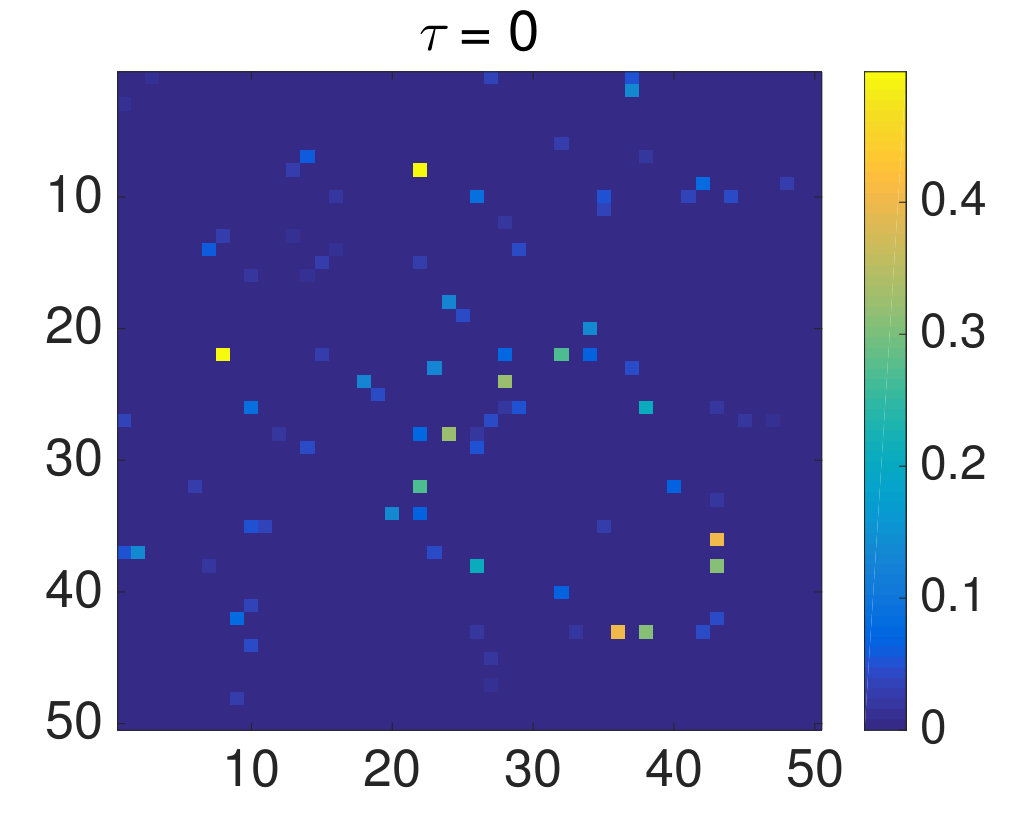 Figure 1
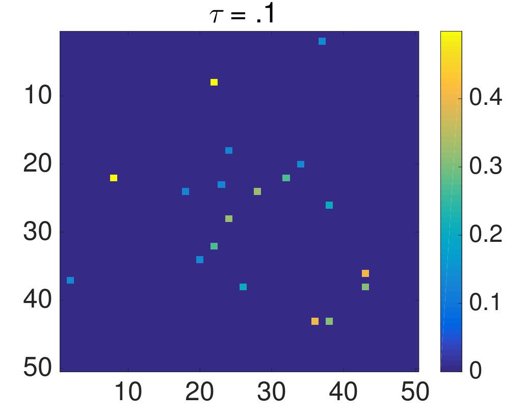 Figure 2
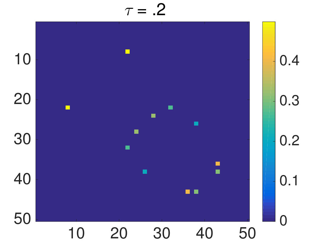 Figure 3
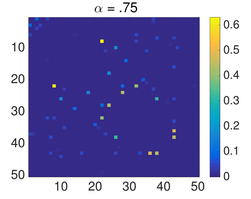 Figure 4
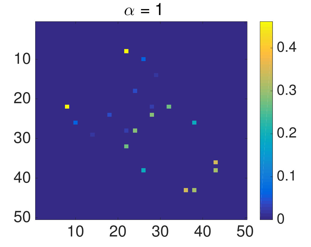 Figure 5
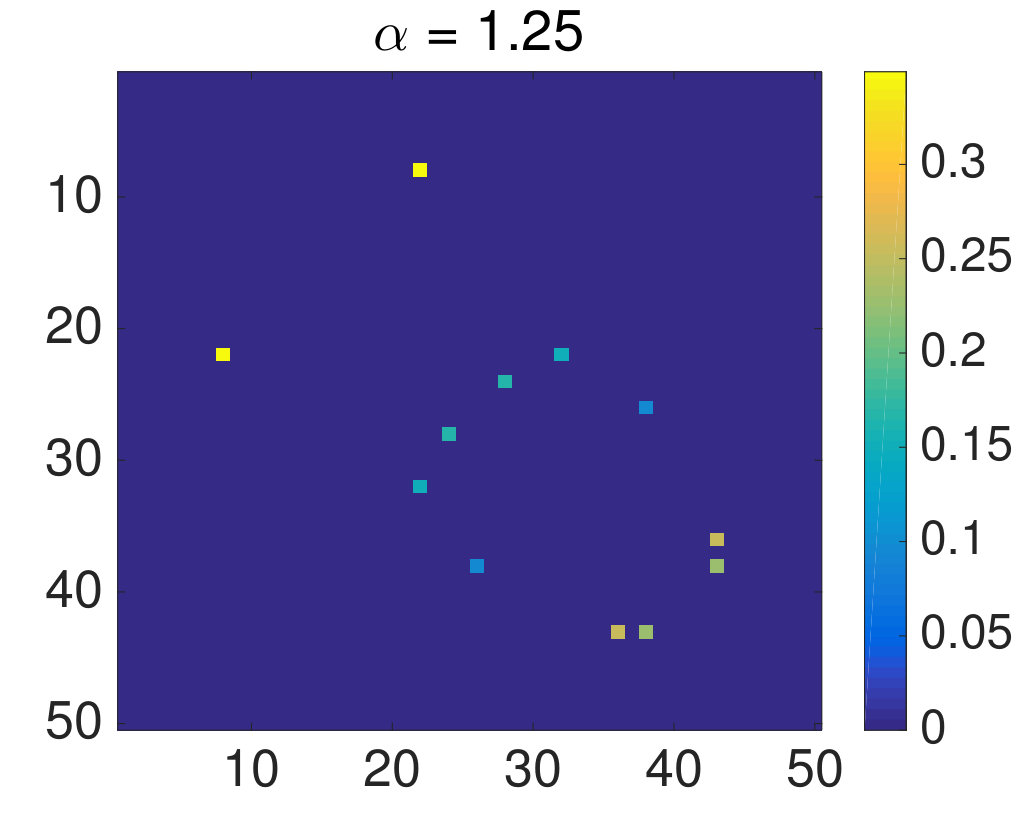 Figure 6
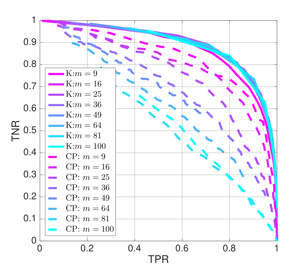 Figure 7
 Figure 8
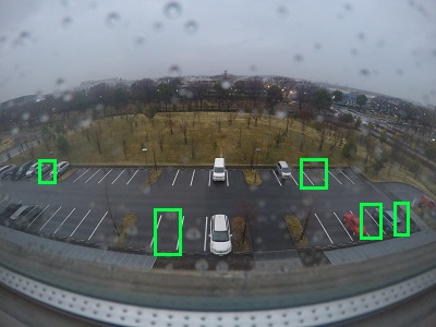 Figure 9
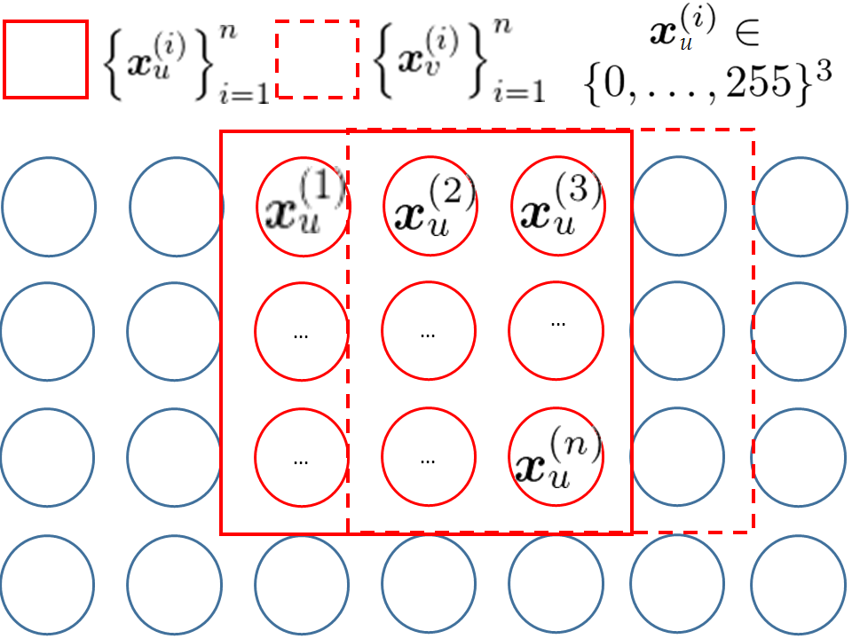 Figure 10
 Figure 11
 Figure 12
| K | 0.8746 | 0.8865 | 0.8899 | 0.8890 | 0.8902 | 0.8878 | 0.8903 | 0.8866 |
| CP | 0.8165 | 0.7917 | 0.7627 | 0.6829 | 0.5574 | 0.5914 | 0.5475 | 0.5656 |
Peer Reviews
No public reviews on file for this paper yet. If you reviewed it on a platform where reviews are public (OpenReview, ICLR, NeurIPS, ICML), you can paste yours below so the community can read it here.
Videos
No videos yet. Explain this paper in a talk, walkthrough, or lecture? Add one.
Taxonomy
TopicsAnomaly Detection Techniques and Applications · Machine Learning and Data Classification · Face and Expression Recognition
Learning Sparse Structural Changes in High-dimensional Markov Networks: A Review on Methodologies and Theories
Song Liu
Kenji Fukumizu
Taiji Suzuki
Song Liu
The Institute of Statistical Mathematics
10-3 Midori-cho, Tachikawa, Tokyo 190-8562, Japan
Kenji Fukumizu
The Institute of Statistical Mathematics
10-3 Midori-cho, Tachikawa, Tokyo 190-8562, Japan
Taiji Suzuki
Tokyo Institute of Technology
2 Chome-12-1 Ookayama, Meguro, Tokyo 152-8550, Japan
PRESTO, Japan Science and Technological Agency (JST), Japan
Abstract
Recent years have seen an increasing popularity of learning the sparse changes in Markov Networks. Changes in the structure of Markov Networks reflect alternations of interactions between random variables under different regimes and provide insights into the underlying system. While each individual network structure can be complicated and difficult to learn, the overall change from one network to another can be simple. This intuition gave birth to an approach that directly learns the sparse changes without modelling and learning the individual (possibly dense) networks. In this paper, we review such a direct learning method with some latest developments along this line of research.
1 Introduction
The problem of learning the changes of interactions between random variables can be useful in many applications. For example, genes may regulate each other in different ways when external conditions are changed; the number of daily flu-like symptom reports in nearby hospitals may become correlated when a major epidemic disease breaks out; EEG signals from different regions of the brain may be synchronized/desynchronized when the subject is performing different activities. Spotting such changes in interactions may provide key insights into the underlying system.
The interactions among random variables can be formulated as undirected probabilistic graphical models, or Markov Networks (MNs) (Koller and Friedman, 2009), expressing the interactions via the conditional independence. We consider a simple model: the pairwise MNs where the links are only encoded for single or pairs of random variables. Due to the Hammersley-Clifford theorem (Hammersley and Clifford, 1971), the underlying joint probability density function can be represented as the product of univariate and bivariate factors.
As an important challenge, structure learning of MNs has also attracted a significant amount of attention. Earlier methods (Spirtes et al., 2000) use hypothesis testing to learn the conditional independence among random variables, which reflects the absences of edges. It is proved that such a problem is generally NP-hard (Chickering, 1996). Methods restricted to a sub-class of graphical models (such as trees or forests) (Chow and Liu, 1968; Geman and Geman, 1984; Liu et al., 2011) also suffer from growing computational cost.
However, the Hammersley-Clifford theorem together with the recent breakthrough on sparsity-inducing methods (Tibshirani, 1996; Zhao and Yu, 2006; Wainwright, 2009) gave birth to many sparse structure learning ideas where the sparse factorization of the joint/conditional density function was estimated to infer the underlying structure of the MN (Friedman et al., 2008; Banerjee et al., 2008; Meinshausen and Bühlmann, 2006; Ravikumar et al., 2010). Although most works focused on parametric models, the structure learning has been conducted on semi-parametric ones in recent years. (Liu et al., 2009, 2012).
There is also a trend of learning the changes between MNs (Zhang and Wang, 2010; Liu et al., 2014; Zhao et al., 2014). Comparing to standard structure learning, the learning of changes views the problem in a more dynamic fashion: Instead of estimating a static pattern, we hope to obtain a dynamic one, namely “the change” by comparing two sets of data. Since in some applications, the static pattern may not be computationally tractable, or simply too hard to comprehend. However, the difference between two patterns may be represented by some simple incremental effects involving only a small number of nodes or bonds, Thus it takes much less effort to learn and understand.
One of the main uses of structural change learning is to spot responding variables in “controlled experiments” (Zhang and Wang, 2010) where some key external factors of the experiments are altered, and two sets of samples are obtained. By discovering the changes in the MNs, we can see how random variables have responded to the change of the external stimuli.
In this paper, we firstly review a recently proposed method of structural change learning between MNs (Liu et al., 2014). This follows a simple idea: if the MNs are products of the pairwise factors, the ratio of two MNs must also be proportional to the ratios of those factors. Moreover, factors that do not change between two MNs will have no contribution to the ratio. This naturally suggests the idea of modelling the changes between two MNs and as the ratio between two MN density functions and . The ratio is directly estimated from a one-shot estimation (Sugiyama et al., 2012). This density-ratio approach can work well even when each MN is dense (as long as the change is sparse).
We also present some very recent theoretical results along this line of research. These works prove the consistency of the density ratio method in the high-dimensional setting. The support consistency indicates the support of the estimated parameter converges to the support of the true parameter in probability. This is an important property for sparsity inducing methods. It is shown that under certain conditions the density ratio method recovers the correct parameter sparsity with high probability (Liu et al., 2017b). Moreover, Fazayeli and Banerjee introduced a theorem for the regularized density ratio estimator showing the estimation error, i.e., the distance between the estimated parameter and the true parameter converges to zero under milder conditions.
As comparisons, we will also show a few alternative approaches to the change detection problem between MNs. The differential graphical model learning approach (Zhao et al., 2014) uses a covariance-precision matrix equality to learn changes without going through the learning of the individual MNs. The “jumping” MNs (Kolar and Xing, 2012) setting considers a scenario where the observations are received as a sequence and multiple sub-sequences are generated via different parametrizations of MN.
We organize this paper as follows: Firstly, we introduce the problem formulation of learning changes between MNs in Section 2. Secondly, the density ratio approach and two other alternatives are explained in Section 3. Section 4 reviews the theoretical results of these approaches. Synthetic and real-world experiments are conducted in Section 5 to compare the performance of methods. Finally, in Section 6 and 7, we give a few possible future directions and conclude the current developments along this line of research.
2 Formulating Changes
In this section, we focus on formulating the change of MNs using density ratio. At the end of this section, a few alternatives are also introduced.
2.1 Structural Changes by Parametric Differences
Detecting changes naturally involves two sets of data. Consider independent samples drawn separately from two probability distributions and on :
[TABLE]
We assume that and belong to the family of Markov networks (MNs) consisting of univariate and bivariate factors, i.e., their respective probability densities and are expressed as
[TABLE]
where is the -dimensional random variable, denotes the transpose, is the -dimensional parameter vector for the pair , and
[TABLE]
is the entire parameter vector. The feature function is a bivariate vector-valued basis function, and is the normalization factor defined as
[TABLE]
is defined in the same way. Such a parametrization is generic when representing pairwise graphical models.
Directly estimating an MN in this generic form is challenging since usually does not have a closed form except for a few special cases (e.g. Gaussian distribution). Markov Chain Monte Carlo (Robert and Casella, 2005) is used to approximate such an integral. However, this would bring extra approximation errors.
Nonetheless, we can define changes between two MNs as the difference between their parameters. Therefore, given two parametric models and , we hope to discover changes in parameters from to , i.e.,
[TABLE]
Note that by its definition, the changes are continuous. This is more advantageous than only considering discrete changes of the MN structure, since a weak change of interaction does not necessarily shatter or flip the bond between two random variables.
2.2 Density Ratio Modelling
An important observation is that although two MNs may be complex individually, their changes might be “simple” since many terms may be cancelled while taking the difference, i.e. might be zero. The key idea in (Liu et al., 2014) is to consider the ratio of and :
[TABLE]
where encodes the difference between and for factor , i.e., is zero if there is no change in the factor .
Once the ratio of and is considered, each parameter and does not have to be estimated. Their difference is sufficient for change detection, as only interacts with such a parametric difference in the ratio model. Thus, in this density-ratio formulation, and are no longer modelled separately, but directly as
[TABLE]
where is the normalization term. This direct formulation also halves the number of parameters from both and to only .
The normalization term is chosen to fulfill :
[TABLE]
which is the expectation over 111If one models the ratio , the normalization
should be used.. Note this integral is with respect to a true distribution where our samples are generated 222 should not be confused with .. This expectation form of the normalization term is another notable advantage of the density-ratio formulation because it can be easily approximated by the sample average over :
[TABLE]
Thus, one can always use this empirical normalization term for any (non-Gaussian) models and .
Interestingly, if one uses in the ratio model, it does not mean one assumes two individual MNs are Gaussian or Ising, it simply means we assume the changes of interactions are linear while other non-linear interactions remain unchanged. This formulation allows us to consider highly complicated MNs as long as their changes are “simple”.
Throughout the rest of the paper, we simplify the notation from to by assuming the feature functions are the same for all pairs of random variables.
2.3 Quasi Log-likelihood Equality
Density ratio is not the only direct modelling approach. Particularly for Gaussian MNs, where two distributions are parametrized as and with the precision matrix , one alternative was proposed using the following equality (Zhao et al., 2014):
[TABLE]
where is the covariance matrix of the Gaussian distribution . As we replace the covariance matrices and with their sample versions and , it can be seen that is the only variable interacting with the data. Therefore, one may replace it with a single parameter and later minimize the sample version of (4) (See Section 3.3 for details).
This direct formulation specifically uses a property of Gaussian MN that the covariance matrix computed from the data and the precision matrix that encodes the MN structure should approximately cancel each other when multiplied. However, such a relationship does not hold for other distributions in general. Studies on the generality of this equality is an interesting open question (See Section 6).
Remark
In fact, it is not necessary to combine in (2) (or in (4)) into one parameter. However, such a model will be unidentifiable since there are too many combinations of and can produce the same difference. Nonetheless, such an indirect modelling may still be useful when the individual structures of the MNs are also our interests. We review an example of such indirect modelling in Section 3.4.
3 Learning Sparse Changes in Markov Networks
3.1 Density Ratio Estimation
Density ratio estimation has been recently introduced to the machine learning community and is proven to be useful in a wide range of applications (Sugiyama et al., 2012). In (Liu et al., 2014), a density ratio estimator called the Kullback-Leibler importance estimation procedure (KLIEP) for log-linear models (Sugiyama et al., 2008; Tsuboi et al., 2009) was employed in learning structural changes.
For a density ratio model (as introduced in (3)), the KLIEP method minimizes the Kullback-Leibler divergence from to :
[TABLE]
Note that the density ratio model (3) automatically satisfies the non-negativity and normalization constraints:
[TABLE]
Here we define
[TABLE]
as the empirical density ratio model. In practice, one minimizes the negative empirical approximation of the rightmost term in Eq.(5):
[TABLE]
Optimization
Since consists of a linear part and a log-sum-exp function (Boyd and Vandenberghe, 2004), it is convex with respect to , and its global minimizer can be numerically found by standard optimization techniques such as gradient descent. The gradient of with respect to is given by
[TABLE]
that can be computed in a straightforward manner for any feature vector .
3.2 Sparsity Inducing and Regularizations
In the search for sparse changes, one may regularize the KLIEP solution with a sparsity-inducing norm , i.e., the group-lasso penalty (Yuan and Lin, 2006) where we use to denote the norm.
Note that the density-ratio approach (Liu et al., 2014) directly sparsifies the difference , and thus intuitively this method can still work well even if and are dense as long as is sparse. The following is the objective function used in (Liu et al., 2014):
[TABLE]
In a recent work (Fazayeli and Banerjee, 2016), authors considered structured changes, such as sparse, block sparse, node-perturbed sparse and so on. These structured changes can be represented via suitable atomic norms (Chandrasekaran et al., 2012; Mohan et al., 2014). For example, a KLIEP objective with a node-perturbation regularizer is
[TABLE]
Such a regularization can be used to discover perturbed nodes i.e., nodes that have a completely different connectivity pattern to other nodes among two networks.
Optimization
Although the original objective of KLIEP was smooth and convex, the sparsity inducing norms are in general non-smooth. Proximal gradient methods, such as Fast Iterative Shrinkage Thresholding Algorithms (FISTA) (Beck and Teboulle, 2009) can be utilized to solve regularized KLIEP objectives. A FISTA-like algorithm was proposed in (Fazayeli and Banerjee, 2016) with a faster rate of convergence.
3.3 Covariance-Precision Matching
As mentioned above, the density ratio formulation is not the only way that may motivate the direct modelling. For the formulation using the equality (4), we can solve the following sparsity inducing objective which was introduced in (Zhao et al., 2014).
[TABLE]
where is a hyper-parameter. To obtain a sparse solution, we set a threshold for the solution at a certain level , i.e. the value for is rounded to [math]. The constraint enforces the equality (4) and we used single parameter replacing .
Optimization
This method is quite computationally demanding as the dimension grows. The Alternating Direction Method of Multipliers (ADMM) procedure (Boyd et al., 2011) was implemented based on an augmented version of (9) (See Section 3.3 (Zhao et al., 2014) for details).
3.4 Maximizing Joint Likelihood
As it was mentioned in Section 2.3, one does not have to use the direct modelling to learn sparse changes between MNs. In fact, separated modelling may not only discover changes, but also can recover the individual MN themselves. Recently, a method based on fused-lasso (Tibshirani et al., 2005) has been developed (Zhang and Wang, 2010). This method also sparsifies directly.
The original method conducts feature-wise neighborhood regression (Meinshausen and Bühlmann, 2006) jointly for and , which can be conceptually understood as maximizing the local conditional Gaussian likelihood jointly on each random variable . A slightly more general form of the learning criterion may be summarized as
[TABLE]
where is the negative log conditional likelihood for the -th random variable given the rest :
[TABLE]
where each dimension of corresponds to one of its potential neighborhood. is defined in the same way as .
Since the Fused-lasso-based method directly sparsifies the changes in MN structure, it can work well even when each MN is not sparse (when is set to 0).
Learning Changes in Sequence
Another recent development (Kolar and Xing, 2012) along this line of research assumes the data points are received sequentially, i.e., we observe over time points . Suppose can be segmented into disjoint unknown subsets: and . The task is to segment such a sequence and learn an estimate for each segment. We can extend the idea of fused-lasso in (3.4), and maximize the joint likelihood over each single observation:
[TABLE]
where the fused lasso term sparsifies the changes between MNs at adjacency time points, thus the learned is “piecewise-constant” and the segments are automatically determined from it. A block-coordinate descent procedure was proposed to solve this problem efficiently (Kolar et al., 2010).
4 Theoretical Analysis
The KLIEP algorithm does not only perform well in practice, it is also justified theoretically. In this section, we first introduce the support recovery theorem of KLIEP and then review some recent theoretical developments of direct change learning.
4.1 Preliminaries
In the previous section, a sub-vector of indexed by a pair corresponds to a specific edge of an MN. From now on, we switch to a “unitary” index system as our analysis is not dependent on the edge nor the structure setting of the graph.
We introduce the “true parameter” notation and the pairwise index set . Two sets of sub-vector indices regarding to and are defined as We rewrite the objective (7) as
[TABLE]
Similarly we can define and accordingly.
Sample Fisher information matrix denotes the Hessian of the log-likelihood: . is a sub-matrix of indexed by two sets of indices are indices on rows and columns.
In this section, we prove the support consistency, i.e. with high probability that (See e.g., Chapter 11 in (Hastie et al., 2015) for an introduction of support consistency).
4.2 Assumptions
We try not to impose assumptions directly on each individual MNs, as the essence of KLIEP method is that it can handle various changes regardless the types of individual MNs.
The first two assumptions are essential to many support consistency theorems(e.g. Eq. (15) and (16) in (Wainwright, 2009), Assumption A1 and A2 in (Ravikumar et al., 2010)). These assumptions are made on the Fisher information matrix.
Assumption 1** (Dependency Assumption)**
The sample Fisher information submatrix has bounded eigenvalues: with probability , where is the minimum-eigenvalue operator of a symmetric matrix.
This assumption on the submatrix of is to ensure that the density ratio model is identifiable and the objective function is “reasonably convex”.
Assumption 2** (Incoherence Assumption)**
* with probability 1, where .*
This assumption says the unchanged edges cannot exert overly strong effects on changed edges. Note this assumption is sometimes called “irrepresentability” condition.
Assumption 3** (Smoothness Assumption on Likelihood Ratio)**
The log-likelihood ratio is smooth around its optimal value, i.e., it has bounded derivatives
[TABLE]
with probability .
, are the spectral norms of a matrix and a tensor respectively (See e.g., (Tomioka and Suzuki, 2014) for the definition of spectral norm of a tensor). This assumption guarantees the log-likelihood function is well-behaved. Now, we state the following assumptions on the density ratio:
Assumption 4** (Correct Model Assumption)**
The density ratio model is correct, i.e. there exists such that
[TABLE]
Although analyzing the mis-specified ratio model (Kanamori et al., 2010) is certainly an interesting open question, we focus on correctly specified models in this section.
Assumption 5** (Smooth Density Ratio Assumption)**
For any vector such that and every , the following inequality holds:
[TABLE]
where is a constant independent from . This assumption states that the density ratio model, around its optimal parameter, should not often obtain large values over samples from .
4.3 Successful Support Recovery of KLIEP (Liu et al., 2017b, a)
Theorem 1
Suppose that Assumptions 1, 2, 3, 4, and 5 as well as
[TABLE]
are satisfied, where is the number of changed edges defined as , i.e., the cardinality of the set of non-zero parameter groups. Suppose also that the regularization parameter is chosen so that
[TABLE]
and , where and are constants. Then there exist some constants , , and such that if , with the probability at least
[TABLE]
the following properties hold:
- •
Unique Solution: The solution of (11) is unique.
- •
Successful Change Detection: and .
The proof of this theorem follows the Primal-dual witness construction (See e.g., Section 11.4.2 in Hastie et al. (2015)).
Remark
The main conclusion of this theorem states that if the regularization parameter is reasonably chosen (13) and the true non-zero groups is large enough (12), with high probability, we are guaranteed to have the correct support of parameters. The samples needed for only grows linearly with and grows quadratically with .
4.4 Consistency of KLIEP with Atomic Norm (Fazayeli and Banerjee, 2016)
As it was introduced in Section 3.2, atomic norms can be used to learn changes with special topological structures. Instead of support recovery, we focus on the loss between the estimated parameter and the true parameter , i.e., .
First, we generalize our objective function as
[TABLE]
where is an atomic norm function.
Such a theorem relies on the Restricted Strong Convex (RSC) property on the Error Set of the objective function. Intuitively, if is “highly curved”, small ensures small . Thus we only need to figure out how reaches zero as number of samples goes to infinity and this is a more accessible target.
To make sure our objective has such a “strongly convex” curvature, one need to impose a uniform lower-bound on the eigenvalues of the objective Hessian (a.k.a., sample Fisher information matrix ). However, this is not realistic for the high-dimensional setting, as is certainly rank-deficient. As an alternative, we impose an assumption on the convexity of over a constrained set:
Restricted Strong Convex Condition
The function is Restricted Strong Convex (RSC) at a cone if there exists a constant such that
[TABLE]
If , it is possible to obtain a deterministic bound (Theorem 2 in Banerjee et al. (2014)) on the estimation error
[TABLE]
where is the the norm compatibility constant (Negahban et al., 2009) and can be easily bounded. Note that although this bound itself is not probabilistic, the parameter is random and the RSC may hold with a probability. One can infer the sample complexity from these bounds.
Two things remain to be shown. First, we need to find such a cone which contains . Second, we need to prove is RSC on this cone. We start with the first problem.
Error Set (Lemma 1 in (Banerjee et al., 2014))
For any convex loss , if is large enough, i.e.,
[TABLE]
where is the dual norm of , it can be proven that the estimation error lies in an Error Set:
[TABLE]
where is the domain of . Let’s define .
In fact, it can be shown that if
[TABLE]
where is the Gaussian width of a set (Ledoux and Talagrand, 2013) and , then holds automatically with high probability (Theorem 1 in (Fazayeli and Banerjee, 2016)). Now we have a cone where resides.
As to the second problem, it can be proven that is RSC at with high probability once , where is a unit hypersphere (Theorem 2 in (Fazayeli and Banerjee, 2016)). Thus is the minimum number of samples required from to be able to apply this theorem.
Putting everything together, we have the main theorem proved in (Fazayeli and Banerjee, 2016):
Theorem 2** ( Consistency of Atomic Norms)**
If Assumption 5 holds, and is the minimizer of (14), then with probability at least the followings hold:
[TABLE]
and for , with high probability, the estimate satisfies
[TABLE]
Note the constants and listed in this theorem are not the same as the ones in Theorem 1. To apply this theorem, we need to know the bounds of and for specific norms. These bounds have been proven in previous literatures (see e.g. (Banerjee et al., 2014)). For example, if is norm, then and so applying the above theorem, we have
[TABLE]
Remark
Although this bound does not directly prove the support consistency, we can learn that sample complexity guarantees the convergence of estimation error in norm. As to , it should also satisfy , which is again in the case of norm. This sample complexity is milder than what Liu et al. have obtained in the previous section and . Nonetheless, both theories can be applied to high dimensional regime .
4.5 Support Consistency of Covariance-Precision Matching (Zhao et al., 2014)
In this section, we introduce the support recovery theorem of the Covariance-Precision Matching method (9) in terms of support consistency on Gaussian MNs. Specifically for Gaussian MNs, we need a slightly different set of notations, as they are parametrized in matrix forms. is the -th elements of matrix and is .
The first assumption is to ensure that the “amount of change” is fixed and the change is always sparse, and does not grow with the number of dimension .
Assumption 6
The difference matrix has non-zero elements in its upper triangular sub-matrix. , and both and does not depend on dimension .
The second assumption assures that the covariates are not strongly dependent if there are many changes in the precision matrix. This is similar to the incoherence assumption used in Assumption 2.
Assumption 7
The constants and must satisfy , where
[TABLE]
We first intuitively explain how the proof works. The proof of the support consistency can be thought as controlling . Clearly, for the population covariance matrices and . If we replace the above population covariances with their sample versions, we can expect if number of samples is large enough. Furthermore, can be a function decreasing with as the estimated covariances are getting closer and closer to the population ones.
Therefore, if we set the to a decreasing function, we can still “contain” the optimal parameter in the feasible zone with high probability. By definition, the estimated difference should also be in the feasible zone, thus they should not be far off, if the zone is small enough. The rigorous proof of the above statements is given in the Appendix of Zhao et al. (2014).
Now, we give the support recovery theorem333In fact, the support recovery theorem was proved for a slightly augmented version of (9). as follows (See Section 4 in (Zhao et al., 2014) for details):
Theorem 3** (Support Consistency of Covariance-Precision Matching)**
Suppose and are Gaussian, Assumption 6 and 7 hold, and
[TABLE]
and 444 is the sample-dependent version of introduced in Section 3.3., then with high probability, (9) can recover the correct support of .
This support consistency theorem, although only applies to Gaussian MNs, has similar structure to the one derived for KLIEP (Section 4.3). First, they both assume the true non-zero parameter should be large enough. Second, they both assume the sparsity inducing factor ( and ) should decay as the sample size increases, while increase as the log-dimension increases.
4.6 Summary and Discussion
Now, we summarize and compare these theoretical results. First we discuss the similarities of these theorems.
- •
None of the above proofs require the sparsity assumption on each individual MN. Thus in theory, all methods should work well when individual MNs are dense.
- •
The efficiency of all methods are affected by the sparsity of changes (i.e. ). This make sense since the sparsity assumption is made on the changes between two MNs.
- •
All theorems apply to the high dimensional regime (). None requires or to be comparable to the dimensionality .
However, there is one important difference among these theorems. The sample complexities introduced in Section 4.3 and 4.4 are not symmetric. the sample complexity of is more restrictive comparing to that of . This is understandable since KLIEP itself is an asymmetric method (KL divergence is asymmetric). In comparison, the sample complexity of Covariance-Precision Matching is symmetric, i.e., the theorem does not show the “bias” toward either of the datasets. Thus, if one has perfectly balanced Gaussian datasets, it might be natural to use Covariance-Precision Matching to learn the differences.
5 Experiments
In this section, we compare the performance of two direct change detection methods: KLIEP and Covariance-Precision (CP) Matching using synthetic and real-world examples.
5.1 Implementations
Sparsity-inducing KLIEP can be implemented using sub-gradient descent approach. The MATLAB®code can be found at http://www.ism.ac.jp/~liu/kliep_sparse/demo_sparse.html.
The R (R Core Team, 2016) implementation of CP matching using ADMM can be obtained at https://github.com/sdzhao/dpm.
5.2 Synthetic Examples
Illustrative Example
Now we illustrate the performance of both KLIEP and CP matching using two 50 dimensional multivariate zero-mean Gaussian distributions. First, we randomly generate a symmetric adjacency matrix with 10% connectivity and draw 500 samples from a Gaussian distribution with the following precision matrix:
[TABLE]
Then we remove 6 edges randomly from it, resulting a change pattern shown in Figure 1(a) and use it as . Following the same step above we construct and generate 500 samples again. As it was suggested by Theorem 1, we set , and the learned 555We convert into its corresponding matrix form. are shown in Figure 1(c), 1(d) and 1(e) using different .
The same experiments are repeated using the CP matching method. However, since the sparsity control of CP matching is via the selection of the threshold , we set which shows good performance empirically and plot the learned using different thresholds. Results are shown in Figure 1(f), 1(g) and 1(h).
As we can see, both approaches recover the change pattern well as we increase the sparsity control parameter.
ROC-curves
In this experiment, we compare two methods quantitatively using ROC curves. We adopt the True Positive (TP) and True Negative (TN) rate as described in (Zhao et al., 2014):
[TABLE]
We generate a adjacency matrix with four-neighbour lattice structure, and randomly remove edges producing . Two sets of samples are generated using the same criteria mentioned in (15). The ROC curves averaged over 50 trials with different dimensions are shown in Figure 1(b), and the AUCs are reported in Table 1.
It can be seen that as the number of both dimension and changed edges increases, KLIEP method can retain stable performance while the performance of CP approach decays rapidly.
5.3 Running Time
Although the rigorous timing comparison is difficult due to the different implementations of KLIEP and CP matching, from our experience, KLIEP is faster but more memory-consuming as our implementation stores the entire parameter vector into the memory. On a server with 16 Xeon cores, it takes KLIEP about 15 mins to run experiments needed for plotting Figure 1(b), while it takes CP matching roughly 1 hour.
As to KLIEP, we also observe that “early stopping” heuristics (e.g., stopping at 100 iterations) can provide an accurate non-zero pattern within a short period of time.
5.4 Image Difference Detection
Two photos were taken in a rainy afternoon using a camera pointing at the parking lot of The Institute of Statistical Mathematics (ISM). In this task, we are interested in learning the changes of the parking patterns marked by green boxes in Figure 2(b). As we can see from Figure 2(a) and 2(b), the light conditions and positions of raindrops vary in two pictures.
To construct samples, we use windows of pixels (Figure 2(c)). Each window is a dimension of a dataset, and the samples are the pixel RGB values within this window. By sliding the window across the entire picture, we may obtain samples of different dimensions. Two sets of data can be obtained by using this sample generating mechanism over two images.
Assuming an image can be represented by an MN of windows, changes of pixels values within a window may cause changes of “interactions” between neighboring windows. In other words, we can discover a change by looking at the change of the dependency of pixel values between a certain window and its neighbours. This is more advantageous than simply looking at the pixel values since changing the brightness of a picture may increase the pixel values in many windows simultaneously, even if the “contrast” between two windows does not change by much.
By applying KLIEP on such two sets of data and highlighting adjacent window pairs that are involved in the changes of pairwise interactions, we may spot changes between two images. In our experiment, we use sliding windows of size on a image, generating two sets of samples with and . We reduce until . The spotted changes were plotted in Figure 2(d). It is can be seen that KLIEP has correctly labelled almost all changed parkings between two images except one missing on the left.
Note that here we set , and the underlying MN is highly non-Gaussian so CP matching cannot be applied here.
6 Open Problems
Although pioneering works have been conducted in this area, there are still important unsolved open problems. In this section, we list a few examples.
Generalized Covariance-Precision Matching
In Section 3.3, we introduced an equality between Gaussian covariance and precision matrix (4). This leads to a direct sparse change learning approach. However, it does not apply to more general pairwise MNs. A natural question is, can we extend this relationship between covariance and precision matrices to a more general principle? Particularly, in a recent work (Loh and Wainwright, 2013), the generalized covariance matrix was used to learn a non-Gaussian graphical model structure. Would a generalized equality (4) provides us with a universal framework of learning changes between MNs?
Learning Changes from Multiple MNs
In this paper, we have only reviewed the algorithms that learn changes between two MNs. In fact, in some applications, datasets may be obtained as multiple “snapshots”. For example, gene activities may be measured at a few different time points. Under the same assumption that changes between adjacent time points are “mild” and “sparse”, can we perform multiple change detections in one shot?
Asymmetry versus Symmetry
As we have pointed out in Section 4.6, there exists an asymmetry in KLIEP while Covariance-Precision matching has a symmetric formulation. An interesting future direction is to systematically investigate how such an asymmetry affects the change detection results, and more importantly, how can we automatically determine which density to be and which one to be in the ratio formulation.
We believe thorough investigations in these three directions will significantly expand our knowledge over the domain of learning changes between MNs in the future.
7 Conclusion
In this paper, we have reviewed an MN change learning method based on density ratio estimation and other alternative approaches. Statistical guarantees regarding the support recovery and consistency were also reported and compared. Through their direct modelling and theoretical results, we can see an interesting common pattern in all these methods: they work well regardless of the difficulty of learning individual MNs.
These results are inspiring as they shed lights on a new family of methods that only learn the incremental patterns. They show that if the change itself is simple enough, even with limited amount of information, we can have good learning performance. Compared to classic, static pattern recognition, such methods are well-suited for analysing dynamic datasets, where the “absolute” pattern is not the main interest, but learning the change itself is more valuable.
These works have offered a new vision of research on learning changes between patterns. We believe these methods and theorems may have many potential applications in the years to come.
8 Acknowledgements
We would like to thank Masashi Sugiyama, John Quinn and Michael Gutmann for their tremendous help during the development of the density ratio modelling idea. This work was partially supported by JSPS Grant-in-Aid for Scientific Research Activity Start-up 15H06823, MEXT kakenhi (25730013, 25120012, 26280009, 15H01678 and 15H05707), and JST-PRESTO. Authors would like to thank anonymous reviewers for their helpful comments. We would like to thank anonymous reviewers and Matthew Ames for their helpful comments and suggestions on this paper.
The reference list from the paper itself. Each links out to its DOI / PubMed record.
- 1Banerjee et al. [2014] A. Banerjee, S. Chen, F. Fazayeli, and V. Sivakumar. Estimation with norm regularization. In Advances in Neural Information Processing Systems 26 , pages 1556–1564, 2014.
- 2Banerjee et al. [2008] O. Banerjee, L. El Ghaoui, and A. d’Aspremont. Model selection through sparse maximum likelihood estimation for multivariate Gaussian or binary data. Journal of Machine Learning Research , 9:485–516, 2008.
- 3Beck and Teboulle [2009] A. Beck and M. Teboulle. A fast iterative shrinkage-thresholding algorithm for linear inverse problems. SIAM Journal on Imaging Sciences , 2(1):183–202, 2009.
- 4Boyd and Vandenberghe [2004] S. Boyd and L. Vandenberghe. Convex optimization . Cambridge University Press, 2004.
- 5Boyd et al. [2011] S. Boyd, N. Parikh, E. Chu, B. Peleato, and J. Eckstein. Distributed optimization and statistical learning via the alternating direction method of multipliers. Foundations and Trends® in Machine Learning , 3(1):1–122, 2011.
- 6Chandrasekaran et al. [2012] V. Chandrasekaran, B. Recht, P. A Parrilo, and A. S Willsky. The convex geometry of linear inverse problems. Foundations of Computational mathematics , 12(6):805–849, 2012.
- 7Chickering [1996] D. M Chickering. Learning bayesian networks is NP-complete. In Learning from data , pages 121–130. Springer, 1996.
- 8Chow and Liu [1968] C. Chow and C. Liu. Approximating discrete probability distributions with dependence trees. IEEE Transactions on Information Theory , 14(3):462–467, 1968.