Biological screens from linear codes: theory and tools
Yaniv Erlich, Anna Gilbert, Hung Ngo, Atri Rudra, Nicolas Thierry-Mieg, Mary Wootters, Dina Zielinski, Or Zuk

TL;DR
This paper introduces a new method using linear codes to efficiently design biological experiments that test many samples at once.
Contribution
The paper introduces the use of Reed-Solomon and linear codes for efficient combinatorial pooling in biological screens.
Findings
Reed-Solomon codes provide efficient and modular designs for biological pooling.
The method reduces waste and increases efficiency in large-scale biological experiments.
Tools are provided for constructing and executing pooling designs with strong guarantees.
Abstract
Molecular biology increasingly relies on large screens where enormous numbers of specimens are systematically assayed in the search for a particular, rare outcome. These screens include the systematic testing of small molecules for potential drugs and testing the association between genetic variation and a phenotype of interest. While these screens are “hypothesis-free,” they can be wasteful; pooling the specimens and then testing the pools is more efficient. We articulate in precise mathematical ways the type of structures useful in combinatorial pooling designs so as to eliminate waste, to provide light weight, flexible, and modular designs. We show that Reed-Solomon codes, and more generally linear codes, satisfy all of these mathematical properties. We further demonstrate the power of this technique with Reed-Solomonbased biological experiments. We provide general purpose tools for…
Click any figure to enlarge with its caption.
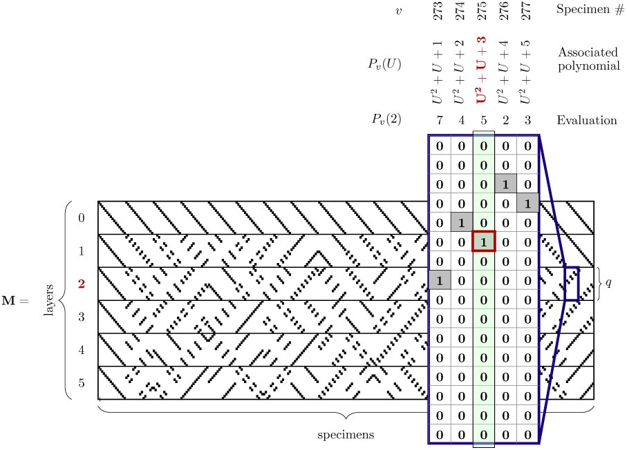 Fig. 1
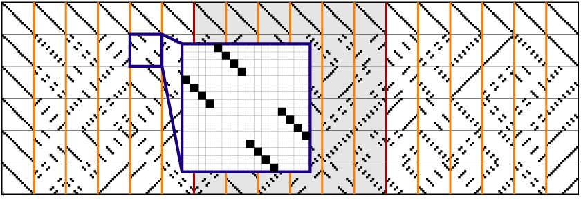 Fig. 2
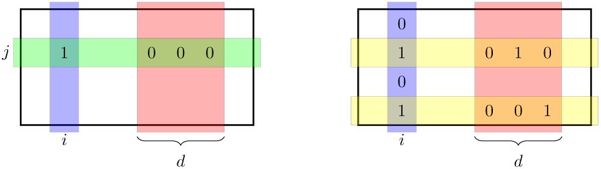 Fig. 3
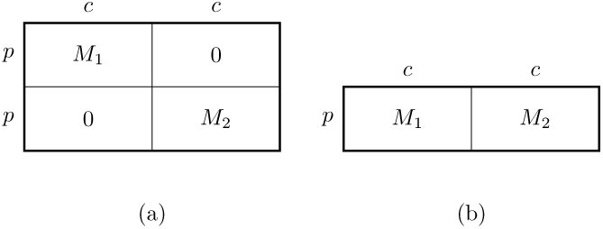 Fig. 4
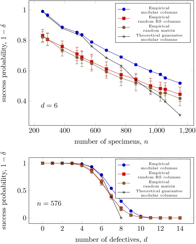 Fig. 5
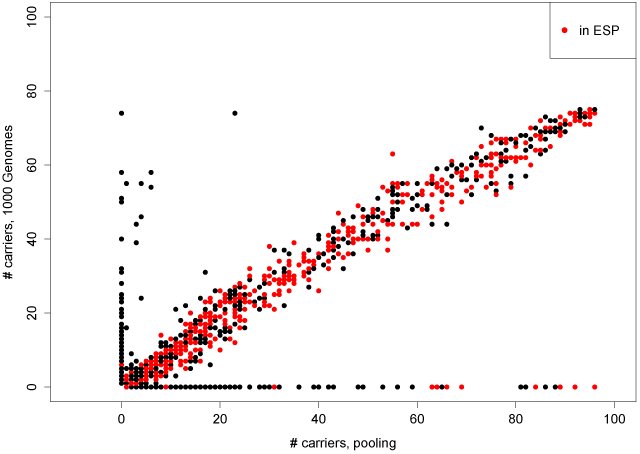 Fig. 6







Peer Reviews
No public reviews on file for this paper yet. If you reviewed it on a platform where reviews are public (OpenReview, ICLR, NeurIPS, ICML), you can paste yours below so the community can read it here.
Videos
No videos yet. Explain this paper in a talk, walkthrough, or lecture? Add one.
Taxonomy
TopicsAlgorithms and Data Compression · DNA and Biological Computing · RNA and protein synthesis mechanisms
Significance
We provide a mathematical formulation of biologically relevant structures in combinatorial pooling designs. Before this work, biologists had not articulated in precise ways the type of structures necessary or useful in pooling designs. We also show that Reed-Solomon codes, and more generally linear codes, satisfy all of these mathematical properties. We establish fresh connections between biologically relevant and combinatorial properties of error correcting codes and how to construct practical, relevant pooling designs with rigorous guarantees.
Introduction
The field of molecular biology increasingly relies on large screens where overwhelming numbers of specimens are systematically assayed in the search for a particular outcome. These screens can come in various forms: systematic testing of tens of thousands of small molecules in a search for potential drugs; interfering with the activity of every gene in the genome to elucidate the organization of genetic networks that underly cancerous processes using RNAi; determining the ability of one protein to bind to every other protein in the genome in yeast two-hybrid systems; and testing the association between virtually every possible genetic variation in the genome and some phenotype of interest such as diabetes or heart diseases. One advantage of these screens is that they are considered “hypothesis-free,” letting the data reveal new and unexpected outcomes that are hard to deduce from current biological knowledge. The downside is that screens can be quite resource and energy consuming. In many cases, screens “waste” an overwhelming number of assays that deliver negative and uninteresting results to find the scarce positive findings.
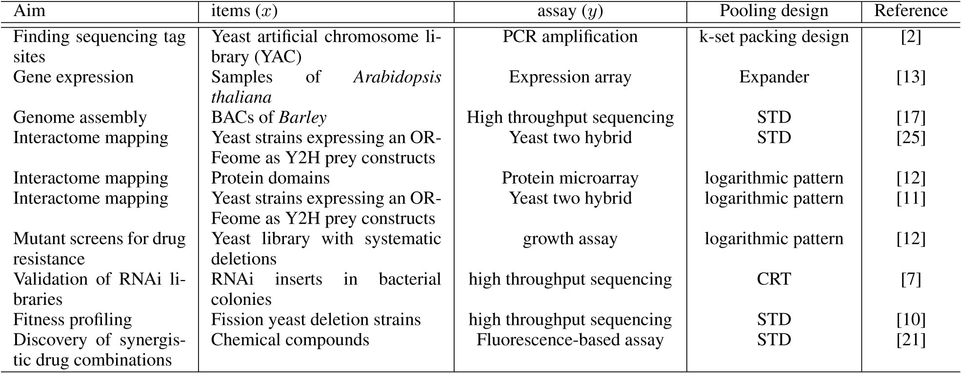
In the last few years, we and others have independently demonstrated screens in various biological domains that are based on combinatorial pooling (see the Table in the supplementary material). These experiments have two basic commonalities. First, instead of independently assaying each one of the specimens, the experiments begin with grouping the specimens into pools using specific mathematical rules, and then assaying the pools. This procedure dramatically reduces the costs of the experiments as the number of pools is much smaller than the number of the original specimens. Second, in contrast with naive pooling in which a group of specimens participate in exactly one pool, each specimen in combinatorial pooling participates in a series of unique pools. Thus, it is possible to assign a unique result to each specimen by comparing the pattern of the results to the pooling design, as long as the number of positive findings is relatively small.
Most of the experiments above exploited non-adaptive group testing or compressed sensing to design the pooling pattern. These two closely related mathematical domains deal with construction of efficient designs that reduce the number of pools while preserving the ability to assign unique results to each item. Under these frameworks, biological screens are cast as a system of (linear) equations [eqn] with n variables, each variable corresponds to an item in the screen. The items can come in different forms: small molecules in chemical screens, different hairpins in RNAi screens, a library of preys in yeast two-hybrid screens, or human individuals in genetic studies. The aim of the screen is to uncover x, a vector of length n, whose ith position denotes the biological property of item i. For example, in a small molecule screen, x can be either 1 or 0, where 1 denotes an active compound and 0 denotes an inactive compound. The experimenter does not observe x directly. Rather, she employs t assays into which the n items have been pooled and observes y, a vector of length t whose jth position denotes the assay results for jth assay. For example, in a small molecule screen, the entries of y can denote the fraction of surviving cells in the presence of the compound, or y can be a vector with entries that are either 0 or 1, where 0 means that no cell survives while 1 captures the survival of some of the cells in the assay. Finally, we can express the pooling design by M, a matrix with t rows and n columns whose entries are non-negative numbers. The entry M_ij_ = r means that r-units (micrograms, microliters, moles, or some arbitrary measure) of item j are assayed in the ith reaction. With this representation, trivial screens (no pooling) simply correspond to the n × n identity matrix; each items is assayed in exactly one distinct reaction. The noise ϵ can be zero, a random variable, or an arbitrary, bounded value, depending on the model. In group testing, the product Mx is computed using Boolean arithmetic: the result of an assay is positive if and only if at least one sample in the pool is positive. In compressed sensing, the entries of the matrix M are real numbers and the product Mx is computed using standard real-valued arithmetic.
Unfortunately, the theoretical work in group testing and compressed sensing does not address many practical design challenges biologists face in using such pooling strategies. Significant progress has been made in developing pooling designs with a minimal number of assays but with scant attention to whether these designs can be implemented in practice.
Here, we map the current implementation gaps and propose a mathematical framework based on coding theory that addresses most of these barriers. We also describe experimental validations of Reed-Solomon code and provide an overview of web-based tools that we have developed for creating and implementing pooling designs at the bench. Using these tools, experimentalists with no mathematical knowledge in coding theory and minimal equipment can conduct complex pooling experiments.
Challenges and Results
Features of practical pooling designs. In the last few years, we have conducted dozens of large scale pooled screens in various biological domains that highlight common features and issues in implementing pooled experiments.
Well-balanced designs. We noticed that the most implementation-robust designs are well-balanced designs, where each item is pooled exactly the same number of times and all the assays have (close to) an identical number of items. These designs consume the same amount of material from all items, allowing straight forward planning of the experiment and reducing the risk that an item will run out during pooling. It also ensures that each item is treated equally. Assays with identical numbers of items are also highly beneficial. They produce more consistent results that mitigate the effect of diluting the specimens. Another by-product is that well-balanced designs allow fast quality assessment of the pooling procedure before starting the expensive screening step. Large deviations in pool volumes or in the residual specimen material can be easily detected by eye and serve as an indicator that there was a potential flaw in constructing the pools.
Maximal utilization of biological kits. A large number of biological kits are sold in batches of 96 assays to fit the common microtiter plates. In many realistic scenarios there are minimal cost differences between a design with 50 assays or 96 assays, but a significant difference between a design with 96 pools and 97 pools. Thus, it is desirable to find a pooling design with a multiple of 96 assays. Of course, one can construct a random pooling design to achieve this aim, but then the design will not be well-balanced. Thierry-Mieg [22] proposed the Shifted Transversal Design (STD), which is a well-balanced and was widely used in biological experiments. Unfortunately, STD cannot fully utilize a 96 well plate, as it produces numbers of pools that are a small multiple of a prime number (smaller than the prime itself).
Light Weight. Most theoretical pooling designs do not take into account the weight of the design, that is, the number of 1s in M. The weight is a critical feature for pooled experiments. Heavy weight means that each specimen is sampled more times, which consumes more material. In theory, of course, we can take a smaller amount of each specimen to mitigate this problem. But in reality, conventional liquid handling robots cannot accurately aspirate and dispense small quantities, limiting the possible weight. In addition, heavy weight designs are more laborious to implement and have higher overheads, contributing to the costs of the pooling procedure (robotic time, tips, or manual labor). In our experience and survey of the literature, tractable pooling designs rarely exceed a column weight of 10 in many cases.
Modularity. When the number of input specimens is large, a pooling experiment is typically divided into batches of distinct blocks of specimens. For each batch, the experimentalist essentially starts from scratch to construct the pools with the new subset of specimens. This approach is more robust because a sporadic failure of the liquid handling system affects only a limited number of specimens rather than the entire experiment. In addition, it limits the amount of liquid evaporation from the pools by minimizing the time it takes to finish constructing a pool. One desired property is that every batch will have a good performance and that the experimentalist will be able pool distinct batches together into a ‘mega-design’ without too much loss of performance. This will allow maximal flexibility in carrying out the multiple experiments. For instance, the experimenter can start with a conservative pilot experiment on one batch. Based on the results, she can decide whether to take a more aggressive approach and pool multiple batches together into a mega design or to retain the more conservative approach. Another advantage of modular designs stems from the fact that the constructed pools will typically be used many times in various conditions (e.g., using different bait proteins in yeast two-hybrid experiments), with varying numbers of positive items. A mega design can be sufficient in most cases, but decoding may fail when the number of positives is unusually high. However, when this happens one can redo the experiment using the underlying sub-designs, which have more smaller pools and will thus successfully identify the positives.
Average performance. Substantial parts of the theory of group testing address the worst-case performance of a pooling design, called the matrix disjunctness. With this property, it is very easy to derive the minimal number of positive items that can be decoded after pooling given a certain number of errors. In practice, however, the worst-case performance has low utility for experimentalists. What we really need is a design that performs well on average and to know the expected rather than worst case performance of the design.
Robustness to Noise. Much of classical group testing theory deals with the case of perfect measurements; i.e., we observe y = Mx. In practice, almost all measurements performed by experimentalists are noisy. We therefore need pooling designs and reconstruction algorithms which provide good average performance in a noisy setting. Up to now, these last two points have only been adressed by simulation [23].
Reed-Solomon based pooling designs. We have found a pooling design based on Reed-Solomon (RS) error correcting codes that dramatically reduces the number of pools compared to the pooling designs widely used in biological experiments, while addressing the practical properties mentioned above. In coding theory, a code is a set of vectors that differ pairwise in a large number of places. RS codes are linear codes, based on polynomials over finite fields.
Designs based on RS codes have been used in biological group testing since the 1960’s, when they were proposed by Kautz and Singleton [14]. However, existing work has not addressed the challenges above; the contribution of this work is showing how to use RS designs to address the practical needs of modern biology.
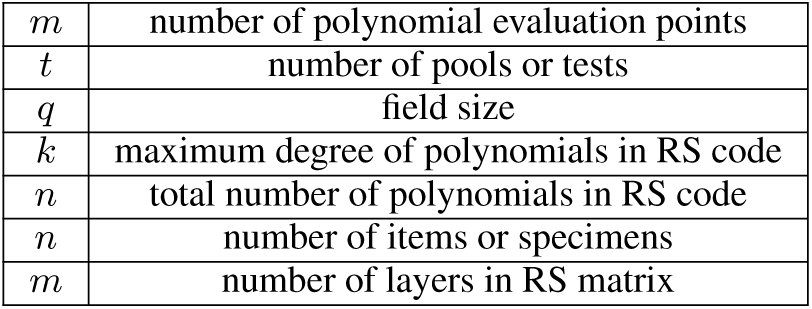
Below, we describe the construction of a RS design from the practitioner’s perspective; the supplementary material contains a more theoretical approach. We build the matrix M by stacking smaller submatrices, called layers on top of each other. The basic construction starts by selecting three integers: q, the number of pools in each layer, m, the number of layers, and k, the maximum degree of the polynomials we construct. We refer to such codes as [m, k, m − k + 1]q-RS codes. There are three constraints on these parameters, imposed by the theory. First, the number of specimens, n, must be at most q_k_; in practice, we will choose k to be the smallest integer so that this is true. Second, q must be either a prime or a prime power (e.g., 7, or 2^4^ = 16). For practical reasons discussed later, we are interested specifically in the case when q = 16. Third, both k and m must be smaller or equal to q. The pooling matrix M has t = qm rows (pools), and is divided into m submatrices (layers) of equal size q × n. We will number the layers 0, 1,…, m − 1, and we will number the rows within each layer 0, 1,…, q − 1.
Next, we represent each specimen number as a polynomial of degree k−1. We order the polynomials lexicographically. For example, if k = 3, and q = 16, then the first specimen is represented by the polynomial P0(U) = 0U^2^ + 0U + 0 = 0, the second specimen is represented by the polynomial P1(U) = 0U^2^ + 0U + 1 = 1, the 275th specimen is represented by P275(U) = U^2^ + U + 3, and the 276th by P276(U) = U^2^ + U + 4. Notice that this polynomial representation depends on q: if q = 7, then P275(U)=5U^2^ + 4U +2.
Each specimen will be assigned to one pool in each layer. To find the pooling assignment of the ith specimen in the jth layer, we will evaluate the polynomial P_i_ at position j, P_i_(j), over the finite field of size q, denoted [eqn]. For example, if q = 7, i = 275, and j = 2, then P275(2) = 5 · 2^2^ + 4 · 2 + 3 mod 7 = 3.
Now, the i column in the j layer is a binary vector of length q, whose ℓ-th position is 1 if P_i_(j)= ℓ and 0 otherwise. Thus the ith sample will be assigned to the ℓth pool in the jth layer. For example, if q = 7, in layer 2, the 275th specimen will be assigned to the pool labeled 3 in that layer.
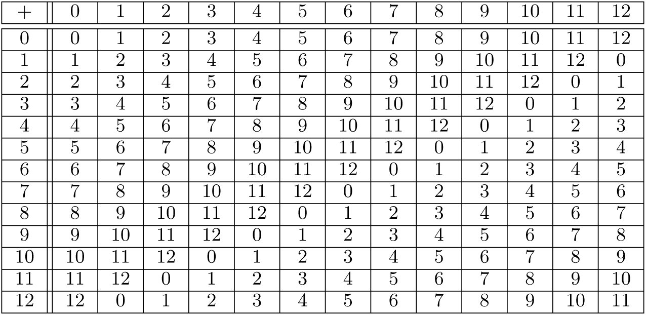
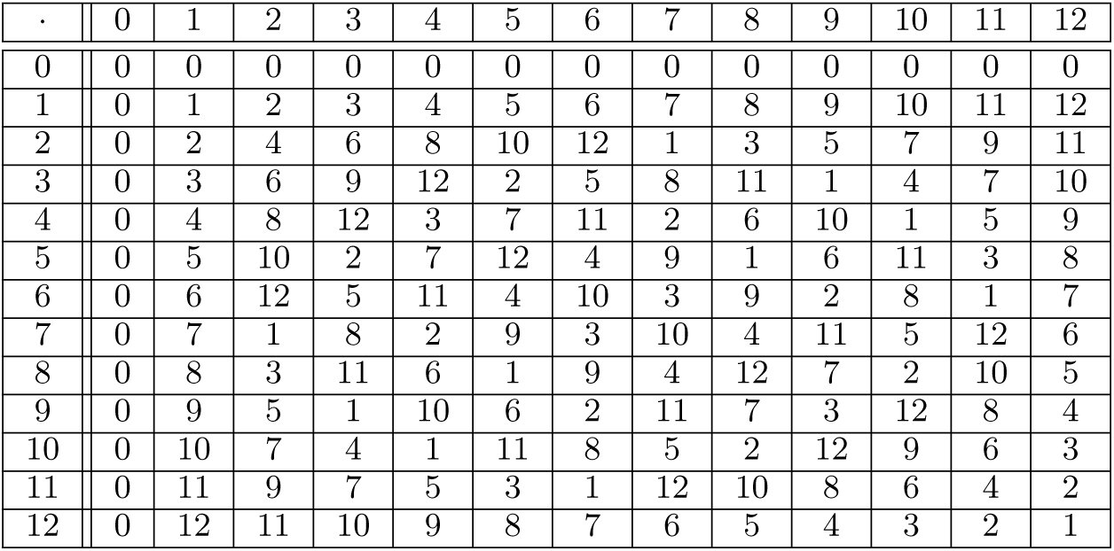
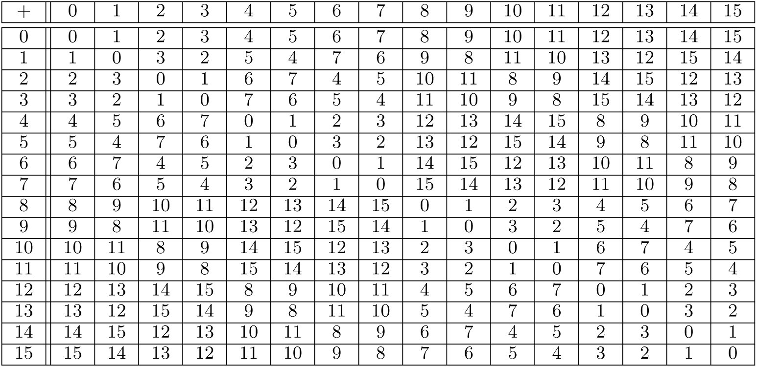
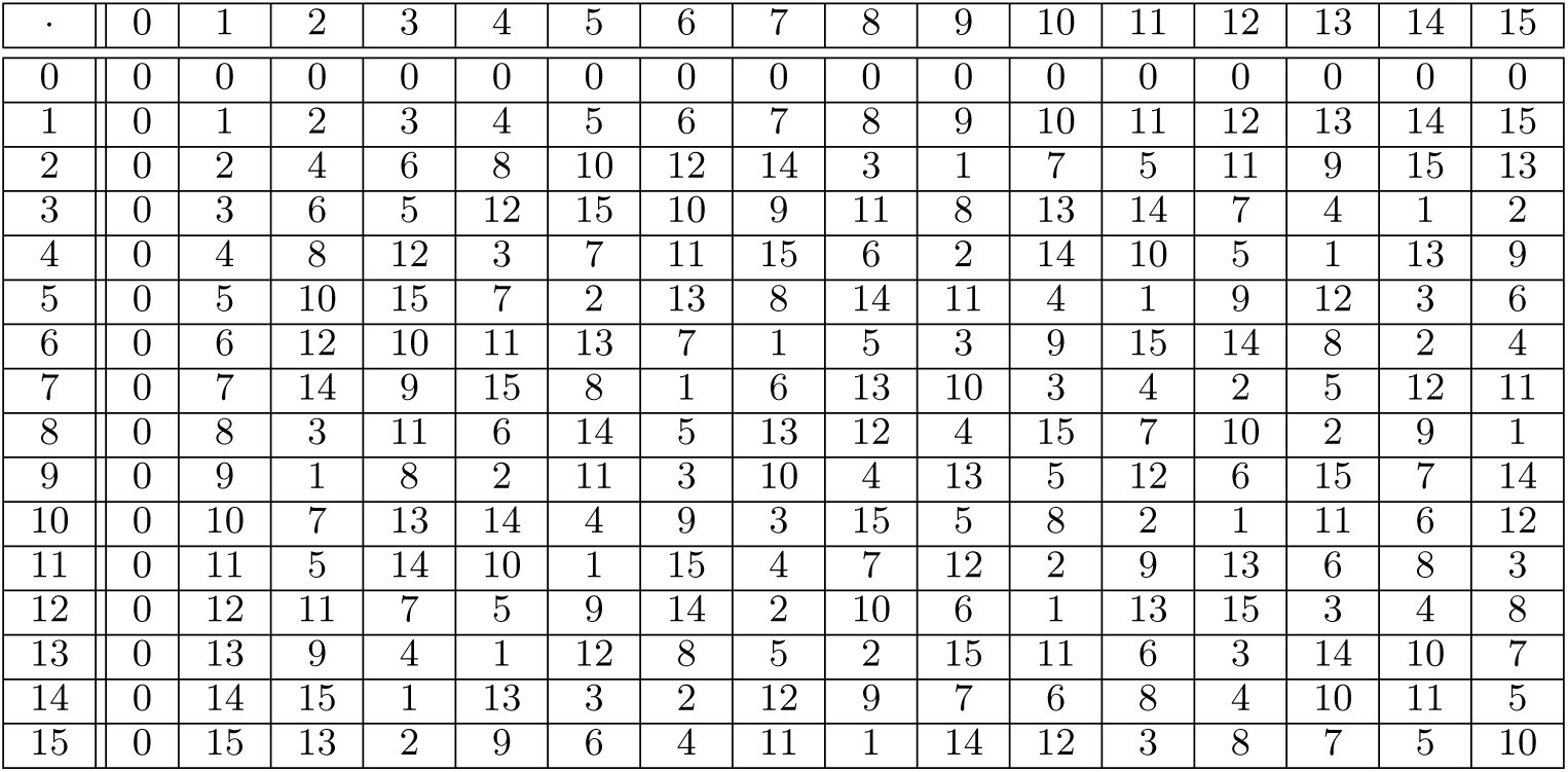
We note that when q is a prime number, the addition and multiplication operations to evaluate the polynomial are simply performed modulo q. However, when q is a prime power, the arithmetic of the finite field is more involved—for example, over [eqn], we have 4^2^ = 3. We have included in the supplementary material an introduction to finite fields and arithmetic tables for [eqn]. In this example, if q = 16, then we consider P275(2) = 2^2^ + 2 + 3 over [eqn], which turns out to be 5. Thus, the 275th specimen will be assigned to pool 5 in layer 2.
The process is illustrated in Figure 1, with q = 16, m = 6, and n = 288. We will return to this example throughout the paper to illustrate our ideas.
Construction of the Reed-Solomon pooling matrix with q = 16 and m =6, and n = 288. The columns corresponds to specimens and are indexed by polynomials over , and the rows are grouped into 6 layers. We highlight the assignment of the specimen v = 275 in layer 2. As described in the text, we consider P275 = U2 + U +3, and evaluate P275(2) = 5.
Returning to the example of Figure 1, we see that the resulting design matrix is balanced. In each 16 × 16 block, there is exactly one 1 in each row and each column. This implies that (a) each of the 288 specimens participates in exactly 6 pools, and (b) each pool contains exactly 288/16 = 18 specimens. Further, it implies that these properties hold modularly: the design given by the shaded submatrix has 96 specimens, each of which participates in exactly 6 pools, so that each pool contains exactly 6 of these specimens.
Shifted Transversal Designs [22] are special cases of RS codes, when q is limited to a prime rather than a prime power. We describe the correspondence in the supplementary material. We will show that RS codes possess all the qualities of STD, while providing more flexibility: contrary to STD, RS codes are instrinsically well–adapted to typical laboratory automation hardware.
Structural Properties of Reed Solomon pooling designs
From the constructions of RS designs, we immediately see that several of our practical desires are met.
First, the parameter space is very rich, and in particular this allows for designs which fully utilize 96-well plates. As in the example above, choosing m = 6 and q = 16 yields precisely 96 wells. Further, as the specimens are also stored in 96-well plates, it is convenient for pooling designs to work with n specimens, where n is a multiple of 96. Again, the example above (where n = 288 = 3 · 96) demonstrates that this is easily obtainable. Further (as can be seen in Figure 1), these designs have a lot of structure, resulting in more efficient pooling as well as error checking of the pooling procedure by visual inspection.
Second, these designs enjoy excellent regularity and weight. Each specimen is pooled into exactly one pool in each layer; thus, each specimen participates in m pools total. It is also true that each pool contains exactly n/q specimens, as long as n is a multiple of q.
This fact implies very strong regularity properties: not only are the designs light and well-balanced, but these properties hold in a modular fashion. As described above, it is often useful to be able to pool different sets of specimens at different times. With RS designs, as long as the specimens are pooled in multiples of q, the scientist enjoys light and well-balanced designs in whatever sizes are convenient.
Disjunctness and recovery. In addition to convenient structure, the pooling design should allow for efficient recovery of the pattern of positive specimens, given the pooled data. For this, we introduce the notion of disjunctness. A pooling design is d-disjunct if for every set Λ of d specimens, and every specimen i not in that set, there is some pool j that includes i but doesn’t include any item in Λ. The resulting condition on the matrix M is illustrated in Figure 3. If M has this property, then we can quickly find the correct set of positives from the pooled results, assuming this set is not larger than d. We simply assert that an item i is positive if all of its pools were positive. If the item i was not positive, and the true set of positives was Λ, then the disjunctness condition precisely states that i will land in some pool that does not test positive. Disjunctness is discussed in more detail in the supplementary material.
A pooling design is d-disjunct if for all Λ of size d and all i, there is a row j as in the lefthand diagram. In contrast, the matrix on the right is not d-disjunct.
For pooling designs arising from codes, like RS designs, it is easy to obtain a bound on disjunctness. The RS design defined above has disjunctness at least d = ⎿(m − 1)/k⏌. In our running example from Figure 1, this comes out to d =2. We will see in a later section (Proposition 2) why this is the case. In terms of the number of specimens n, the above bound guarantees that with t pools we can achieve disjunctness of a least [eqn]. This bound gives a trade-off between recovery guarantees (the maximum number of defectives recovered, d) and budget (assumed to be proportional to the number of pools t). Moreover, the RS-based design described above is incremental - that is, an experimentalist can start with a small number of layers m, giving a small pooling matrix M with a certain disjunctness value, and gradually increase m by adding additional layers to the pooling matrix, hence increasing the disjuncness. Adding an additional layer j is easily achieved by evaluating the polynomials p_i_ over the field [eqn] at the element [eqn].
Modularity
As discussed in the introduction, in many applications it is convenient to pool samples in batches, so that these batches may either be tested independently, or mixed with others and tested jointly. More specifically, given two groups of c specimens each, one may pool each group separately (using two different pooling designs) into p pools each; the resulting design has 2c specimens pooled into 2p pools. Alternatively, one may combine or “superpose” the designs, resulting in 2c specimens pooled into p pools. The resulting situation for measurement matrices is shown in Figure 4.
Different ways of combining two pooling designs given by matrices M1 and M2. In (a), each group of specimens is pooled separately, resulting in 2p pools. In (b), the pooling designs are combined, resulting in p pools. A design M consisting of submatrices M1,M2 has good modularity if the pooling matrix (a) has strictly better disjunctness than the matrix (b).
There are trade-offs between these two strategies: in the first, there are more tests but there are fewer specimens in each pool, potentially yielding more accurate assay results. In the second, there are fewer tests, but a possibility of less accuracy. One practical goal in pooling designs is to make this trade-off as beneficial as possible. That is, we would like to partition the columns of the pooling matrix M into submatrices M_i_ so that each submatrix M_i_ has good disjunctness. Trivially, each M_i_ will be at least as disjunct as M itself, but we seek designs where passing to a submatrix yields a strict improvement in disjunctness (and hence a strictly better trade-off between the accuracy and the number of pools). We refer to this property as the modularity of the design, and we discuss the mathematical particulars in more detail in the section on general linear codes.
Even without improving disjunctness, the smaller designs corresponding to submatrices M_i_ are easier to decode because the d positives will be spread across these subdesigns, so that each experiment will have to deal with (and identify) fewer positives.
In practice, there are many reasons that one might wish to have the kind of flexibility that modularity entails. For example, suppose—as is often the case—that one does not know the true number of positives, d. Then one may use modularity to estimate d on the fly, as follows. Suppose that the pooling design is given by a modular matrix M, which decomposes into submatrices M1,M2,…,M_b_, where each submatrix M_i_ assigns, say, 96 items to p pools. Before doing any tests, the biologist may pool her samples into b different 96-well plates, according to the b different pooling designs, each with very good disjunctness. When it is time to run tests, she may choose to start with a single plate; if her results are very good, she may think that she has over-estimated d. For her next two tests, she may choose to combine the second and third plates, which results in a design (as in Figure 4(b)), with worse disjunctness but fewer pools. If this still appears too pessimistic, she may continue in this way, testing more and more plates at a time until she hits the desired trade-off between disjunctness and the number of pools.
As another example, the Shifted Transversal Design has good modularity, and this has provided important practical benefits in an interactome mapping experiment [25]. In this work, subdesigns (“micro-pools”) were constructed once, and were then combined by superposition to obtain designs that were well–suited to various experimental formats: in pairs for the 1536–well format, in sixes for the 384–well format, and in twelves for the 96–well format.
RS designs (and, as is the trend in this work, designs from appropriate linear codes more generally) have good modularity properties. The basic idea is that each slab of q columns (demarcated by the orange lines in Figure 2) has similar disjunctness properties. This follows from the fact that the sets of polynomials they correspond to look similar: as far as disjunctness is concerned, there is not much difference between the set {U^2^ + U, U^2^ + U +1,…,U^2^ + U + 15}and the set of constant polynomials {0, 1,…, 15}. Similarly, at a larger scale, there is not that much difference between the set of all polynomials of the form U^2^ + aU + b and the set of all polynomials of the form 2U^2^ + aU + b.
Because of the nature of these symmetries, the modularity naturally occurs for sets of columns of size q, q^2^, q^3^, and so on. For example, when q = 16, m =6, and k = 3, we may support up to n = q^k^ = 16^3^ = 4096 items with disjunctness 2. These items can be divided into subsets of size 16^2^ = 256 with a guarantee of disjunctess 5. However, as discussed above, it is often convenient if the sizes of the subsets of specimens are multiples of 96. For illustration purposes, consider a slightly larger version of our running example, where q, m, and k are as above, but where n = 576 =6 · 96. If we split up the specimens into six batches of size 96 in the natural way: the first 96 columns, then the next 96 and so on, most of the blocks of size 96 do not interfere with the blocks of size 256 (or do not overlap the 256-block boundaries). Thus, most batches of 96 specimens obtained this way inherit the improved disjunctness of the blocks of size 256. This same argument works for any multiple of 96.
Average disjunctness
Whether we exploit the modularity of the RS design or not, the entire design of our running example has disjunctness of only two which seems rather bleak. Unfortunately, with only 96 pools and a large number of samples, it is not possible to obtain much better worst-case guarantees. However, in practice, these guarantees are often overly pessimistic. Thus, it is natural to ask about the performance of these designs against most patterns of positives. We seek a statement of the form, “for most patterns of defectives, the group testing matrix is effectively d-disjunct.”
To this end, we define a weaker notion of disjunctness, which we call the average disjunctness, which measures how many defectives can be reliably identified in a “typical” rather than worst-case situation. We say that a set Λ of specimens is bad if it causes a situation as in the right-hand side of Figure 3. That is, Λ is bad if there is some specimen i so that i coincides with at least one member of Λ each time it is pooled. Thus, a design is d-disjunct if all sets Λ of size d are not bad. We relax this in a natural way, and say that a pooling design is (δ, d)-average-disjunct, if at most a δ-fraction of the sets of specimens Λ of size d are bad. (When δ is not mentioned, we take it to be an appropriate small constant, like 0.01).
Thus, if the positive specimens are randomly distributed, with probability 1−δ, the set of positive specimens that appears is not bad. Thus, by the same reasoning about the (worst-case) disjunctness, we conclude that (δ, d)-average-disjunctness allows efficient identification of d positives chosen uniformly at random with probability at least 1 − δ. Of course, it is unreasonable to assume in practice that the positive specimens will be uniformly distributed. However, the above reasoning works for any distribution which is “close” to the uniform one in an appropriate sense; e.g., physical specimens are assigned column identities at random.
A matrix may be d-average-disjunct without being d-disjunct, and we are interested in quantifying and exploiting this gap. We do so both in practice and in theory. In the supplementary material, we show how to efficiently compute simple, provable bounds on the values of (δ, d) so that RS designs are (δ, d)-average disjunct. We complement our theoretical results with empirical ones, which indicate that our bounds are quite accurate for small d, and lose accuracy as d grows.
Our results, both theoretical and empirical, are displayed in Figure 5. We compared the empirical performance of the RS pooling design to two randomized designs. For the first random design, we chose n random columns from an RS design with the full q^k^ possible columns; this comparison is meant to illustrate that our modular column selection is not only convenient for practical considerations, it also actually yields better performance. For the second random design, we chose a random m · q × n matrix with m ones per column. Theoretically, random matrices offer the best asymptotic guarantees, and so the fact that RS designs outperform it for reasonably sized values of n is striking.
Empirical and theoretical bounds on (δ, d)-average disjunctness for RS designs. In both charts, the empirical performance of the RS pooling design is compared to its theoretical performance, as well as the empirical performance of two randomized pooling designs. For the RS matrices, empirical performance was judged using 5000 random trials. For the random matrices, empirical performance was judged from 100 trials each on 100 random matrices. The theoretical bounds were obtained through a recursive formula described in the supplementary material. The top chart traces the empirical and provable success probability 1 − δ of a RS design with m = 6 and d = 6, as the number of specimens n grows, and compares this to the failure probability of random designs with the same column weight and number of tests. The bottom chart fixes n = 576 = 6 · 96, and varies d. For all RS designs, the worst-case disjunctness is two.
These results are much more hopeful than the worst-case bounds of d = 2. For n = 576, for example, up to 7 or 8 positives may be accurately identified with reasonable probability. Further, we see that RS designs perform much better than comparable randomly generated designs.
Experimental validation of RS-based pooling
We tested the RS design with an experiment that combined 480 samples into 96 pools (m =6, q = 16). For this experiment, we used a toy problem in which individual samples were represented by a single well of 150 µ1 of deionized water and positive samples of water were spiked with blue dye (100X dilution). The aim of the experiment was to find the positive (blue dye) specimens by inspecting the pools. Pooling was carried out with a Tecan Evo robot using a four-tip liquid-handling arm (LiHa). To acquire the data, we quantified the absorbance ratio (470nm/630nm) of each pool using a plate reader. Then, we used an out-of-the-box conventional compressed sensing decoder (GPSR) [19] to decode the results.
Despite the molecular simplicity, our experimental design captures some of the challenges inherent to pooling experiments. First, it tests the actual execution in a laboratory setting. Second, this simple experiment captures the three main challenges of pooling experiments: pipetting, dilution, and measurement noise. Pipetting noise refers to the inability of the experimentalist to aspirate and dispense the exact volume of the input specimen due to human error. These imperfections introduce noise to the pooling matrix that can distort the signal. Based on our empirical results, the coefficient of variation of the pipetting steps was 5–10%. Dilution noise occurs when the signal from the positive specimen is diminished as the size of the pool increases. In our toy experiment, each pool contained 30 specimens, diluting the blue dye signal by the same factor. Measurement noise in this example would result from the absorbance scan to measure the blue dye of the constructed pools. In this case, the measurement noise mainly originated from the number of photons of each scanned pool.
Despite these imperfections, we were able to accurately decode the pooled results and identify the original specimens when three were positive. We repeated this experiment with ten positive specimens and were able to correctly decode eight of the original specimens with one false positive and one false negative. This is not surprising as simulations shown in Figure 5 exhibit imperfect decoding for similar conditions.
Encouraged by these results, we also tested our pooling design to find rare genetic variations using targeted high throughput DNA sequencing. Targeted sequencing is a labor intensive and costly procedure that processes DNA in multiple steps to enrich for specific genomic regions; instead, we used a pooling design. We pooled equimolar amounts of 96 DNA samples from the HapMap Project into 25 pools using an RS code with m =5 and q =5 (also a Shifted Transversal Design). The 25 pools were barcoded and enriched by hybrid selection using Agilent SureSelect baits that enriched for genes found in the Framingham Heart Study (≈ 790 kb of genomic material). The pools were further compressed into five mega pools and sequenced on five lanes on the Illumina HiSeq (2 × 80 bp) to 1000 times the average coverage per pool.
To test our approach, we examined 75 of our samples that were also sequenced as part of the 1000 Genomes Project [4]. More than 97% of the target region was covered by at least one sequencing read. After filtering positions with low quality data (see supplementary material), we were left with 92% of the bases in the original design. Next, we exploited the structure of the RS code to estimate the number of carriers in our design before decoding and attributing the mutation to individual specimens. This procedure relies on the observation that each specimen participates in exactly one pool per layer. By inspecting the number of variant reads across pools in the same layer, it is possible to estimate the number of carriers. Since our design had five layers, we repeated this procedure five times and averaged the results to get more accurate estimates. We compared the number of carriers between our estimator using the pooling data and an estimator using the individual-level results of the 75 specimens in the 1000 Genomes data. Figure 6 shows excellent consistency (R^2^ = 0.91) between the two estimators (perfect consistency cannot be observed since we have individual level data for only 75 out of 96 samples).
Comparison of carrier rates from 75 HapMap samples between 1000 Genomes and our pooled samples. Further comparison to the Exome Sequencing Project (variable sites are red) suggests that misdetections in our pooled samples are false positives in 1000 Genomes.
Our results also found good decoding capabilities for rare variants. We decoded the pooled data for variants where our pooled estimator indicated five or fewer carriers (translating to a minor allele frequency of 2%). We used a series of decoders that took into account the sequencing noise at each position and the distribution of reads with the variant allele. These decoders ran on each nucleotide separately and used the pooling matrix to find which specimens actually carry the rare allele. Our results indicate a specificity of > 99.99% and sensitivity of about 85% compared to the 1000 Genomes data, averaged across all positions. We wondered if the false negatives represent a true decoding miss or a sequencing error in the 1000 Genomes project due to the low coverage of these genomes. We turned to the National Heart, Lung, and Blood Institute (NHLBI) Exome Sequencing Project (ESP) [8], which contains genomic data for more than 5000 individuals. The expectation is that sequencing errors in the 1000 Genomes data will not appear as variable sites in ESP. Indeed, when we inspected missed positions in our results only 26% of them were variable in ESP. We also inspected positions where our decoder did find a rare variant signal in the pooled data. Close to 38% of those positions were also variable in ESP. This suggests that some of the imperfect sensitivity can be attributed to sequencing errors in the reference data rather than a problem with the decoder.
Tools for Experimentalists
We created a free web tool to design and guide experiments (http://pooling.teamerlich.org). A user uploads a sample map spreadsheet and enters the number of specimens and volume constraints. Then, she can select her desired pooling design (for completeness and education purposes, our tool can generate several pooling designs that are described in the group testing literature in addition to the standard RS code design (q = 16, m =6). Based on user input, the tool checks that the specimens have sufficient volume to be pooled and that the pooling plate can hold the accumulated volume from the input material without spillover. Then, the tool generates a design specific matrix and pooling instructions.
The pooling instructions are compatible with a liquid-handling robot or manual hardware such as iPipet [26]. The latter is a semi-automated open-source tool that we developed to convert a regular iPad (and most tablets) into a sample-tracking device. Users simply place the sample plate and pooling plate on the tablet, and iPipet illuminates the wells to be aspirated or dispensed. Based on our tests, a trained experimentalist can complete an RS-code based pooling experiment of ≈ 500 input specimens within a few hours using iPipet. With this tool and the theory outlined in this paper, we hope to reduce the technical barriers for experimentalists to conduct pooled experiments and to provide guidance based on rigorous theoretical analysis.
The reference list from the paper itself. Each links out to its DOI / PubMed record.
- 1Noga Alon and Joel H. Spencer. The probabilistic method. Wiley-Interscience Series in Discrete Mathematics and Optimization. John Wiley & Sons Inc., Hoboken, NJ, third edition, 2008.
- 2W. J. Bruno, E. Knill, D. J. Balding, D. C. Bruce, N. A. Doggett, W. W. Sawhill, R. L. Stallings, C. C. Whittaker, and D. C. Torney Efficient pooling designs for library screening. Genomics, 26(1):21–30, Mar 1995.
- 3K.-M. Cheung. Identities and approximations for the weight distribution of q -ary codes. IEEE Transactions on Information Theory, 36(5):1149–1153, sep 1990.
- 4The 1000 Genomes Project Consortium. A map of human genome variation from population-scale sequencing. Nature, 467(7319):1061–1073, 2010.
- 5Thomas H Cormen, Charles E Leiserson, Ronald L Rivest, and Clifford Stein. Introduction to algorithms. MIT press, 2001.
- 6Koboldt DC, Chen K, Larson DE Wylie T, Mc Lellan MD, Mardis ER, Weinstock GM, Wilson RK, and Ding L. Var Scan: variant detection in massively parallel sequencing of individual and pooled samples. Bioinformatics, 25(17):2283–2295, 2009.
- 7Yaniv Erlich, Kenneth Chang, Assaf Gordon, Roy Ronen, Oron Navon, Michelle Rooks, and Gregory J Hannon. DNA Sudoku—harnessing high-throughput sequencing for multiplexed specimen analysis. Genome Research, 19(7):1243–1253, July 2009.
- 8Exome Variant Server. NHLBI GO Exome Sequencing Project (ESP), Seattle, WA, March 2013. URL: http://evs.gs.washington.edu/EVS/).