An Approximate Markov Model for the Wright-Fisher Diffusion
Anna Ferrer-Admetlla, Christoph Leuenberger, Jeffrey D. Jensen, Daniel Wegmann

TL;DR
This paper introduces a new computational method to infer selection and population size from time series genetic data, improving accuracy in evolutionary studies.
Contribution
A novel discrete approximation for diffusion processes called mean transition time approximation is introduced for joint inference of selection and demography.
Findings
The approximation accurately describes allele trajectories through time with few states.
The Bayesian inference approach accurately infers population size and selection coefficients.
The method identifies selection targets and larger population sizes in Influenza virus evolution data.
Abstract
The joint and accurate inference of selection and demography from genetic data is considered a particularly challenging question in population genetics, since both process may lead to very similar patterns of genetic diversity. However, additional information for disentangling these effects may be obtained by observing changes in allele frequencies over multiple time points. Such data is common in experimental evolution studies, as well as in the comparison of ancient and contemporary samples. Leveraging this information, however, has been computationally challenging, particularly when considering multi-locus data sets. To overcome these issues, we introduce a novel, discrete approximation for diffusion processes, termed mean transition time approximation, which preserves the long-term behavior of the underlying continuous diffusion process. We then derive this approximation for the…
Click any figure to enlarge with its caption.
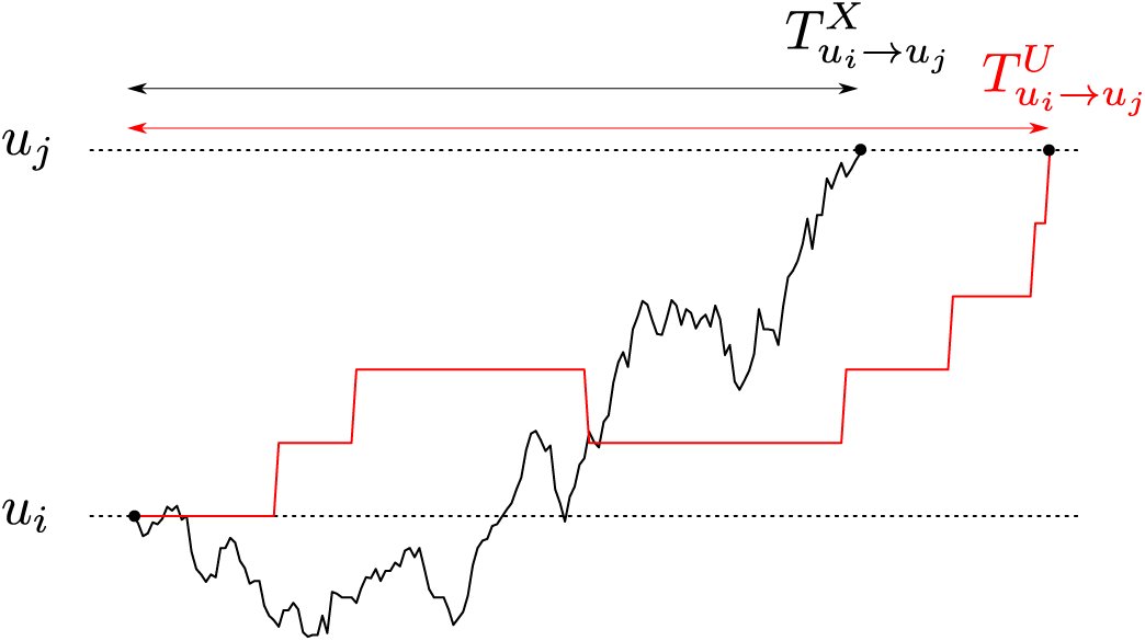 Figure 1
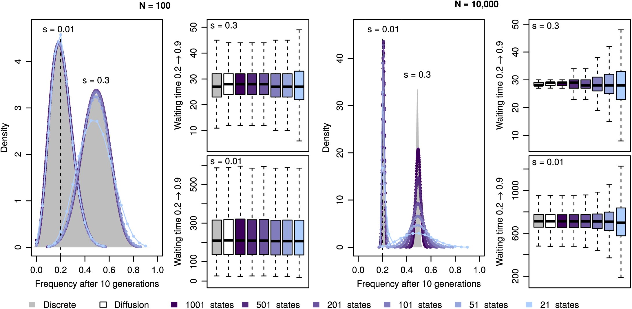 Figure 2
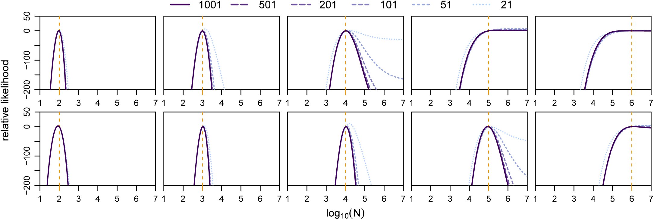 Figure 3
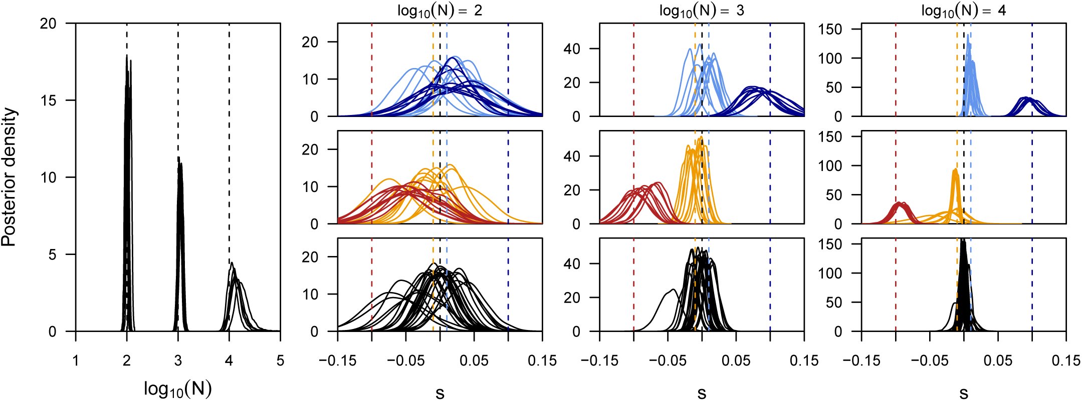 Figure 4
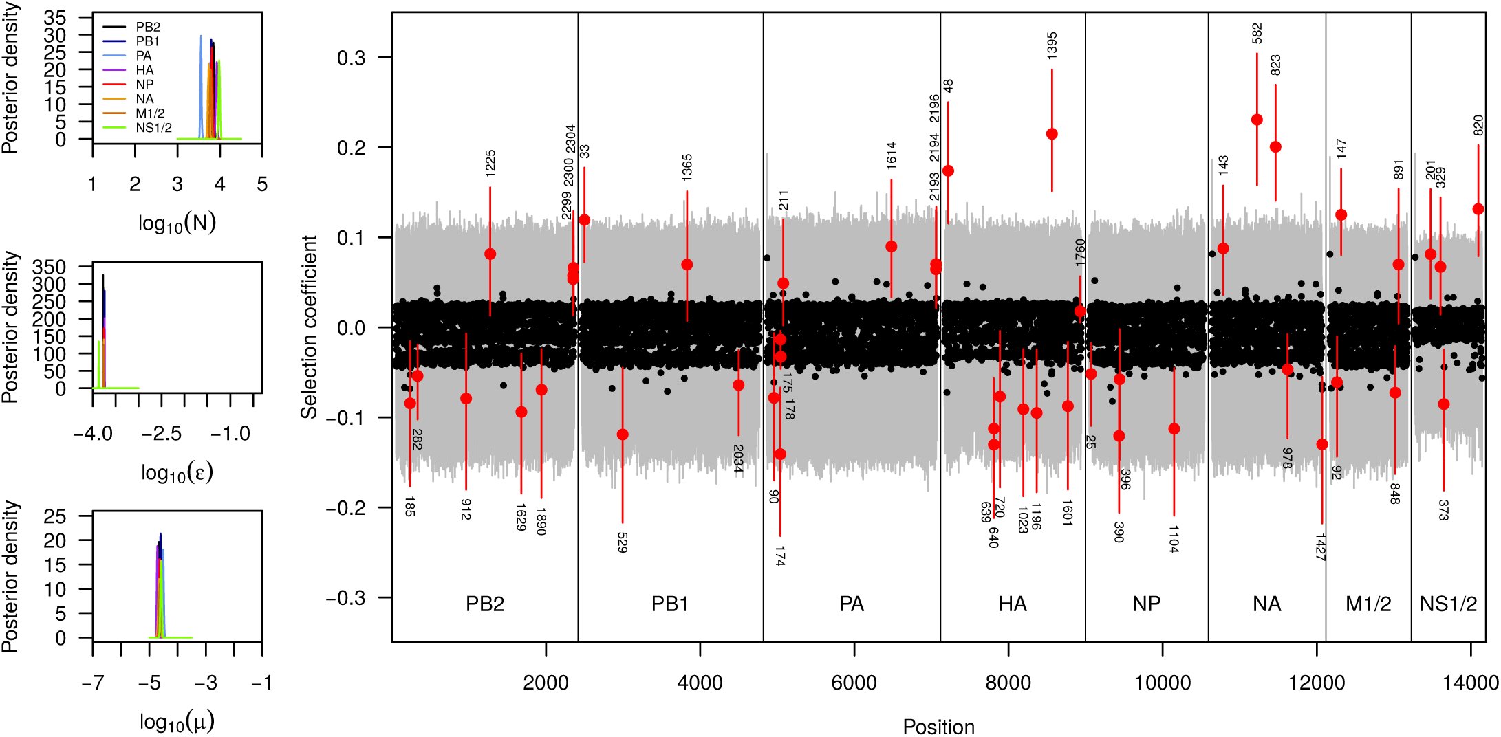 Figure 5


























Peer Reviews
No public reviews on file for this paper yet. If you reviewed it on a platform where reviews are public (OpenReview, ICLR, NeurIPS, ICML), you can paste yours below so the community can read it here.
Videos
No videos yet. Explain this paper in a talk, walkthrough, or lecture? Add one.
Taxonomy
TopicsEvolution and Genetic Dynamics · Mathematical and Theoretical Epidemiology and Ecology Models · Mathematical Biology Tumor Growth
Detecting signatures of past selective events provides insights into the evolutionary history of a species and elucidates the interaction between genotype and phenotype, offering important functional information. Unfortunately, a population’s demographic history is a major confounding factor when inferring past selective events, particularly because demographic events can mimic many of the molecular signatures of selection (Andolfatto and Przeworski 2000; Nielsen 2005). Despite efforts to create statistics robust to demography, all currently available methods to detect selection are prone to mis-inference under non-equilibrium demography.
Some of these issues can potentially be overcome by using multi-time point data, as the trajectory of even a single allele contains valuable information about the underlying selection coefficient. Owing to advances in sequencing technologies, such multi-time point data are becoming increasingly common from experimental evolution (Foll et al. 2014a), from longitudinal medical or ecological studies (Wei et al. 1995; Renzette et al. 2013), and through ancient samples (Wilde et al. 2014; Sverrisdóttir et al. 2014). However, computationally efficient and accurate methods to infer demography and selection jointly from such data sets are still limited.
A natural and common way of modeling such time series data is in a Hidden Markov-Model (HMM) framework, which allows efficient integration over the distribution of unobserved states of the true population frequencies, thus allowing calculation of the likelihood based on the observed samples. Williamson & Slatkin (1999) (Williamson and Slatkin 1999), for instance, developed a maximum-likelihood approach based on such an HMM to infer the population size N from samples taken at different time points. More recently, similar approaches have been developed to infer population size along with the selection coefficient of a selected locus for which time series data is available (Bollback et al. 2008; Malaspinas et al. 2012).
All such approaches, however, are plagued by the problem that the number of hidden frequency states is equal to the population size, which renders HMM applications computationally unfeasible for large populations. Different routes have been taken to overcome this. One approach is to model the underlying Wright-Fisher process as a continuous diffusion process, which is then discretized for numerical integration using a numerical difference scheme (Bollback et al. 2008). Since, this approach remains computationally expensive, it was later suggested to directly model the diffusion process on a more coarse-grained grid (Malaspinas et al. 2012). Under this approach, their generator matrix for the transition between the coarse grained states is then approximated by fitting the first and second infinitesimal moments. Unfortunately, the minimum number of states required is still computationally prohibitive for large values of γ = 2Ns (Malaspinas et al. 2012). For this reason, the most recent reported method resorted to simulation based Approximate Bayesian Computation (ABC), which allowed the joint inference of locus-specific selection coefficients for many loci (Foll et al. 2014a,b). However, this method requires first estimating the population size under the assumption that all loci are neutral, and thus may be biased when many loci are under selection.
Here we introduce a novel framework by approximating the WF-process with a coarse-grained Markov-Model that exactly preserves the expected waiting times for transition between states. This is achieved by exploiting the theory of Green’s function for diffusion processes. Contrary to previous approaches, our approximation matches the WF-process closely even when only very few states are considered, regardless of γ = 2Ns. As we show with extensive simulations and a data application from experimental evolution, our method allows for accurate joint inference of both population size and locus-specific selection coefficients even in the presence of pervasive selection. Further, it is readily extended to incorporate population size changes, sequencing errors or the appearance of novel mutations.
Models
Mean Transition Time Approximation
Let X(t) be a diffusion process on the state space [0,1]. This is a continuous-time Markov process with continuous sample paths and with infinitesimal generator
The classical example in population genetics is the Fisher-Wright diffusion which we discuss below. We seek to find a discrete-state Markov process U(t) which approximates X(t). For this purpose, we subdivide the unit interval [0,1] into, not necessarily equidistant, frequencies
These form the states of U(t). For two states u_i_, u_j_, consider the transition time to first visit of u_j_ when starting at u_i_.
Similarly we define the transition time for the diffusion process X(t). We say that U(t) is a mean transition time approximation of X(t) if [eqn]for all pairs of states u_i_, u_j_ (see Fig. 1). This condition guarantees that the paths of X(t) and U(t) exhibit comparable long-time behavior. In the following we show how to construct the Markov process U(t) from the diffusion process X(t) using the theory of Green’s function.
Mean transition time approximation of Markov processes. Shown are the realizations of a continuous diffusion process X(t) (black) and a discrete-state Markov process U(t) (red) starting at ui until they reach uj for the first time. If the expected waiting time for such a transition is the same for both process for all pairs of states ui, uj, we say that U(t) is a mean transition time approximation of X(t).
We begin by recalling some notions for diffusion processes. The natural scale of the process X(t) is given by [eqn]where [eqn]. The so-called speed measure is defined by
The Green’s function for an interval (u, v) ⊆ [0,1] is given by
Denote by Tx→u or Tx→v the time to first visit of u or v, respectively, starting at x. Then [eqn] is the exit time from the interval (u1, u2), given the process is at x at time t = 0. One can show
Moreover, the probability of exiting at the lower limit u is
We now want to determine the instantaneous transition rates q_i,j_ of the discrete-state Markov process U(t). Recall the definitions [eqn]and
The sojourn time of state u_k_, i.e. the time interval of U(t) spent in state u_k_, is an exponential random variable with parameter q_k,k_. Since the expectation of this exponential variable is 1/qk,k our condition (2) enforces [eqn]where we write k − 1 instead of u_k_ etc. in order to unburden the notation. From this we get [eqn]and
We can now form the tridiagonal generator matrix
The transition matrix of the Markov process U(t) is given by
Application to Wright-Fisher Models
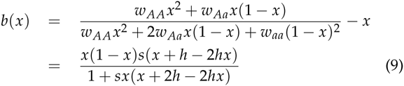
We will consider a classic Wright-Fisher Model of two alleles A and a with fitnesses s and 1 − s, respectively, that segregate in a population of size 2N. Time t is measured in generations of the Wright-Fisher process. In the presence of a non-vanishing dominance coefficient h the fitnesses of the three genotypes are given by w_AA_ = 1 + s, w_Aa_ = 1 + hs, and w_aa_ = 1. Under such a model, the infinitesimal mean, which corresponds to the change in allele frequency, is then given by
Let X(t) be a diffusion process corresponding to the frequency of allele A. An excellent approximation of the Wright-Fisher process is obtained by setting [eqn]and [eqn]in the infinitesimal generator (1), where [eqn]and [eqn]when u_k−_1 ≤ x ≤ u_k+_1
Note that in the standard diffusion approximation the denominator term in b(x) is often omitted. But as shown in (Lacerda and Seoighe 2014), the above choice yields a much more accurate approximation to the WF process.
From (3) and (4) we get [eqn]and [eqn]where we have set
For the speed measure we obtain
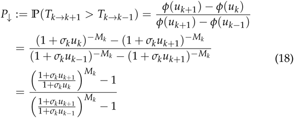
Consider three consecutive states u_k−_1, u_k_ and u_k+_1. For the probability to exit at the lower state we get
The probability for exit at the upper state is
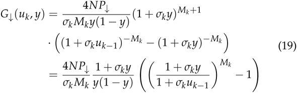
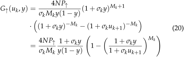
Observe that the Green’s function is calculated by
Using the quantities calculated above we get for the two parts of the Green’s function: [eqn]and
With numerical integration we can determine
Specifically, we use the extended Simpson’s rule for the numerical integration (Press 2007), which we found to give accurate results with typically only 8 or 10 intervals.
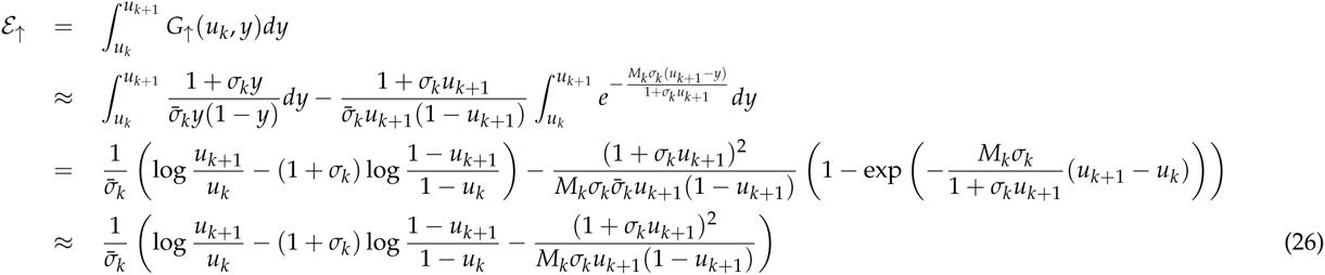
If γ = 2Ns is large, we get approximations for the Green function which allow for analytic expressions of the integrals (see Appendix). Similarly, analytical expressions can be found in the special case s = 0 (see Appendix).
Bayesian Inference
Consider that at the times Tt, t = 0,…, T, samples of sizes M_t_ were taken from the population and m_t_ alleles A were observed in these samples. In this section, we describe how the mean transition time approximation introduced above can be embedded into a Bayesian inference scheme to estimate the population size 2N and the locus-specific selection coefficient jointly from time series data.
As has been noted previously (Williamson and Slatkin 1999; Malaspinas et al. 2012; Mathieson and McVean 2013; Lacerda and Seoighe 2014), a natural way of modeling both the underlying evolutionary process as well as the process of sampling is a Hidden Markov Model (HMM). Under the assumption that the population size between two time points T_t_ and T_t_+1 is constant at N_t_, the transition matrix of such an HMM from state U(T_t_) to state U(T_t_+1) is calculated by [eqn]where Δt = T_t_+1 − T_t_ and the generator matrix Q^t^ is determined as explained above using N = Nt. We note here that this framework allows for instantaneous population size changes to occur at every time t during the HMM. However, we will henceforth only deal with situations in which the population size is assumed to be constant across the whole sampling period.
Following previous implementations (e.g. (Williamson and Slatkin 1999; Malaspinas et al. 2012; Mathieson and McVean 2013; Lacerda and Seoighe 2014)), we will assume that the sampling of alleles from the underlying population frequency is binomial, i.e.
However, for large sample sizes, the few states u_k_ may be too coarse grained to capture the region of high emission probability. We thus propose to integrate the emission probabilities against a smoothing kernel. we chose to implement a beta distribution kernel, which leads to a beta-binomial emission probability that can be evaluated analytically. Specifically, we chose to use a beta-kernel with mean u_k_ and variance [eqn]. Under this choice, the emission probabilities are then calculated by [eqn]where B(·,·) is the Beta function and the parameters α_k_ and β_k_ are determined via the moment estimators for a beta distribution
With both transition and emission probability matrices at hand, we calculate the likelihood of the full data using the standard forward recursion. To be specific, let us first define for t = 0,…, T the (K + 1) × (M_t_ + 1) emission probability matrices
Denoting m1:t = (m1,…, m_t_), we define the total probability
This total probability can be determined efficiently with the forward recursion [eqn]and [eqn]. Then one has [eqn]where we made explicit the dependence of this probability on the parameters [eqn]If we impose priors π(θ) on the parameters then we can simulate the posterior probability π(θ|m1:T) with the usual MCMC scheme using (22) and the Hastings ratio
Extension of basic model
Sequencing errors Generally, sequencing errors are overcome with sufficient coverage. However, in many applications of next generation sequencing to experimental evolution, the goal of the sequencing is not to infer individual genotypes, but rather allele frequencies directly. Under such a setting, each sequencing read is assumed to be from a different individual. In such cases, sequencing errors may lead to false inference, especially when allele frequencies are very small.
Incorporating sequencing errors into our framework is straight forward. Under the assumption that there are only two alleles present at the locus (achieved by, for instance, pooling all non-selected alleles into one class) and symmetric error rates ϵ between those classes, we can approximate the probability that [eqn], the i-th allele survey at time t, is A in the presence of sequencing errors as
Mutational Input We allow for the production of mutant alleles only when the process is in state u0 = 0 or u_K_ = 1. The production of new alleles proceeds at a rate of 2Nµdt. Once a new allele is produced, say when the system is in state u0, it must get from state 1 / 2N into state u1. This happens with probability [eqn] which is calculated according to (7). This yields the transition rate
In the case of positive selection we have
With M = 4N − 1. A similar logic yields
In the selection-free case the transition probabilities are much simpler:
Implementation
We have implemented the proposed model and the Bayesian inference scheme in an easy-to-use C++ program available on our lab website. While we use standard implementations for most aspects, we note the matrix exponentiation in Eq. 8, which is a numerically very demanding problem. A classic algorithm for matrix exponentiation is by diagonalization of the matrix (Moler and Van Loan 1978). While computationally efficient, this algorithm may be numerically unstable for matrices with large conditions numbers, which are typically observed when γ = 2Ns becomes large. This was previously observed by (Malaspinas et al. 2012), who addressed this issue using multiple precision arithmetics. Unfortunately, such arithmetics are computationally very demanding, leading to slow performance of their implementation.
Here, we propose to alleviate this problem using the approximation [eqn]which can be calculated by successive quadration. Such matrix multiplications are generally demanding, but can be implemented in a computationally efficient manner for generator matrices that are tridiagonal, as each quadration step only adds two additional diagonals and such band matrices can be multiplied efficiently (see chapter 7.4 in (Dahlquist and Björk 2008)).
Application to Influenza data
We analyzed allele frequency data from whole genome data sets of Influenza H1N1 obtained in a a recent evolutionary experiment (Foll et al. 2014a). While we refer the reader to the original study for a detailed description of the experimental set-up, we summarize the key point briefly here: Influenza A/Brisbane/59/2007 (H1N1) was serially amplified on Madin-Darby canine kidney (MDCK) cells for 12 passages of 72 hours each to prevent any freeze-thaw cycles. After the three initial cycles, samples were passed either in the absence of drug, or in the presence of increasing concentrations of oseltamivir, a neuraminidase inhibitor for another 9 passages. At the end of each passage, samples were collected for whole genome high throughput population sequencing up to a median coverage of more than 50,000x.
For our analysis here we only considered the time-points taken during drug treatment (passages 4 to 12). As in (Foll et al. 2014a), we excluded all monomorphic sites and those with a coverage lower than 100, resulting in a total of 1427 included sites. For each site, we only kept the two alleles having the highest frequencies over all passages and considered the minor allele to be the one with the lowest frequency at the beginning of the experiment (passage 0). We estimated N along with locus specific selection coefficients s, the sequencing error rate ϵ and the per site mutation rate µ. We assumed log-uniform priors on N, ϵ and µ such that log10(N) U[1,5], log10(ϵ) = U[*−*4, *−0.3] and log10(µ) = U[−*7, *−*1], and a normal prior on the selection coefficients such that s N(0,0.05). Since viruses are haploid, we fixed the dominance coefficient at h = 0.5. We then run an MCMC using 51 states for 25000 iterations during which each parameter was updated in turn. The first 2000 such iterations were discarded as burn-in phase.
Simulations In order to evaluate the power of our method, we simulated data for 20 or 100 unlinked loci with N of 100,1000 or 10000. For each of these settings, we set either 20% or 80% of the loci to be under selection, with an equal representation of four selection coefficients: −0.1, −0.01, 0.01 and 0.1. All loci, both selected and neutral, had the starting allele frequency set at random. The change in allele frequency from one time point to the next was calculated under the Wright Fisher model matching the experimental set-up of our application. Specifically, we simulated a total of 117 generations and took a sample of 1000 sequences every 13 generations.
Results and Discussion
Mean Transition Time Approximation
Comparisons of the long term behavior of the here introduced mean transition time approximation of the Wright-Fisher process with its discrete realization demonstrate the power of our approximation. In Fig. 2) we show the analytical frequency distribution of alleles with an initial frequency of 0.2 after 10 generations of selection and random drift under the discrete Wright-Fisher process for different population sizes and different selection strength. As expected from our assumptions, the distributions obtained under our approximation have identical means and show only a slightly increased variance for large selection coefficients and a small number of states. A more direct illustration of our assumption is the comparison of the distribution of waiting times for a specific transition. As shown in Fig. 2), our approximation indeed captures the mean transition time perfectly, while again exhibiting an increased variance for large selection coefficients and small number of states.
Mean transition time approximation of Markov processes. For both small (N=100, left panel) and large (N=10,000, right panel) population sizes as well as weak (s=0.01) and strong (s=0.3) selection, we show the allele frequency distributions after 10 generations of selection and random drift starting from a frequency of 0.2, as well as the waiting times for a transition from a frequency 0.2 to 0.9. Results obtained under the discrete Wright-Fisher process are given in gray, those obtained under the diffusion approximation considered here in black, and those under our approximation in shades of blue, with darkness increasing with higher number of frequency states considered.
Power to infer population sizes
While allele trajectories are affected by both selection and drift, we aim here to disentangle these effects by integrating information from multiple loci. We first assessed the power to infer population sizes N accurately under ideal conditions, that is, for 100 unlinked loci in the absence of selection. In Fig. 3 we show the likelihood surfaces for N obtained with different numbers of states, for data simulated under different population sizes. While this analysis suggest high power to infer small population sizes accurately, it highlights the general issue of inferring large population sizes from changes in allele frequencies, accentuated when fewer states are used. The issue arises from the fact that in large populations and over the short time course of evolutionary experiments in general, the changes in allele frequencies between time points are so small, that they are compatible with almost arbitrarily large populations. While using fewer frequency states further decreases the resolution of detectable allele frequency changes, we note that this issue is more general and expected to affect all methods for inferring population sizes from such data, particularly when a small number of samples is used. The best way to overcome this issue is to observe allele frequency changes over larger intervals. Indeed, when taking samples every 130 generations instead of every 13, population sizes up to N=100,000 can be estimated accurately (Fig. 3, bottom row).
Likelihood surfaces for the population size N. Shown are the relative likelihood surfaces obtained via our mean transition time approximation for a particular simulation of 100 neutral loci for different population sizes (vertical dashed lines) and different number of frequency states considered (see legend). The top row is for the case of 13 generations between time points, the bottom row for the case of 130 generations between time points.
Power to infer selection
To assess the power of our framework to infer locus-specific selection coefficients, we simulated 100 unlinked loci, of which 20% experienced selection at various strengths. As shown in Fig. 4, both the population size as well as the strength of selection affects the power of this inference. For medium to large population sizes, our method infers even small selections coefficients with high accuracy. However, when the population size is small, inference of selection proves more difficult (Fig. 4). While this is generally expected due to the much larger effect of drift in small populations (Ns = 10 for the strongly selected alleles), it is accentuated here by our choice to simulate initial frequencies at random. Indeed, when given ideal starting frequencies (0.1 for positively and 0.9 for negatively selected alleles), our method identifies strongly selected alleles accurately even in small populations (Fig. 4).
Power to infer selection and demography jointly. Here we show the posterior distributions on the population size (first panel) and locus-specific selection coefficients obtained for five replicate simulations for each of three different population sizes. For each replicate we plot the posteriors of all loci simulated under selection (color) as well as five neutral loci picked at random (black). In all simulations, starting frequencies were chose randomly for each locus.
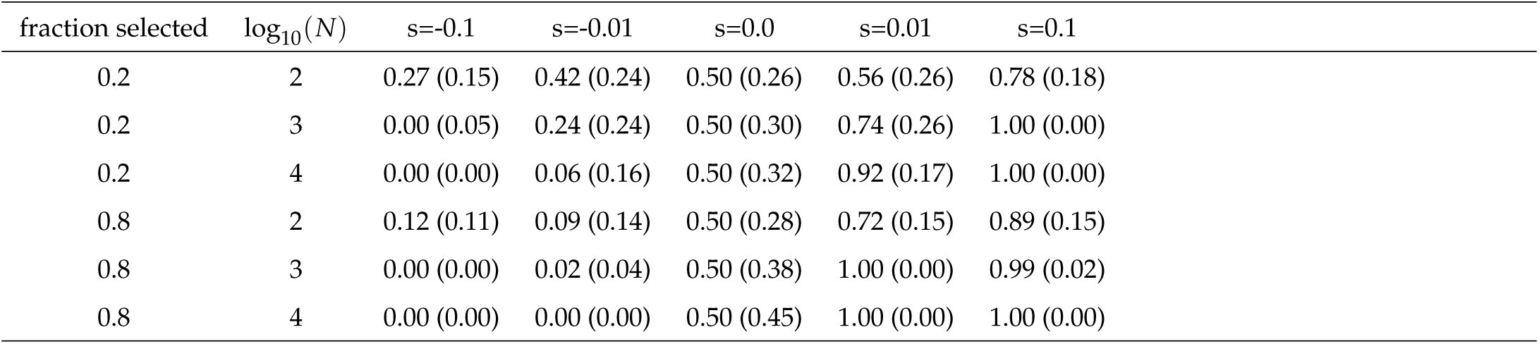
Remarkably, we found the power to infer the population size as well as locus-specific selection coefficients not to be negatively affected under pervasive selection. This is illustrated by comparing the posterior distributions obtained from simulations where 80% of all loci were targeted by selection (Supplementary Fig. 7) to those shown here where only 20% were affected by selection (Fig. 4). More direct evidence is given in Table 1, where we report the posterior probability for s > 0.0 for different combinations of population sizes and selection coefficients and find higher power to identify selected loci under cases of pervasive selection than when only 20% of all loci were simulated under selection.
Table 1: Power to identify loci under selection We report the average and standard deviation (in parenthesis) of the posterior probability obtained under various population sizes and for the cases of 20% and 80% of all loci simulated under selection.
Application to Influenza data
We next applied our approach to publicly available sequencing data of Influenza H1N1 segment 6, obtained at multiple timepoints throughout an evolutionary experiment in which the virus was exposed to an antiviral drug (oseltamivir) (Foll et al. 2014a). While allele frequencies are generally estimated with high accuracy due to the very high coverage in this experiment (about 50,000x), sequencing error may contribute substantially to the observed low frequency variants. In addition, many of the observed mutations likely entered the population only during the experiment, but their exact time of origin is blurred by both the sequencing error as well as sampling. We thus extended our framework to estimate the mutation rate as well as the overall sequencing error rate jointly with the demographic and selection parameters.
We applied our extended method to each of the 8 segments of the Influenza genome individually, but obtained highly concordant results among all segments. As shown in Fig. 5, we infer the effective population size during the experiment to be around 7000, a mutation rate of about 10^−5^ and a sequencing error rate of about 10^−3.8^. While our estimates of the mutation and error rates are consistent with published mutation rates for Influenza (Nobusawa and Sato 2006) and RNA viruses in general (Drake et al. 1998) and also with the employed quality filters on sequencing reads (Foll et al. 2014a), our estimate of the population size is substantially larger than previous estimates of about 225 (Foll et al. 2014a). While we found our approach to slightly overestimate larger population sizes under the spacing of time points relevant here, there are several arguments supporting a larger population size. First, the original estimates were obtained under the assumption of neutrality at all loci, while our approach infers N jointly with selection. Second, the previous estimates were obtained from a small subset of the data, namely the 147 loci with an observed allele frequency ≤ 1% after down sampling to 1000 reads per locus at no less than three timepoints. In contrast, our inference is based on the raw data at the complete set of 13,395 polymorphic loci, including those with small frequencies particularly informative about drift. Third, the original inference accounted for neither sequencing errors nor mutations. In summary, our results argue for a much larger effective population size than previously reported.
Evolution of drug-resistance in Influenza. Here we show the posterior distributions on the population size (log10(N)), sequencing error rate (ϵ), mutation rate (µ) and locus specific selection coefficients sl estimated independently for each of the six segments of the Influenza genome. For the selection coefficients, black dots represent posterior medians and gray lines indicate the 99% credible intervals. Loci for which the 99% credible interval does not include s = 0.0 are shown in red and their actual position within the segment is printed.
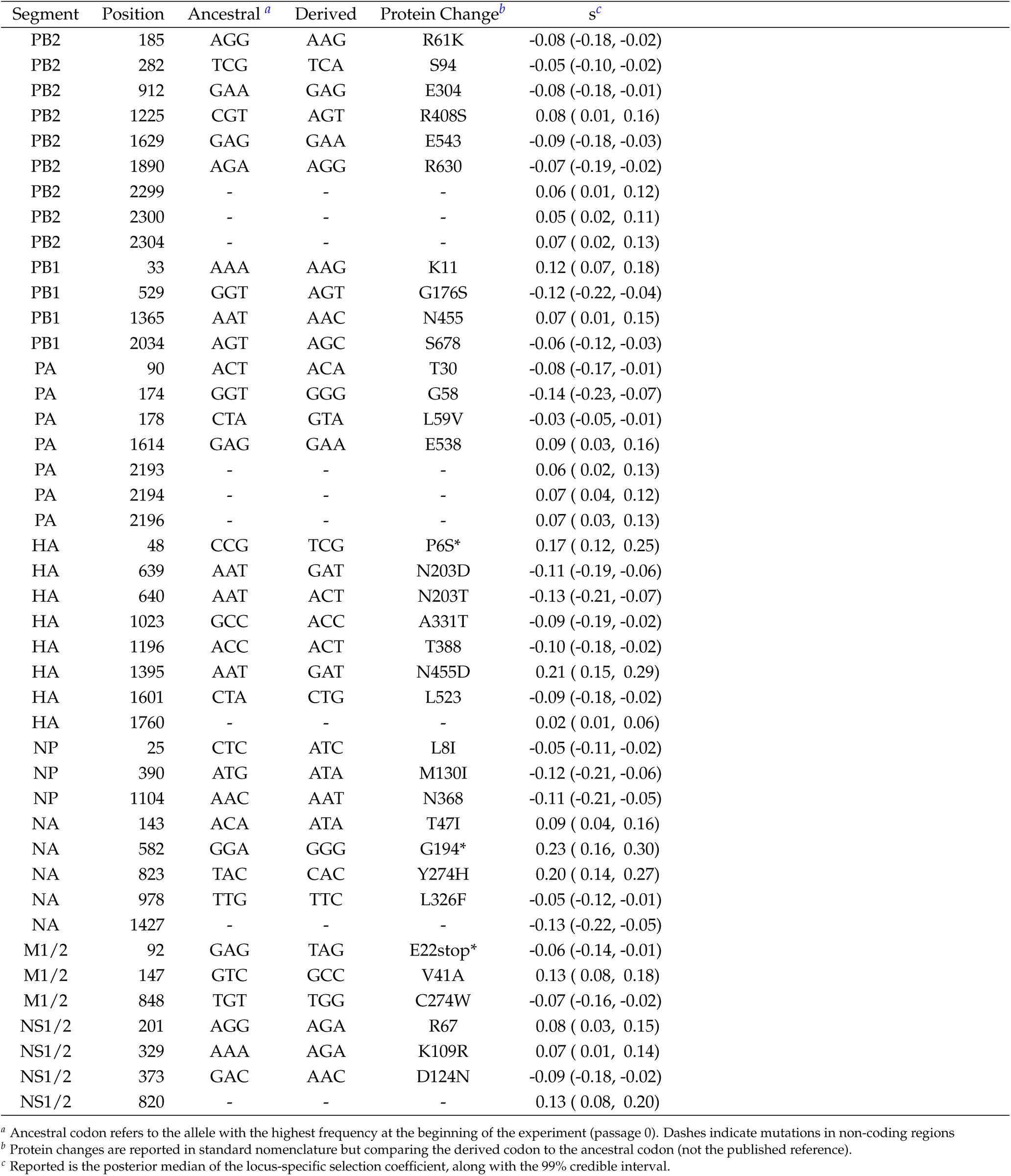
Our results on selection, on the other hand, are highly concordant with previous estimates. In Fig. 5 we report the posterior distributions on the locus-specific selection coefficients for all polymorphic sites for each of the 8 segments of the Influenza genome. As expected, most mutations were found to be selectively neutral or under slight purifying selection (observe the slight asymmetry towards negative selection coefficients for many loci). For a few mutations, however, we found compelling evidence for them to be the target of positive selection (99% credible interval does not include 0). On segment NA, there were three such mutations, of which two stand out with an estimated selection coefficient around 0.2. One of these mutations (Y274H) occurred at a locus at which resistance to oseltamivir has been previously described (Collins et ai 2008). Many additional mutations were found to be the target of selection through out the genome, with many of those likely under negative selection. These are mutations that were found at elevated frequencies at the beginning of the experiment, yet at much lower frequencies after a few passages. The complete list of all mutations found to be under selection is given in Supplementary Table 2.
Conclusion
Here we present a novel, discrete approximation for diffusion processes. This approximation, which we term mean transition time approximation, is designed to preserve the long term behavior of the continuous process it approximates, which renders it particularly suitable to study time series data. Here we derived this approximation for the particular case of inferring selection and demography from such time series data under the classic Wright-Fisher model. As shown through extensive simulations, our approximation is well suited to describe allele trajectories through time, even when only a few states are used. This allowed us to develop a Bayesian inference approach to jointly infer the population size and locus-specific selection coefficients with high accuracy. We further extended this model to further estimate the average sequencing error rate, as well as the per generation mutation rate. We finally applied our approach to data from a recent experiment on the evolution of drug resistance in Influenza virus, identifying likely targets of selection and finding evidence for much larger viral population sizes than previously reported.
The reference list from the paper itself. Each links out to its DOI / PubMed record.
- 1Andolfatto, P. and M. Przeworski, 2000 A genome-wide departure from the standard neutral model in natural populations of Drosophila. Genetics 156: 257–268.
- 2Bollback, J. P., T. L. York, and R. Nielsen, 2008 Estimation of 2Nes from temporal allele frequency data. Genetics 179: 497–502.
- 3Collins, P. J., L. F. Haire, Y. P. Lin, J. Liu, R. J. Russell, P. a. Walker, J. J. Skehel, S. R. Martin, A. J. Hay, and S. J. Gamblin, 2008 Crystal structures of oseltamivir-resistant influenza virus neuraminidase mutants. Nature 453: 1258–61.
- 4Dahlquist, G. and Å. Björk, 2008 Numerical Methods in Scientific Computing. Number v. 1, Society for Industrial & Applied Mathematics.
- 5Drake, J., B. Charlesworth, D. Charlesworth, and J. F. Crow, 1998 Rates of spontaneous mutation. Genetics 148: 1167–1186.
- 6Foll, M., Y.-P. Poh, N. Renzette, A. Ferrer-Admetlla, C. Bank, H. Shim, A.-S. Malaspinas, G. Ewing, P. Liu, D. Wegmann, D. R. Caffrey, K. B. Zeldovich, D. N. Bolon, J. P. Wang, T. F. Kowalik, C. a. Schiffer, R. W. Finberg, and J. D. Jensen, 2014 a Influenza virus drug resistance: a time-sampled population genetics perspective. P Lo S genetics 10: e 1004185.
- 7Foll, M., H. Shim, and J. D. Jensen, 2014 b WFABC: a Wright-Fisher ABC-based approach for inferring effective population sizes and selection coefficients from time-sampled data. Molecular ecology resources pp. 1–12.
- 8Lacerda, M. and C. Seoighe, 2014 Population Genetics Inference for Longitudinally-Sampled Mutants Under Strong Selection. Genetics 198: 1237–1250.