Impulse Control of Multidimensional Jump Diffusions
Mark H.A. Davis, Xin Guo, Guoliang Wu

TL;DR
This paper investigates the regularity of the value function in an infinite-horizon impulse control problem involving multidimensional jump diffusions, showing regularity results similar to diffusion cases despite infinite-activity jumps.
Contribution
It establishes regularity properties of the value function for multidimensional jump diffusions with infinite activity, extending known results from diffusion processes.
Findings
Value function has regularity comparable to diffusion cases.
Regularity holds under certain integrability conditions for jumps.
Results apply to infinite-horizon discounted cost problems.
Abstract
This paper studies regularity property of the value function for an infinite-horizon discounted cost impulse control problem, where the underlying controlled process is a multidimensional jump diffusion with possibly `infinite-activity' jumps. Surprisingly, despite these jumps, we obtain the same degree of regularity as for the diffusion case, at least when the jump satisfies certain integrability conditions.
Click any figure to enlarge with its caption.
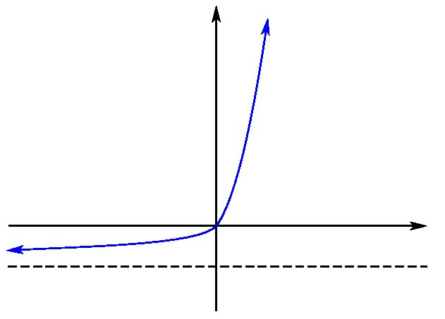 Figure 1
Peer Reviews
No public reviews on file for this paper yet. If you reviewed it on a platform where reviews are public (OpenReview, ICLR, NeurIPS, ICML), you can paste yours below so the community can read it here.
Videos
No videos yet. Explain this paper in a talk, walkthrough, or lecture? Add one.
Taxonomy
TopicsStochastic processes and financial applications · Stability and Controllability of Differential Equations · Mathematical Biology Tumor Growth
Impulse Control of Multidimensional Jump Diffusions
Mark H. A. Davis Department of Mathematics, Imperial College London, London SW7 2AZ, UK. Email address: [email protected]
Xin Guo Department of Industrial Engineering and Operations Research, University of California at Berkeley, CA 94720-1777. Email address: [email protected]
Guoliang Wu Department of Mathematics, University of California at Berkeley, CA 94720-3840. Email address: [email protected]
Abstract
This paper studies regularity property of the value function for an infinite-horizon discounted cost impulse control problem, where the underlying controlled process is a multidimensional jump diffusion with possibly ‘infinite-activity’ jumps. Surprisingly, despite these jumps, we obtain the same degree of regularity as for the diffusion case, at least when the jump satisfies certain integrability conditions.
1 Introduction
This paper is concerned with regularity of the value function in an impulse control problem for an -dimensional jump diffusion process .
In the absence of control, the stochastic process is governed by the following SDE:
[TABLE]
Here is an -dimensional Brownian motion and a Poisson random measure on , with and independent. The Lévy measure may be unbounded and is its compensated Poisson random measure with The parameters satisfy appropriate conditions (see Section 2) to ensure the well-definedness of this SDE.
If an admissible control policy is adopted, then evolves as
[TABLE]
where denotes the Dirac delta function. With this given control, the associated total expected cost (objective function) is
[TABLE]
The aim is to minimize the total cost over all admissible control policies, with the value function
[TABLE]
HJB and Regularity
A heuristic derivation from the Dynamic Programming Principle shows that the value function (1.4) is associated with the following Quasi-Variational-Inequality, or HJB, by
[TABLE]
where is the so called minimal operator such that
[TABLE]
and is the partial integro-differential operator
[TABLE]
where the matrix is given by . Most recently [44] proves rigorously that indeed the value function is a continuous solution to (HJB) in a viscosity sense.
Nevertheless, an important question remains: under what conditions is the value function a solution to the (HJB) in a classical sense? Or, what is the degree of the smoothness (i.e. regularity property) for the value function in general? This is the focus of our paper.
Regularity property has been one of the central topics in PDEs theory [31, 18, 33]. Besides its obvious and natural theoretical interest, regularity study provides useful insight for numerical approximation. Controls of the impulse type by allowing discrete state space and fixed cost proves most desirable for application purpose. See [10, 22, 21, 47] for risk management, [49, 37] for real options, [4, 29, 30, 14, 38, 40] for transaction cost in portfolio management, [26, 7] for insurance models, [35, 6] for liquidity risk, and [27, 39, 8] for optimal control of exchange rates. Meanwhile, jump diffusions such as Lévy processes, have been very popular in financial modeling. See for example [42, 28, 15, 9, 11, 50, 32].
Combined, there is a growing interest and need to analyze impulse controls on jump diffusions. Unfortunately, impulse control is among the hardest to analyze and the regularity study for the associated HJB or the value function is largely open, except for some special and degenerate cases such as singular control and optimal stopping problems, see [36, 43, 19, 2]. One of the difficulty in establishing the regularity property lie in the non-linear, non-local operator in Eqn (HJB), Another difficulty is the partial integro-differential operator associated with the jump processes. For the special case when the controlled diffusion is without jumps, [3] established the regularity property by assuming that the control is bounded and non-negative with additional smoothness in the cost structure. Recently, [20] applies the tricks of translating the regularity of the minimal operator in the action region into that of the PDEs in the continuation region. However, all these technique fail for a controlled jump diffusion component. The major issue is the additional partial integro-differential operator. Moreover, (possibly infinite) jumps through the boundary might potentially reduces the degree of smoothness for the value function.
Our work
This paper investigates the regularity of the value functions for the jump-diffusion models with impulse control. Building on the existence of the viscosity solution to the HJB for the value function [44] and the trick of [20] for the non-local minimal operator, we focus on the partial integro-differential operator in the continuation region. There are two distinct cases: when the jump is driven by compound Poisson process, or equivalently when the Lévy measure is finite, the analysis is fairly straightforward by the standard Schauder’s estimate from PDEs, as in [20]. For the most interesting case of infinite Lévy measure, the key is to combine the classical theory with the “bootstrap” argument to obtain regularity of the partial integro-differential operator. Finally, to deal with the regularity along the “free boundary”, appropriate penalty function is devised. Surprisingly, despite the added possibly infinite jumps, we have here the same regularity as in the diffusion case, at least when the jump satisfies certain integrability conditions.
2 Assumptions and Notations
We first specify the exact mathematical framework for our problem. Given a filtered and complete probability space satisfying the usual conditions, we have a controlled jump diffusion process as defined above at (1.2). An admissible impulse control consists of a sequence of stopping times with respect to and a corresponding sequence of -valued random variables satisfying the conditions
[TABLE]
The associated total expected cost (objective function) is given by (1.4) where is the “running cost”, is the “transaction cost” and is the discount factor. We assume that all the randomness comes from and , so that the filtration is generated by and .
We next specify detailed conditions on the coefficients to ensure the existence and uniqueness of (1.1), as well as the conditions on and in §2.
Throughout this paper, we shall impose the following standing assumptions:
- (A1)
Lipschitz conditions on : there exist constants and a positive function such that
[TABLE]
Assume also that
[TABLE]
- (A2)
Ellipticity: There exists a constant such that
[TABLE]
where the matrix .
- (A3)
Lipschitz condition on the running cost : there exists a constant such that
[TABLE]
- (A4)
Conditions on the transaction cost function :
[TABLE]
- (A5)
.
Assumption (A1) ensures the existence and uniqueness of solutions to (1.1) (Cf. Theorem 9.1, Chapter VI, [23]). The condition (2.2) seems essential to our approach, in particular to establish the continuity property of the operator in Lemma 2. Readers are referred to [17] or [41] for a more detailed discussion of Lévy processes and jump diffusions.
In view of Assumption (A1) the following definitions for operators make sense.
[TABLE]
where and, for Lipschitz continuous functions ,
[TABLE]
We also adopt the following standard notations for function spaces:
[TABLE]
3 Preliminary Results
We first establish some preliminary results under the assumptions (A1)-(A5).
Lemma 1**.**
The value function defined by (1.4) is Lipschitz.
Proof.
Given an admissible control , and two initial states , denote by the solution of (1.1). Apply Itô formula (for jump diffusions) (Theorem 5.1, Chapter II, [23]) to , where ,
[TABLE]
Integrating from 0 to , taking the expectation and then using Assumption (A1), we obtain
[TABLE]
which implies that by Gronwall’s inequality, where . Hence by Assumptions (A3) and (A5), where
[TABLE]
By the arbitrariness of ,
[TABLE]
Exchanging the roles of we get the desired result. ∎
Lemma 2**.**
**
Proof.
Given , , as , for any . Observe that if ,
[TABLE]
where is the Lipschitz constant of . Since and are both -integrable, the dominated convergence theorem yields the desired result. ∎
For reference, we recall here Lemmas 3-5 which were proved in [20].
Lemma 3** (Properties of ).**
**
* is concave: for any and ,*
[TABLE] 2. 2.
* is increasing: for any everywhere,*
[TABLE] 3. 3.
* maps into and maps a Lipschitz function to a Lipschitz function. In particular, is Lipschitz continuous.*
Lemma 4**.**
* and defined as above satisfy for all .*
We define the continuation region and the action region as follows,
[TABLE]
Then, is open, and we have
Lemma 5**.**
Suppose , then
(i) The set
[TABLE]
is nonempty, i.e., the infimum is in fact a minimum.
(ii) Moreover, for any , we have
[TABLE]
in particular,
[TABLE]
4 Viscosity Solutions
There are different ways to define viscosity solutions. Let us begin with the most common one.
Definition 6**.**
A function is called a viscosity subsolution (supersolution, resp.) of (HJB) if whenever has a global maximum (minimum, resp.) at and , we have
[TABLE]
and is called a viscosity solution of (HJB) if it is both a subsolution and a supersolution.
Besides this standard definition of viscosity solutions, there are at least another two different (but equivalent) ones. The second way is to use semijets in stead of test functions. See, for instance, [13] and [44], for more details. For the purpose of proving our regularity results in Section 5, we give a third definition below. The idea is that we impose “local” conditions (rather than global conditions as in Definition 6) on the test functions, and in the equation we only replace by the test function in the “local” terms while still keep in the “nonlocal” terms. The same definition (in different notation) and the proof of equivalence can be found in [45]. See also [46, 1] and [20] for a similar treatment.
Definition 7**.**
A function is called a viscosity subsolution (supersolution, resp.) of (HJB) if whenever has a local maximum (minimum, resp.) at and , we have
[TABLE]
* is called a viscosity solution of (HJB) if it is both a subsolution and a supersolution.*
Theorem 8**.**
The above two definitions of viscosity solutions are equivalent.
Proof.
See [45, Proposition 5.4]. ∎
We now have the following basic result.
Theorem 9** ([41, 44]).**
The value function defined by (1.4) is a viscosity solution of (HJB).
This theorem was proved in [41, Theorem 9.8] as well as [44, Theorem 4.2]111In [44] the result was proved using an in principle smaller class of controls, the so-called ‘Markov controls’. However, this restriction is unnecessary, as can be seen from the proofs of the analogous results in [48] or [25], or [51]. in the sense of our Definition 6. But when we prove the regularity result below, we found it more convenient to use Definition 7. More precisely, by Theorem 8 and Theorem 9, we can “identify” our value function with that of an impulse control problem of diffusion processes without jumps.
Corollary 10**.**
The value function is a viscosity solution of
[TABLE]
where
5 Regularity of Value Function
In this section we study the smoothness of the value function , starting with the special case of a finite Lévy measure.
5.1 Special Case:
Let us first consider the special case in which the Lévy measure is finite, or equivalently, the jump diffusion is driven by a compound Poisson process. Then the operator enjoys the following nice property.
Lemma 11**.**
Suppose , then the operator maps a Lipschitz function to a Lipschitz function.
Proof.
Suppose is Lipschitz with for any , then
[TABLE]
So is Lipschitz. ∎
Corollary 10 and Lemma 11 together imply the regularity of in the continuation region.
Lemma 12** (-Regularity in ).**
Assume that and , then for any compact set , the value function is in the Hölder space for any , and it is a classical solution of
[TABLE]
Proof.
Note that is a viscosity solution of (4.3) by Corollary 10, and hence a viscosity solution of in . On the other hand, for any by Lemma 11. Classical Schauder estimates imply the desired results. (See the proof of Lemma 14 below for a similar argument.) ∎
Finally, an argument as in [20, §4] applies and yields the following
Theorem 13** (-Regularity).**
Assume that and
[TABLE]
Then for any bounded open set and , we have .
5.2 More General Case:
Next, we would like to remove the strong assumption that the Lévy measure is finite, and assume only our standing assumptions (A1)-(A5). Again, we first consider the regularity of in the continuation region , in which the linear elliptic PDE is satisfied. The difficulty is that we do not know is Lipschitz or even Hölder continuous, but only continuous, by Lemma 2.
We cannot apply Schauder estimates at this stage, but the estimates give the following
Lemma 14** (-Regularity in ).**
Assume that , then for any compact set , the value function is in the Sobolev space for any , and it is a strong solution222A strong solution is a twice weakly differentiable function in the bounded domain that satisfies the equation almost everywhere. of
[TABLE]
Proof.
Denote by , which is continuous by Lemma 2. Consider in any open ball the following Dirichlet problem
[TABLE]
Classical theory (Cf. [18, Corollary 9.18]) asserts that the Dirichlet problem (5.2) has a unique strong solution for any , since and the boundary data . Because and , this solution is in fact also a viscosity solution of (5.2) by [24, Theorem 2].
On the other hand, is also a viscosity solution of (5.2) by Corollary 10. Therefore, in by classical uniqueness results of viscosity solutions to a linear elliptic PDE in a bounded domain(Cf. [13, Theorem 3.3]). Hence .
Finally, any compact set can be covered by finitely many balls of radius . Let in the above argument, then is in for all and also in . ∎
With more regularity of in the continuation region , we can use the “bootstrap argument” to obtain further regularity of (and hence ) in .
Theorem 15** (-Regularity in ).**
Assume that , then for any compact set , the value function is in the Hölder space for any , and it is a classical solution of
[TABLE]
Proof.
The key step in the proof is to show for any compact .
Take a compact set such that and . Then by Lemma 12, for any . By Sobolev imbedding, for all . Define the set
[TABLE]
Then for , there is such that
[TABLE]
where is a constant. So or and
[TABLE]
For any ,
[TABLE]
Note that for all and that . Thus the first integral in (5.3) can be estimated by
[TABLE]
for some constant independent of , because by Hölder’s inequality,
[TABLE]
which is a continuous function in and has a maximum on independent of .
The second term in (5.3) can be majored by and the third term is majored by . Thus, putting all three terms in (5.3) together,
[TABLE]
where and are constants independent of . This proves that .
Finally, we can repeat a similar argument in the proof of Lemma 12. This time we know , thus the solution of (5.2) is in fact in by Schauder estimates ([18, Theorem 6.13]). Thus, for compact , and is a classical solution of in . ∎
Parallel to [20], once we have regularity, we are able to obtain regularity for any compact set .
Theorem 16** (-Regularity).**
Assume that
[TABLE]
Then for any bounded open set and , we have . In particular, by Sobolev embedding.
The proof is given in the next section. It follows similar lines to that of [20, Theorem 4.2], involving regularity of an associated optimal stopping problem.
6 Proof of Theorem 16
To study the regularity of the value function for the impulse control problem, we need to investigate the related optimal stopping problem. More precisely, we shall obtain the regularity of solutions for the HJB equation associated with this optimal stopping problem.
Theorem 17**.**
Suppose is a bounded open set in with smooth boundary. Assume
[TABLE]
Assume also that there exist a sequence of functions and a constant satisfying
[TABLE]
If is a viscosity solution of
[TABLE]
then .
Remark 1**.**
Note that Assumption (6.4) is trivially satisfied if . However, later we will apply this theorem to , which is not necessarily in . In applications, can be taken as the usual mollification of , or its slight modification (which may only be in but not in , as in Corollary 18 below).
As a corollary of Theorem 17, we obtain local () regularity of continuous viscosity solutions of
[TABLE]
Corollary 18**.**
Assume that , , and and are Lipschitz in . Assume also that for any bounded open set with smooth boundary, there are constants (maybe depending on ) and such that (6.2) and (6.4) are satisfied.
If is a viscosity solution of (6.6), then for any with smooth boundary and any , and hence also in .
We defer the proofs of Theorem 17 and its corollary to the appendix, and focus now on proving our main theorem using the above corollary.
Proof of Theorem 16.
Given any bounded open set with smooth boundary, we denote by (, resp.) the restriction of the continuation (action, resp.) region within . Then there exists an open ball such that for any , implies Because in this case,
[TABLE]
But as , which implies that all such are bounded uniformly.
Now we define the set
[TABLE]
Clearly, is compact and . From Lemma 12,
[TABLE]
For any , take a minimizing sequence such that . Then . Extract a convergent subsequence (still denoted by ) converging to . Because ,
[TABLE]
Passing to the limit , we obtain
[TABLE]
In particular, .
On the other hand, since is uniformly continuous on , there exists such that
[TABLE]
Hence, for all and unit vector ,
[TABLE]
because
Since for all ,
[TABLE]
and hence the second order difference quotient at
[TABLE]
where .
For simplicity, denote by and its mollification. For any , suppose , then for any , and a unit vector ,
[TABLE]
Sending we get
[TABLE]
Hence,
[TABLE]
where is the -th column of the matrix , is the -th element of and the last inequality is due to continuity of .
Note that and bounded, we deduce
[TABLE]
where the constant is independent of
Finally, recall that is a viscosity of (4.3) by Corollary 10. We can apply Corollary 18 with replaced by and and conclude that for any ,
[TABLE]
∎
Appendix A Proof of Theorem 17
A standard technique to get regularity is to consider a sequence of penalized problems. For this, let denote a sequence of smooth functions satisfying
[TABLE]
Here is the modulus of continuity for the convergence , i.e.,
[TABLE]
Thus, as . For a given , the graph of is shown in Figure 1.
We approximate the Dirichlet problem (6.5) with the following penalizing problems:
[TABLE]
By a standard fixed point argument, (A.2) has a unique solution in , for any . Moreover, we have the following estimates:
Lemma 19**.**
Under the same assumptions as Theorem 17, there exists a constant independent of , such that
[TABLE]
Proof.
The goal is to show that
[TABLE]
Clearly, to get (A.3), it suffices to show
[TABLE]
since by construction.
Consider the point at which the maximum of occurs.
*Case 1. * If , then . Thus
[TABLE]
Because and , we have , if ; or if . In either case, we have at .
*Case 2. * If , then also attains its maximum there, since . By Bony’s maximum principle (see [5] or [34]),
[TABLE]
Thus, either at , which implies , or,
[TABLE]
due to (6.4). By continuity,
[TABLE]
Combing these two cases, we obtain (A.4). Thus, we proved (A.3), and from the PDE (A.2) we have independently of .
Finally, the Calderon-Zygmund estimate implies the desired result. ∎
Thanks to Lemma 19, we can extract a subsequence of , denoted by , such that
[TABLE]
Due to the stability result of viscosity solutions (see, for instance,[12, Theorem 8.3]), this limit function is in fact a viscosity solution of (6.5).
Lemma 20**.**
The limit function is a viscosity solution of (6.5).
Proof.
(Subsolution) Suppose is a smooth test function and has a local maximum at with . We want to show that
[TABLE]
Without loss of generality, we may assume is a strict local maximum because otherwise we can replace by and prove the same result. In this case, for any open ball with radius and centered at , denoted by , has a local maximum for sufficiently large, because converges to uniformly in and . Let go to zero, and we obtain
[TABLE]
By the maximum principle, at . However, satisfies (A.2), thus,
[TABLE]
Note that and locally uniformly, we have
[TABLE]
Sending in (A.5), we obtain
[TABLE]
(Otherwise, at since as if ). Moreover,
[TABLE]
since as if . We have proved that is a viscosity subsolution.
(Supersolution) Similarly, suppose is a smooth test function and has a local strict minimum at with . We want to show that
[TABLE]
For the same reason as above, we can take a sequence so that
[TABLE]
and (A.6) still holds. And again by maximum principle, at ,
[TABLE]
If at , then we have the desired inequality. Otherwise, for some . So for sufficiently large by (A.6), and hence sending in (A.7) yields
[TABLE]
Thus, is a supersolution.
Finally, the boundary condition is satisfied since on . ∎
Proof of Theorem 17.
Because of the above Lemma 20 and the uniqueness of viscosity solutions for (HJB), we conclude that . ∎
Proof of Corollary 18..
To apply Theorem 17, we need to subtract from a function that has the same boundary value on . Let be the unique solution of the Dirichlet problem
[TABLE]
Then . Thus, is a viscosity solution of
[TABLE]
where . Then on . Take , satisfying in . All the other conditions of Theorem 17 are easily verified. So we have and . But since is arbitrary, we have for any . ∎
The reference list from the paper itself. Each links out to its DOI / PubMed record.
- 1[1] G. Barles and C. Imbert. Second-order elliptic integro-differential equations: viscosity solutions’ theory revisited. Ann. Inst. H. Poincaré Anal. Non Linéaire , 25(3):567–585, 2008.
- 2[2] E. Bayraktar and H. Xing. Analysis of the optimal exercise boundary of american options for jump diffusions. SIAM Journal on Mathematical Analysis , 41(2):825–860, 2009.
- 3[3] A. Bensoussan and J.-L. Lions. Impulse Control and Quasivariational Inequalities . Bordas, 1982. Translation of Contrôle Impulsionnel et Inéquations Quasi-variationnelles .
- 4[4] T. Bielecki and S. Pliska. Risk sensitive asset management with fixed transaction costs. Finance and Stochastics , 4:1–33, 2000.
- 5[5] J.-M. Bony. Principe du maximum dans les espaces de Sobolev. C. R. Acad. Sci. Paris Sér. A-B , 265:333–336, 1967.
- 6[6] B. Bruder and H. Pham. Impulse control problems on finite horizon with execution delay. Stochastic Processes and their Applications , 119:1436–1469, 2009.
- 7[7] A. Cadenillas, T. Choulli, M. Taksar, and L. Zhang. Classical and impulse stochastic control for the optimization of the dividend and risk policies of an insurance firm. Mathematical Finance , 16(1):181–202, 2006.
- 8[8] A. Cadenillas and F. Zapatero. Optimal central bank intervention in the foreign exchange market. Journal of Econ. Theory , 97:218–242, 1999.