Detailed discussions and calculations of quantum Regge calculus of Einstein-Cartan theory
She-Sheng Xue

TL;DR
This paper develops a detailed framework for quantum Einstein-Cartan theory using Regge calculus, discretizing space-time with simplicial complexes and holonomy fields, enabling analytical and numerical studies of quantum gravity.
Contribution
It introduces a regularized Einstein-Cartan action on a simplicial complex that respects diffeomorphism and Lorentz invariance, bridging discrete and continuum quantum gravity.
Findings
The regularized action approaches the continuum Einstein-Cartan theory.
The mean-field approximation indicates the 4-simplex size exceeds the Planck length.
Provides a basis for future analytical and numerical quantum gravity research.
Abstract
This article presents detailed discussions and calculations of the recent paper "Quantum Regge calculus of Einstein-Cartan theory" in Phys. Lett. B682 (2009) 300. The Euclidean space-time is discretized by a four-dimensional simplicial complex. We adopt basic tetrad and spin-connection fields to describe the simplicial complex. By introducing diffeomorphism and local Lorentz invariant holonomy fields, we construct a regularized Einstein-Cartan theory for studying the quantum dynamics of the simplicial complex and fermion fields. This regularized Einstein-Cartan action is shown to properly approach to its continuum counterpart in the continuum limit. Based on the local Lorentz invariance, we derive the dynamical equations satisfied by invariant holonomy fields. In the mean-field approximation, we show that the averaged size of 4-simplex, the element of the simplicial complex, is larger…
Click any figure to enlarge with its caption.
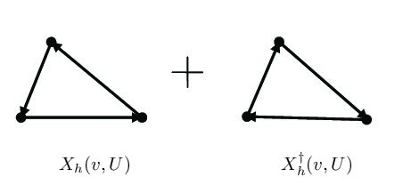 Figure 1
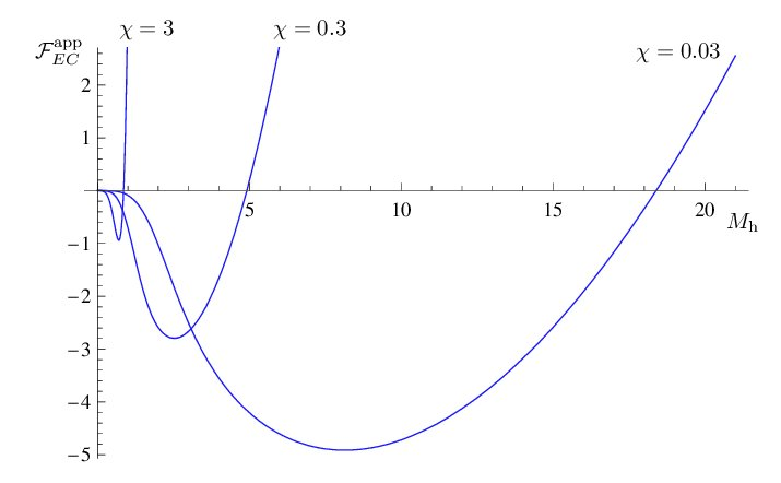 Figure 2
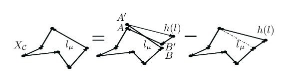 Figure 3
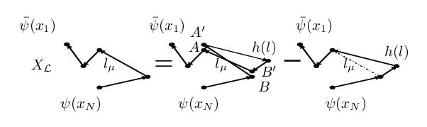 Figure 4
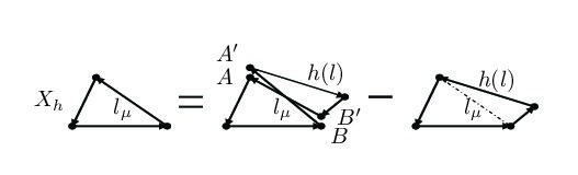 Figure 5
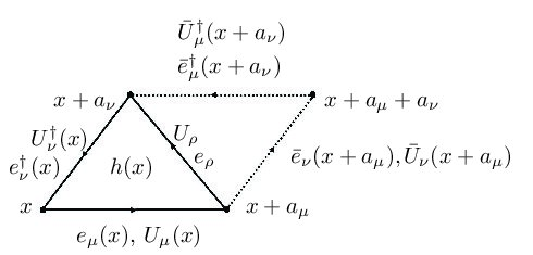 Figure 6
Peer Reviews
No public reviews on file for this paper yet. If you reviewed it on a platform where reviews are public (OpenReview, ICLR, NeurIPS, ICML), you can paste yours below so the community can read it here.
Videos
No videos yet. Explain this paper in a talk, walkthrough, or lecture? Add one.
Detailed discussions and calculations of quantum Regge calculus of Einstein-Cartan theory
She-Sheng Xue
ICRANeT Piazzale della Repubblica, 10-65122, Pescara, Italy
Department of Physics, University of Rome “Sapienza”, Piazzale A. Moro 5, 00185, Rome, Italy
Abstract
This article presents detailed discussions and calculations of the recent paper “Quantum Regge calculus of Einstein-Cartan theory” in Phys. Lett. B682 (2009) 300. The Euclidean space-time is discretized by a four-dimensional simplicial complex. We adopt basic tetrad and spin-connection fields to describe the simplicial complex. By introducing diffeomorphism and local Lorentz invariant holonomy fields, we construct a regularized Einstein-Cartan theory for studying the quantum dynamics of the simplicial complex and fermion fields. This regularized Einstein-Cartan action is shown to properly approach to its continuum counterpart in the continuum limit. Based on the local Lorentz invariance, we derive the dynamical equations satisfied by invariant holonomy fields. In the mean-field approximation, we show that the averaged size of 4-simplex, the element of the simplicial complex, is larger than the Planck length. This formulation provides a theoretical framework for analytical calculations and numerical simulations to study the quantum Einstein-Cartan theory.
pacs:
04.60.Nc,11.10.-z,11.15.Ha,05.30.-d
I Introduction.
Since the Regge calculus regge61 ; wheeler1964 was proposed for the discretization of gravity theory in 1961, many progresses have been made in the approach of Quantum Regge calculus hammer_book ; shamber and its variant dynamical triangulations loll1999 . In particular, the renormalization-group treatment is applied to discuss any possible scale dependence of gravity hammer_book . Inspired by the success of lattice regularization of non-Abelian gauge theories, the gauge-theoretic formulation smolin1979 of quantum gravity using connection variables on a flat hypercubic lattice of the space-time was studied in the Lagrangian formalism. The canonical quantization approaches to the Regge calculus in Hamiltonian formulation are studied in Ref. William1986 . A locally finite model for gravity has been recently proposed thooft2008 . All these studies are very important steps to understand the Einstein general relativity for gravitational fields in the framework of quantum field theory. In the brief paper xue2009 based on the scenario of quantum Regge calculus, we present a diffeomorphism and local Lorentz invariant (i.e., local gauge-invariant) regularization and quantization of Euclidean Einstein-Cartan (EC) theory. Detailed calculations and discussions are presented in this article.
The four-dimensional Euclidean space-time is discretized by a simplicial complex, analogously to the formulation of the Regge calculus. In the framework of the Einstein-Cartan theory, we adopt basic gravitational variables, i.e., a pair of tetrad and spin-connection fields to describe the simplicial complex. Introducing diffeomorphism and local Lorentz invariant (i.e., local gauge-invariant) holonomy fields in terms of tetrad and spin-connection fields along loops, we propose an invariantly regularized EC theory for the dynamics of simplicial complex, which couples to fermion spinor fields. We show that in the continuum limit when the wavelengths of tetrad and spin-connection fields are much larger than the Planck length, this regularized EC action properly approaches to the continuum EC action. The quantum dynamics of the simplicial complex is described by the Euclidean partition function that is a Feynman path-integral overall quantum tetrad, spin-connection, and fermion fields with the weight of regularized EC action. Based on local gauge invariance, we derive the dynamical equations satisfied by invariant holonomy fields of tetrad, spin-connection, and fermion fields. In the mean-field approximation, we show the averaged size of 4-simplex (and its 3-simplex and 2-simplex), elements of the simplicial complex, has to be larger than the Planck length. This formulation provides a theoretical framework for analytical calculations, in particular, numerical simulations to study the Einstein-Cartan theory as a quantum field theory.
This article is organized as follows: In Sec. II, we give a brief review of the continuum EC theory. In Sec. III, we discuss the regularized EC theory based on (1) the description of simplicial complex by tetrad and spin-connection fields; (2) parallel transport equations in simplicial complex; (3) invariant holonomy fields and regularized EC action and their continuum limit; (4) the Euclidean partition function. In Secs. IV and V, we study chiral gauge symmetric bilinear and quadralinear-fermion actions, and derive dynamical equations for holonomy fields. In Sec. VI, we adopt the method of the mean-field approximation to show the averaged size of the 4-simplex has to be larger than the Planck length. In the last section, we give some concluding remarks, and detailed calculations are arranged in Appendices A, B, C, D and E.
II Continuum Einstein-Cartan theory
The basic gravitational variables in the Einstein-Cartan theory constitute a pair of tetrad and spin-connection fields , whose Dirac-matrix values
[TABLE]
The fields and are 1-form real fields on the four-dimensional Euclidean space-time , taking values, respectively, in the local Lorentz vector space and in the Lie algebra of the Lorentz group of the linear transformations of preserving . In this local Lorentz vector space , fermions are spinor fields , Dirac matrices obey
[TABLE]
and (); the Hermitian matrix
[TABLE]
and ; the Hermitian spinor matrix,
[TABLE]
Totally antisymmetric tensor . The space-time metric of four-dimensional Euclidean manifold is
[TABLE]
And the Lorentz scalar components of the metric tensor are then simply
[TABLE]
where the inverse of the tetrad fields and .
Two gauge invariances due to the equivalence principle have to be respected: (1) the diffeomorphism invariance under the general coordinate transformation ; (2) the local gauge invariance under the local Lorentz coordinate transformation , i.e.,
[TABLE]
Under the local Lorentz coordinate transformation (7), the finite local gauge transformation is
[TABLE]
where is the antisymmetric tensor and an arbitrary function of . The Dirac-matrix valued fields , and fermion spinor field are transformed as follows
[TABLE]
where the derivative , the covariant derivative
[TABLE]
and is the gauge coupling. Corresponding to the finite local gauge transformations (9-11), infinitesimal local gauge transformations for fields , and are
[TABLE]
where
[TABLE]
and we use the commutator relation
[TABLE]
to obtain Eq. (15).
In an gauge theory, gauge field can be viewed as a connection on the global flat manifold. On a locally flat manifold, the spin connection , where , one can identify that the spin-connection field or is the gravity analog of gauge field and its local curvature is given by
[TABLE]
and the Dirac-matrix valued curvature . Under the gauge transformation (9,10),
[TABLE]
The diffeomorphism invariance under the general coordinate transformation is preserved by all derivatives and -form fields on made to be coordinate scalars with the help of tetrad fields (see Ref. (wein1972, )). The diffeomorphism and local gauge-invariant EC action for gravity coupling to fermions is given by the Palatini action and host modification for the gravitational field,
[TABLE]
and fermion action (see Refs. art1989 ; kleinert ),
[TABLE]
where , the Newton constant , is the Jacobi of mapping and the integration .
The complex Ashtekar connection A1986 with reality condition and the real Barbero connection b1995 are linked by a canonical transformation of the connection with a finite complex Immirzi parameter i1997 , which is crucial for loop quantum gravity rt1998 .
Classical equations of motion can be obtained by the stationarity of the EC action (21) under variations (9-11),
[TABLE]
From Eqs. (14-16), we find that Eq. (25) can be expressed in terms of independent bases , and of Dirac matrices. Therefore, for arbitrary function , Eq. (25) leads to the following three equalities
[TABLE]
The first and second equations respectively lead to the Dirac equation,
[TABLE]
and the Einstein equation
[TABLE]
where the energy-momentum tensor is
[TABLE]
The gauge invariance of the EC action (21) under the gauge transformation (15) leads to the third constraint equation of Eq. (26), which is the Cartan structure equation,
[TABLE]
where the nonvanishing torsion field,
[TABLE]
relating to the fermion spin current
[TABLE]
The fermion spin-current (32) contributes only to the pseudotrace axial vector of torsion tensor, which is one of irreducible parts of torsion tensor torsion2001 . The solution to Eq. (30) is
[TABLE]
where the connection obeys Eq. (30) for torsion-free case ,
[TABLE]
Replacing the spin-connection field in the Einstein-Cartan action (22,24) by Eq. (34),
[TABLE]
one obtains the well-known Einstein-Cartan theory: the standard tetrad action of torsion-free gravity coupling to fermions with four-fermion interactions,
[TABLE]
Note that the four-fermion interaction actually is the coupling of two fermion spin-currents (32). Taking into account the host action (23), one obtains
[TABLE]
where ar05 . Using the commutator relations (18) and , one can show that is a pseudovector and (40) is invariant under the gauge transformation (11).
As we can see from Eqs. (24) to (39), the bilinear term (24) of massless fermion fields coupled to the spin-connection field (13) is bound to yield a nonvanishing torsion field (30), which is local and static (see, for example, Refs. kleinert ; s2001 ). As a result, the spin connection is no longer torsion-free and acquires a torsion-related spin-connection (34), in addition to the torsion-free spin connection . The torsion-related spin connection is related to the fermion spin current (32). The quadratic term of the spin connection field in the curvature (19) and the coupling between the spin connection field and fermion spin current in Eqs. (13,24) lead to the quadralinear terms of fermion fields in Eqs. (36) and (37). Another way to see this is to treat the static torsion-related spin-connection (34) as a static auxiliary field, which has its quadratic term and linear coupling to the spin current of fermion fields. Performing the Gaussian integral of the static auxiliary field, we exactly obtain the quadralinear term (40), in addition to the torsion-free EC action.
The action (21) and classical Eqs. (27-30) can be separated into left- and right-handed parts lrseparation , with respect to the local and symmetries of the Lorentz group . This can be shown by writing Dirac fermions , where Weyl fermions ; and Dirac-matrix valued tetrad field , , as well as Dirac-matrix valued spin-connection fields , .
III The regularized Einstein-Cartan theory
III.1 Simplicial complex
The four-dimensional Euclidean manifold is discretized as an ensemble of space-time points (vertexes) “” and links (edges) “” connecting two neighboring vertexes. This ensemble forms a simplicial manifold embedded into the . The way to construct a simplicial manifold depends also on the assumed topology of the manifold, which gives geometric constrains on the numbers of subsimplices (, see Ref. loll1999 ). In this article, analogously to the simplicial manifold adopted by the Regge calculus we consider the simplicial manifold as a simplicial complex, whose elementary building block is a 4-simplex (pentachoron). The 4-simplex has five vertexes – 0-simplex (a space-time point “”), five “faces” – 3-simplex (a tetrahedron), and each 3-simplex has four faces – 2-simplex [a triangle ], and each 2-simplex has three faces – 1-simplex [an edge or a link “”]. Different configurations of the simplicial complex correspond to variations of relative vertex-positions , edges “{” and “deficit angles” associating to 2-simplices . These configurations will be described by the configurations of dynamical tetrad fields and spin-connection fields assigned to 1-simplexes (edges) of the simplicial complex in this article. We are not clear now how to relate configurations of fields and to topological constrained configurations of the simplicial complex in dynamical triangulations.
III.1.1 Edges: 1-simplexes
The edge (1-simplex) denoted by , connecting two neighboring vertexes labeled by and , can be represented as a four-vector field , defined at the vertex “” by its forward direction pointing from to and its length
[TABLE]
which is the distance between two vertexes and . The fundamental tetrad field is assigned to each edge (1-simplex) of the simplicial complex to describe the edge location “,” direction “” and length . We use the tetrad field , defined at the vertex , to characterize the edge (1-simplex)
[TABLE]
where the Planck length , and
[TABLE]
By definition, either or is a Dirac-matrix valued four-vector field, defined at the vertex “”.
III.1.2 Triangles: 2-simplexes
We consider an orienting 2-simplex (triangle) (see Fig. 1). This 2-simplex (triangle) has three edges connecting three neighboring vertexes that are labeled by , and . This triangle (2-simplex) has two orientations: (i) the anti-clocklike [] and (ii) the clocklike [].
Along the triangle path of the anti-clocklike 2-simplex [], three edges and their forward directions are represented by: (1) and pointing from to ; (2) and pointing from to ; (3) and pointing from to . The lengths of three edges are respectively represented by edge spacings , and [see Eqs. (41,43)].
We use the tetrad fields
[TABLE]
defined at , and , to respectively characterize locations, forward directions and lengths of three edges: (42) and
[TABLE]
of the anti-clocklike 2-simplex [see Fig. 1 and Eqs. (42, 43)].
III.2 Parallel transports and curvature
The fundamental spin-connection fields are assigned to 1-simplices (edges) of the simplicial complex, i.e., each edge we associate with it . The torsion-free Cartan Eq. (35) is actually an equation for infinitesimal parallel transports of tetrad fields . Applying this equation to the 2-simplex , as shown in Fig. 1, we show that [] undergoes its parallel transport to [] along the () direction for an edge spacing [], following the discretized Cartan equations
[TABLE]
The parallel transports and are neither independent fields, nor assigned to any edges of the simplicial complex. They are related to and fields assigned to the edges and of the 2-simplex by the Cartan Eq. (46,47). Because of torsion-free, and their parallel transports form a closed parallelogram (Fig. 1). Otherwise this would means the curved space-time could not be approximated locally by a flat space-time hrbook . Note that the point at the closed parallelogram (Fig. 1) is not any vertex of the simplicial complex.
For the zero curvature case , the curvature Eq. (19) can be discretized as,
[TABLE]
where and are respectively parallel transports of and in the - and -directions. Analogously to the parallel transports and given by Eqs. (46) and (47), parallel transports and are neither independent fields, nor assigned to any edge of the simplicial complex. They are related to and fields assigned to the edges and of the 2-simplex by the parallel transport Eqs. (48) and (49). The fields and their parallel transports also form a closed parallelogram, analogously to the one formed by the tetrad fields and their parallel transports (see Fig. 1).
Whereas, for the nonzero curvature case , the curvature Eq. (19) can be discretized as
[TABLE]
which define fields and in terms of fields , and curvature . These fields and are neither independent fields, nor assigned to any edge of the simplicial complex. They are related not only to and fields assigned to the edges and of the 2-simplex , but also to the curvature (50) and (51).
These fields and are no longer parallel transports and defined by Eqs. (48) and(49). The difference between and [or between and ] is the curvature [],
[TABLE]
The fields and fields do not form a closed parallelogram, due to the nonzero curvature .
III.3 Group-valued fields
Instead of a field, we assign a group-valued field to each edge (1-simplex) of the simplicial complex. On the edge connecting two vertexes and in the forward direction , we place an group-valued spin-connection fields,
[TABLE]
whereas the same edge in the backward direction , we associate with it
[TABLE]
analogously to the definition of link fields in lattice gauge theories. On the three edges in forward directions , and of the anti-clocklike 2-simplex ( see Fig. 1), we define group-valued spin-connection fields,
[TABLE]
which take values of the fundamental representation of the compact group . On the three edges in backward directions , and of the clocklike 2-simplex (see Fig. 1), we define group-valued spin-connection fields,
[TABLE]
These uniquely define group-valued spin-connection fields on the anti-clocklike and clocklike 2-simplex.
III.3.1 Unitary operators for parallel transports of fields
Actually, these group-valued fields (56-58) and (59-61) can be viewed as unitary operators for finite parallel transportations. The parallel transportation (Cartan) Eqs. (46) and (47) can be generalized to
[TABLE]
and using Eq. (55) these equations can be equivalently rewritten as
[TABLE]
While for , we similarly have the following parallel transportation equations
[TABLE]
indicating that is parallel transported to in the forward direction, and is parallel transported to in the backward direction. Similar discussions can be made for parallel transports with the unitary operator .
III.3.2 Unitary operators for parallel transports of fields
In the simplicial complex, each edge (1-simplex) connecting two vertexes has only one direction. One can identify each edge by its starting vertex and direction pointing to its ending vertex. On the basis of the tetrad field (42) defined at the vertex “” for the edge () starting from the vertex “” in the forward direction () to the vertex “,” below, using the unitary operator for parallel transports, we will uniquely introduce the “conjugated” field defined at the vertex “” to describe the same edge () but in the backward direction starting from the vertex “” to the vertex “.” Analogously to Eq. (42), this edge starting from the vertex “” in the backward direction () can be formally represented by
[TABLE]
By the parallel transport, we define the field as
[TABLE]
in terms of the unitary operator and conjugated tetrad fields defined at the vertex “”. From the definition in Eq. (68), we rewrite
[TABLE]
The second equalities in Eq. (68) and Eq. (69) are given by the definition of parallel transports by unitary operators [see Eq. (62)]. Equation (68) means that we can associate the conjugated field
[TABLE]
with the same edge but in backward direction and write
[TABLE]
As a result, the edge () [()] in the forward (backward) direction is uniquely described by the field [] defined at the vertex . Note that the conjugated field is given by the parallel transport (70) from to in the direction . In addition, Eqs. (68) and (69) indicate that conjugated fields mean the inverse of field’s direction .
This prescription shows that the edge () is completely described by the fields and , latter is a function of fields and , as required by the principle of local gauge symmetries and the gauge field corresponds a parallel transport between and . In consequence, any edge (1-simplex) of the simplicial complex is uniquely identified by its location and direction (), and described by the fields and .
Using the properties [see Eq. (2)] and the definition of tetrad field , where the index is fixed, we have
[TABLE]
where because of the index being fixed, the real tetrad-field component can be viewed as a one-row matrix and a one-column matrix .
Analogously to Eq. (43), the length of the edge (71) in backward direction ,
[TABLE]
which is the same as the length of the edge in the forward direction .
We turn to the discussion of other two backward-direction edges and of the clocklike 2-simplex (see Fig. 1). Analogously to Eqs. (68,69), we have in the direction,
[TABLE]
and in the direction
[TABLE]
As a result, the edge () [()] in the forward (backward) direction is uniquely described by the field [] defined at the vertex
[TABLE]
see Eq. (74). Note that the conjugated field is given by the parallel transport (76) from to in the direction . We can write
[TABLE]
Similarly, the edge () [()] in the forward (backward) direction is uniquely described by the field [] defined at the vertex
[TABLE]
see Eq. (75). Note that the conjugated field is given by the parallel transport (78) from to in the direction . We can write
[TABLE]
This prescription shows that the edge () is completely described by the fields and , and the edge () by the fields and . The field [] corresponds a parallel transport between and ( and ).
Along the triangle path of the clocklike 2-simplex [] (see Fig. 1), these three edges and their backward directions are formally represented by (1) and pointing from to ; (2) and pointing from to ; (3) and pointing from to . Based on Eqs. (68), (74), (75), (70), (76) and (78), we use the conjugated tetrad fields
[TABLE]
which are respectively defined at vertexes , , ,
to characterize both backward directions and lengths of three edges (71), (77), and (79) of the clocklike 2-simplex .
In the simplicial complex, each edge (1-simplex), described by tetrad field , is uniquely identified by its location and direction (), and each triangle (2-simplex) has a definite orientation, as indicated in Fig. 1, either anti-clocklike or clocklike. Thus each triangle, for example, the one presented in Fig. 1 is completely described by the tetrad fields , , , and unitary operators , , .
III.3.3 Unitary operators and curvature
In the zero curvature case, the group-valued fields for parallel transports and , defined by parallel transport Eqs. (48) and (49), are given by
[TABLE]
Similarly to Eqs. (62,63), the parallel transport Eqs. (48) and (49) can be generalized to
[TABLE]
The parallel transport fields and together with and form a closed parallelogram, see Fig. 1. This closed parallelogram is not the same as the parallelogram formed by and fields.
In the nonzero curvature case, corresponding to the fields and defined by Eqs. (50) and (51), the group-valued fields can be similarly given by
[TABLE]
whose values obviously depend on the curvature . The same as the fields and , these group-valued fields and are neither independent fields, nor assigned to any edge of the simplicial complex. They are related to and fields assigned to the edges and of the 2-simplex by
[TABLE]
which are generalized from Eqs. (50) and (51). The fields and defined in Eqs. (85,86) encode the information of a nontrivial curvature. They do not form a closed parallelogram together with and , at the point (see Fig. 1).
In order to see the nontrivial curvature information encoded in the fields and defined by Eqs. (84)-(86), based on Eqs. (85) and (86), we introduce quantities
[TABLE]
and calculate their expressions in the naive continuum limit. In the naive continuum limit: (small coupling or weak field), indicating that the wavelengths of weak and slow-varying fields are much larger than the edge spacing , we obtain (see Appendix A)
[TABLE]
where indicates high-order powers of . It is shown that the quantity [Eq. (89)] is related to the curvature in Appendix A. For the sake of simplicity in the following calculations to show the naive continuum limit, the quantities introduced by (87) and (88) and their expressions in the naive continuum limit (89) are useful.
III.4 Triangle constrain and area
Three tetrad fields , and [see Eq. (44)] are three edges of the anti-clocklike 2-simplex , satisfying the triangle constraint
[TABLE]
Equivalently, three tetrad fields , and [see Eqs. (70), (76), and (78) or (80)] of the clocklike 2-simplex , satisfying the triangle constraint
[TABLE]
where [see Eq. (75)]. Also, Eq. (74) is used for in the second equality of Eqs. (90,91). Two of three edges are independent for a given anti-clocklike (clocklike) 2-simplex [].
However, in Eqs. (90,91), vector fields defined at different vertexes are related without being parallel transported to the same vertex, thus these relationships are not proper and does not properly transform under local gauge transformations. This is an exactly essential point of local gauge symmetries, that gauge fields for parallel transports are needed to relate variations of gauge freedom at different coordinate points. Using the parallel transport by the unitary operator , we rewrite the triangle constraint (90) for the anti-clocklike 2-simplex as
[TABLE]
where in the left-handed side, is parallel transported from the vertex to the vertex to be related to and at the same vertex in the right-handed side. Using , we rewrite Eq. (92) as
[TABLE]
Using the parallel transport by the unitary operator , we rewrite the triangle constraint (91) for the clocklike 2-simplex as
[TABLE]
where in the left-handed side is parallel transported from the vertex to the vertex to be related to and at the same vertex in the right-handed side. Equation (94) is identical to Eq. (92) or Eq. (93), if we consider and . The proper parallel transports by unitary operators can shift the triangle constrain to other vertexes for example, and .
We are now in the position of discussing the area of the 2-simplex . We define the fundamental area operator of the anti-clocklike 2-simplex (see Fig. 1)
[TABLE]
at the vertex . In addition, we can also define the following area operators
[TABLE]
at the vertex , and
[TABLE]
at the vertex . Using Eqs. (68), (74), and (75), we rewrite the area operators (95)-(97) of the anti-clocklike 2-simplex as
[TABLE]
In the following, we show that area operators (98)-(100) defined at three vertexes , , and are universal up to parallel transports by unitary operators. Using Eqs. (68) and (92), we obtain
[TABLE]
Analogously, using Eqs. (74) and (94), we obtain
[TABLE]
In Eqs. (101) and (102), we use , and the same for . This shows that the area operators (98), (99) and (100) defined at three vertexes of the 2-simplex are universal up to parallel transports.
Therefore, Eq. (95) or (98) defines the area operator of the 2-simplex
[TABLE]
up to parallel transports. As consequence, the area of the 2-simplex is uniquely determined by
[TABLE]
Its uniqueness [independence of the vertexes , and of the 2-simplex ], i.e.,
[TABLE]
can be shown by using Eqs. (101,102).
In the same way as Eqs. (95)-(97), we define the area operators of the clocklike 2-simplex :
[TABLE]
whose directions are opposite to the counterparts of anti-clocklike 2-simplex . However, the area of the clocklike 2-simplex is equal to the area (104).
Based on the definition of 2-simplex area (104), we can define a volume element around the vertex “”
[TABLE]
where indicates the volume element contributed from a 2-simplex , and indicates the sum over all 2-simplices that share the same vertex . This definition of volume element (107) indicates that a 2-simplex contributes the volume element at its three vertexes , and .
Before ending this section, we note that using the parallel transports (68), (74), and (75), one can obtain parallel transports of area operators (95,96,97) of triangles (2-simplexes),
[TABLE]
which are consistent with the definitions of unitary operators and for parallel transports (62,63) of edges (1-simplexes). The notation “” instead of in the left-handed side of Eqs. (III.4) indicates that the parallel transport “” is not associated to any triangle of the simplicial complex.
III.5 Local gauge transformations
In accordance with Eq. (10), the bilocal gauge transformations of three fields (56)-(58) of the anti-clocklike 2-simplex are,
[TABLE]
and their inverses (59)-(61) of the clocklike 2-simplex transform as
[TABLE]
In accordance with Eq. (9), the tetrad fields and for the anti-clocklike 2-simplex transform under local gauge transformations
[TABLE]
respectively at the vertexes , and where they are defined. Using above local gauge transformations (109)-(111), we obtain the following local gauge transformations of the conjugated fields , and defined by Eqs. (68), (74), and (75) for the clocklike 2-simplex ,
[TABLE]
These local gauge transformations (112) of the conjugated fields at the vertexes , and are in the same manner as that given by Eqs. (111). This means that each edge (1-simplex) of the simplicial complex is uniquely described by tetrad fields and , that are defined at the vertex , and covariantly transformed under local gauge transformation.
It is worthwhile to mention that the transformations (112) are just conjugated transformations (111), and consistent with
the following local gauge transformations:
[TABLE]
which follow the transformation rules of Eq. (111).
It is shown that the tetrad fields (44) and their conjugated fields (80) given by Eqs. (70), (76), and (78), as well as the triangle constraints (92,94), are gauge covariant, and properly transformed under local gauge transformations (109)-(112). The length (43) or (73) of edges (1-simplexes) is unique and invariant under local gauge transformations (109)-(112).
Under local gauge transformations (109)-(112), the fundamental area operators (98)-(100) of the anti-clocklike 2-simplex are gauge covariant and transform
[TABLE]
which are consistent with Eqs. (101), (102), (109), and (110), and their counterparts [see Eq. (III.4)] of the clocklike 2-simplex transform in the same manner. The parallel transports (III.4) of area operators transform consistently with Eqs. (109), (110) and (114). However, the area (104) of the 2-simplex is unique and invariant under local gauge transformations.
It is worthwhile to mention that under local gauge transformation (109)-(111), parallel transport fields (62) and (63) transform locally
[TABLE]
in accordance with local gauge transformations (111) for tetrad fields. Therefore, the closed parallelogram (see Fig. 1), formed by and their parallel transports , is invariant under local gauge transformation. This is consistent with the torsion-free condition for the existence of local Lorentz frames at each points of a curved space-time.
The prescription of using tetrad fields and gauge fields for parallel transports to describe edges (1-simplexes) and triangles (2-simplexes) of the simplicial complex fully respects the principle of local gauge symmetries. Therefore, this prescription is independent of a particular vertex , oriented edge and triangle , because of the gauge invariance. The formulation of defining tetrad fields at one of edge endpoints “” and direction “,” and each triangle has a definite orientation is gauge invariant.
However, the gauge transformation properties of fields and defined by Eqs. (85) and (86), as well as and introduced by Eqs. (87) and (88), are very complicate under the bilocal gauge transformations (109) and (110). This implies that we could not use these fields to construct a gauge-invariant object. We need to study the object of three fields, , and along a closed triangle path of each 2-simplex (see Fig. 1), which will be discussed in the next section.
III.6 Regularized EC action
To illustrate how to construct a gauge-invariantly regularized EC theory describing dynamical configurations of the simplicial complex, we consider anti-clocklike 2-simplex (triangle) and clocklike 2-simplex (triangle) (see Fig. 1 and Fig. 2).
For simplifying notations, we henceforth do not explicitly write negative signs to indicate the backward directions of edges. In terms of the tetrad fields and of the 2-simplex (see Fig. 1), we introduce the following vertex fields :
[TABLE]
which have properties: , and (see Appendix B). Under the local gauge transformation (9,111), the vertex fields (116) and (117) transform locally at a vertex ,
[TABLE]
which is transformed in the same manner as area operators (114). In addition to the vertex field (117) at the vertex , we can define in the same way the vertex fields at the vertex , and at the vertex of the anti-clocklike 2-simplex (see Fig. 1). Actually, the vertex fields (117), and are related to the fundamental area operators (98), (99) and (100), e.g.,
[TABLE]
As discussions for three area operators in Eqs. (95)-(103), only one of three vertex-fields , and is independent for the anti-clocklike 2-simplex . As for an clocklike 2-simplex , vertex fields can be obtained by using the relations and .
Using the tetrad fields and vertex fields to construct coordinate and Lorentz scalars to preserve the diffeomorphism and local gauge invariance, we define a smallest holonomy field along the closed triangle path of the 2-simplex (see Fig. 1):
[TABLE]
whose orientation is anti-clocklike, as shown the left graphic in Fig. 2. Considering the clocklike orientation, as shown the right graphic in Fig. 2, we have
[TABLE]
On the other hand,
[TABLE]
where in the second line of equation, we use the properties , , and . Therefore we have
[TABLE]
Equations (121)-(123) are invariant under gauge transformations (109), (110), and (118).
Using Eqs. (120)-(123), we are ready to construct the diffeomorphism and local gauge-invariant regularized EC action. First we consider the case :
[TABLE]
where is the sum over all 2-simplices of the simplicial complex. In the naive continuum limit: , Eq. (124) becomes (see Appendix B)
[TABLE]
where the 2-simplex contributed volume element is given in Eq. (104) or Eq. (225).
Based the volume element (107) around the vertex “”
[TABLE]
where stands for a sum overall vertexes (0-simplices) of the simplicial complex, and the factor is due to each 2-simplex contributing its area to its three vertexes. The interior of the 4-simplex is approximately flat, leading to
[TABLE]
As a result, Eq. (125) approaches to (22) with an effective Newton constant
[TABLE]
and . The second we consider the case :
[TABLE]
where the real parameter [see Eq. (23)]. Analogously, in the naive continuum limit: , Eq. (129) approaches to (23) [see Appendix B],
[TABLE]
with the effective Newton constant (128). The diffeomorphism and local gauge-invariant regularized EC action is then given by
[TABLE]
In addition, we can generalize the link field to be all irreducible representations of the gauge group . The regularized EC action (131) should be a sum over all irreducible representations ,
[TABLE]
where is the dimensions of the irreducible representations and for the fundamental representation, which is the dimension of the Dirac spinor space.
III.7 Invariant holonomy fields along a large loop
We consider the following diffeomorphism and local gauge-invariant holonomy fields along a loop on the Euclidean manifold
[TABLE]
where is the path-ordering and “” denotes the trace over spinor space. We attempt to regularize these holonomy fields (133) on the simplicial complex . Suppose that an orientating loop passes space-time points (vertexes) and edges connecting between neighboring points in the simplicial complex (see the diagram in the left-hand side of graphic equation, Fig. 4). At each point two tetrad fields and respectively orientating path incoming to () and outgoing from () the point , we have the vertex field defined by Eqs. (116) and (117). Link fields are defined on edges lying in the loop . Recalling the relationship [see Eqs. (59-61)], we can write the regularization of the holonomy fields (133) as
[TABLE]
which preserve diffeomorphism and local gauge invariances. The holonomy fields are functionals of fields () and loop . Consistently with the holonomy fields [Eq. (134)], the holonomy field [Eq. (120)] is the one with the smallest loop, i.e., the closed path of the 2-simplex (triangle) , see Fig. 1.
III.8 Euclidean partition function
The partition function and effective action are given by
[TABLE]
with the diffeomorphism and local gauge-invariant measure
[TABLE]
where indicates the product of overall edges (1-simplices) of the four-dimensional simplicial complex . As already mentioned, the configuration is formulated such that each edge is defined by giving its coordinate (vertex) in one of the endpoint coordinates and , and giving its forward direction pointing from to . This endpoint coordinate and forward direction have to be uniquely chosen for each edge . Beside, on such defined edge , we place an independent gauge field corresponding a parallel transport between and . The gauge invariant properties, discussed in Sec. III.5, guarantee that the change of a formulation does not lead to the change in the measure of the configuration . In addition, the triangle constraint (92) and (93) must be imposed in the measure (136), symbolically indicated as , a functional of Eq. (92) or Eq. (93).
In the single edge measure [see Eq. (136)]
[TABLE]
is the invariant Haar measure of the compact gauge group or , and is the measure of the Dirac-matrix valued field , determined by the functional measure of the bosonic field . The single edge measure has to be the measure over fields only and of the edge in the forward direction , because and of the edge in the backward direction are related to the fields and by Eqs. (55), (68), (70), and (72) so that the single edge measure (137) is actually over all degrees of fields assigned on the edge.
It should be mentioned that the measure (136) is just a lattice form of the standard DeWitt functional measure dewitt67 over the continuum degrees, with the integral of the spin-connection field replaced by the Haar integral over the ’s, analytical integration or numerical simulations runs overall configuration space of continuum degrees and no gauge fixing is needed. In addition, it should be noted that the measure (136) does not contain parallel transport fields and , for examples and (see Fig. 1) given by the Cartan Eqs. (46) and (47), since parallel transport fields are not associated to any edges of the four-dimensional simplicial complex. This means that the torsion-free Cartan equation has been taken into account.
In this path-integral quantization formalism, the partition function (135) presents all dynamical configurations of the simplicial complex, described by the configurations of dynamical fields and in the weight of . The effective action (135) contains all one-particle irreducible (1PI) functions(operators), i.e., all truncated -point Green-functions. The vacuum expectational values (v.e.v.) of diffeomorphism and local gauge-invariant quantities, for instance holonomy fields (134), are given by
[TABLE]
In the action (124,129), [Eq. (120)] contains the quadratic term of -field associated to each edge of 2-simplex , the partition function (135) and v.e.v. (138) are not divergent for large fluctuating fields, provided the action is positive definite, see discussions below. On the other hand, all edge lengths do not vanish [, see Eqs. (41,42)], and all simplicial triangle inequalities and their higher dimensional analogs should be imposed wheeler1964 ; hammer_book . Integrating spin-connection fields over the Haar measure of compact gauge groups is similar to that in the Wilson-lattice QCD, the difference is that the (120) contains three fields in a 2-simplex , while the Wilson action contains four fields in a plaquette. Equation (138) can be calculated by numerical Monte-Carlo simulations. We are trying do some numerical Monte-Carlo simulations, it will take time so that the results will be published in a separate paper.
Before ending this section, we make some discussions on the convergences of the partition function (135) and v.e.v. (138). Suppose that we first integrate Eqs. (135) and (138) over the compact Haar measure of the gauge group, roughly speaking, the result gives, in addition to a polynomial of tetrad fields , a combination of both decreasing exponents and increasing exponents as functions of increasing tetrad fields . From the regularized action (120), one can find that depend on 2-simplex area operators (104) and are the sum over all 2-simplexes. are either some extremal values of the action (131) with respect to group-valued fields, or those values taken at the boundary points of the compact gauge group. Clearly, for the case of decreasing exponents , integrations Eqs. (135) and (138) over tetrad fields are convergent. This is certainly the case for perturbative weak fields, i.e., . While for the case of increasing exponents , integrations Eqs. (135) and (138) over tetrad fields are divergent.
To avoid these possible divergences, it is necessary to add into the regularized action (131) an additional term of another dimensionality: either a curvature squared term: with a new coupling parameter; or a bare cosmological term: . We consider here an additional bare cosmological term to the regularized action (131): ,
[TABLE]
where the cosmological parameter and is the bare cosmological constant. The bare cosmological term is a four-dimensional volume term (sum over all vertexes ), which is independent of configurations of group-valued fields. The exponent decreases with strong tetrad fields , large volume configurations. Bare parameters , and play an important role for convergences of the partition function (135) and vacuum expectational values (138). It needs further studies to find the region of bare parameters , and for the convergences, and the scaling invariant region () for the physically sensible continuum limit, see the discussions in the last Sec. VII.
III.9 Local** gauge symmetry**
Analogously to Eq. (25), the local gauge invariance of the partition function (135), i.e., under the gauge transformation (109) and (118), leads to (no summation over index )
[TABLE]
Based on and (14) and (15) for an arbitrary function and the independent bases of Dirac matrices , and , we obtain the “averaged” Cartan Eq. (35) for the torsion-free case,
[TABLE]
where we use
[TABLE]
for the group-valued field (56). The averaged torsion-free Cartan Eq. (141) actually shows the impossibility of spontaneous breaking of the local gauge symmetry. This should not be surprised, since the torsion-free (30) is a necessary condition to have a local Lorentz frame, therefore a local gauge-invariance, as required by the equivalence principle.
IV Including fermion fields
IV.1 Bilinear and quadralinear-fermion actions
Introducing dimensionless fermion field (drop “prime” henceforth) and using the relations , and
[TABLE]
we consider the following regularized kinetic action of fermion fields,
[TABLE]
where fermion fields and are defined at two neighboring points (vertexes) of the edge , (see Fig. 1), where fields and are added to preserve local gauge and diffeomorphism invariances, and is the sum over all edges (1-simplexes) of the simplicial complex.
Using Eq. (142) and performing a variation of the regularized fermion action (144) with respect to the spin-connection field , i.e., , we obtain the nonvanishing torsion field , where the regularized fermion spin current is
[TABLE]
[see Eq. (32)]. Instead of solving regularized Cartan equation and finding an effective theory, as what is done in the continuum case (25)-(32), we assume that the in Eqs. (144) and (145) is the group-valued spin-connection field for the torsion-free case (35), i.e., . Thus, the regularization of the effective EC theory (39) and (40) is given by Eqs. (131) and (144) and the regularized four-fermion interaction
[TABLE]
where [see Eq. (40)]. In the naive continuum limit , the regularized fermion action (144) approaches to the continuum fermion action (24), and Eqs. (145) and (146), respectively approach to their continuum counterparts (32) and (40).
The diffeomorphism and local gauge-invariant regularized EC action is then given by
[TABLE]
The partition function and effective action are
[TABLE]
with the diffeomorphism and local gauge-invariant measure
[TABLE]
where is the measure of Grassmann anticommuting fields. Analogously to Eq. (132), Eqs. (147)-(149) can be straightforwardly generalized to include all irreducible representations of the gauge group that couple to corresponding spinor states of fermion fields.
IV.2 Holonomy fields with fermions
We consider the following diffeomorphism and local gauge-invariant quantities
[TABLE]
where stands for an orientating () path connecting two vertexes and () on the simplicial complex . In Eq. (150), represents the evolution of the spin of fermion fields from the vertex to the vertex under the gravitational field influence. Analogously to discussions in Sec. (III.7) for the holonomy fields (133), we regularize these quantities (150) on the simplicial complex as follows:
[TABLE]
which preserves diffeomorphism and local gauge invariances. The graphic representation of