
TL;DR
This paper investigates coefficients related to the Riemann zeta function's nontrivial zeros, providing new relations, representations, and asymptotic behavior under the Riemann hypothesis.
Contribution
It introduces novel expressions and integral representations for coefficients linked to zeta zeros, advancing understanding of their properties and asymptotics.
Findings
Expressed $b_n$ as sums over zeta zeros
Derived integral representations of $b_n$
Established asymptotic form $b_n o 2^{-n-2} abla n$ under RH
Abstract
We study coefficients that are expressible as sums over the Li/Keiper constants . We present a number of relations for and representations of . These include the expression of as a sum over nontrivial zeros of the Riemann zeta function, as well as integral representations. Conditional on the Riemann hypothesis, we provide the asymptotic form of .
Click any figure to enlarge with its caption.
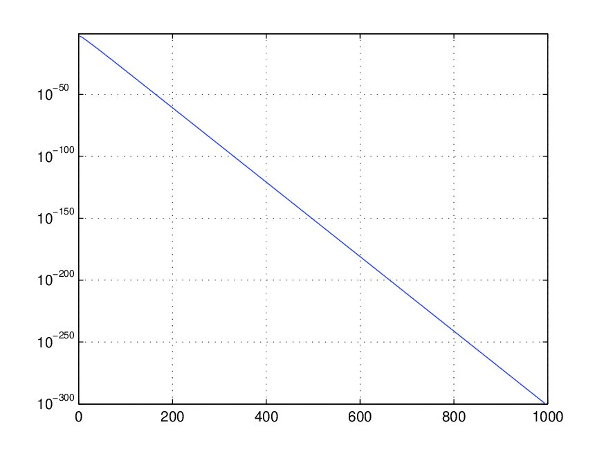 Figure 1
| 0 | -0.698922 |
|---|---|
| 1 | 0 |
| 2 | 0.00144406 |
| 3 | 0.00144406 |
| 4 | 0.00108297 |
| 5 | 0.000721886 |
| 6 | 0.000451088 |
| 7 | 0.00027058 |
| 8 | 0.000157786 |
| 9 | 0.0000901269 |
| 10 | 0.0000506726 |
| 11 | 0.0000281364 |
| 12 | 0.0000154657 |
| 13 | |
| 14 | |
| 15 | |
| 16 | |
| 17 | |
| 18 | |
| 19 | |
| 20 | |
| 21 | |
| 22 | |
| 23 | |
| 24 | |
| 25 |
Peer Reviews
No public reviews on file for this paper yet. If you reviewed it on a platform where reviews are public (OpenReview, ICLR, NeurIPS, ICML), you can paste yours below so the community can read it here.
Videos
No videos yet. Explain this paper in a talk, walkthrough, or lecture? Add one.
On certain sums over the nontrivial zeta zeros
Mark W. Coffey
Department of Physics
Colorado School of Mines
Golden, CO 80401
(Received 2009)
(October 2, 2009)
Abstract
We study coefficients that are expressible as sums over the Li/Keiper constants . We present a number of relations for and representations of . These include the expression of as a sum over nontrivial zeros of the Riemann zeta function, as well as integral representations. Conditional on the Riemann hypothesis, we provide the asymptotic form of .
Key words and phrases
Riemann zeta function, Li criterion, Li/Keiper constants, Riemann hypothesis, functional equation, nontrivial zeros, integral representation, asymptotic form
MSC numbers
11M06, 11M26, 11Y60
Introduction
Let denote the Riemann zeta function, and the classical completed zeta function, where is the Gamma function [9, 12, 16, 17]. Within the critical strip , , the complex zeros of and coincide, and we denote them by . The -function is entire, of order , and of maximal type.
Herein, we mainly investigate certain sums over complex zeta function zeros. We provide various representations and properties of these sums. We also supply some remarks on the Li criterion [14] for the Riemann hypothesis (RH).
We recall that the Li equivalence for the RH results as a necessary and sufficient condition that the logarithmic derivative of the function be analytic in the unit disk. This obtains from a conformal map of the critical strip to this disk. The equivalence [14] states that a necessary and sufficient condition for the nontrivial zeros of the -function to lie on the critical line Re is that constants are nonnegative for every integer . The sequence can be defined by
[TABLE]
The ’s are connected to sums over the nontrivial zeros of by way of [13, 14]
[TABLE]
For further discussion of the Li criterion, its application, and results on series expansion of the function, see for instance [2, 4, 5, 6, 3, 7].
In particular, consider the expansions [11]
[TABLE]
The middle expansion in terms of the Li/Keiper constants holds for , where corresponds to the Riemann hypothesis. Similarly, the right-most expansion holds for . Thus, (1.3) has overlapping domains of expansion, allowing analytic continuation.
In [11], the coefficients of (1.3) are simply an inessential device. However, we treat their properties, including a “curious identity” , in the next section. The latter relation is simply the beginning of an infinite set of relations that we make explicit. In the Appendix, we record approximate numerical values for the early coefficients. Reference [11] contains physical discussion, including attempting to regard as a quantum mechanical wave function.
To emphasize that the ’s are not required for the purposes of [11], we have the following argument. Let be the count of nontrivial zeta zeros for . We have , and it is well known that as , . Suppose that the RH holds. Then we have
[TABLE]
where or . We can rewrite (1.4) as
[TABLE]
where the lower limit just as well may be taken as . Integrating by parts, we have
[TABLE]
where . For , we have , , and the required limit on the right side of (1.6) is zero. We therefore obtain the equivalent exact forms
[TABLE]
[TABLE]
We can note that in (1.8), may be replaced by , and therefore the range of integration is a relatively narrow one.
We may quickly rewrite (1.7), as . Furthermore, , where is the th Chebyshev polynomial of the second kind, and . We obtain
[TABLE]
thereby recovering (3.13) of [11]. As observed there, on the RH, the values are indeed nonnegative.
Implicit in [11] (p. 8) are the relations
[TABLE]
and for ,
[TABLE]
That (1.11) holds may be easily verified by using [11] (3.4) and the orthogonality relation
[TABLE]
with the Kronecker symbol. We shall have recourse to these relations in the following developments.
Relations and representations of
We have
Proposition 1. For we have
[TABLE]
Corollary 1. We have .
Corollary 2. We have .
In (2.1) the sum includes zeros along with . (Owing to the functional equation of the function or -functions.) We write when the companion zero is explicitly taken into account.
We have
Corollary 3.
[TABLE]
Thus
[TABLE]
We have
Proposition 2. The coefficient is always expressible as a rational linear combination of , , …, .
Examples. We have , , and .
Let . We have
Corollary 4. We have the relation for even
[TABLE]
We have
Proposition 3. We have the summation relation for ,
[TABLE]
Corollary 5. In particular, we have .
Let be the Laguerre polynomial of degree and parameter [1]. Then we have the following representation.
Proposition 4. We have
[TABLE]
Corollary 6. On the RH, with , and is real, we have
[TABLE]
Write [14]
[TABLE]
with on the RH. The rapid asymptotic growth of with has been described in [8]. We have
Proposition 5. We have the recurrence relation for
[TABLE]
Proposition 6. On the RH, we have for ,
[TABLE]
Corollary 7. On the RH, we have for ,
[TABLE]
Proposition 7. On the RH, we have
[TABLE]
A Corollary of Proposition 7 is Corollary 7.
In the next section, proofs are supplied, as well as some discussion.
Proofs of Propositions
Proposition 1. We substitute the sum (1.2) into (1.11),
[TABLE]
[TABLE]
The interchange of sums is justified by the absolute convergence of (1.2).
Corollary 1 immediately follows as we have
[TABLE]
From the Hadamard product for the -function, we have
[TABLE]
Therefore, , implying Corollary 2.
Corollary 3 (2.2) follows by binomial expansion in (2.1).
Remarks. Corollary 2 recovers what otherwise may be found by applying the functional equation of the function.
Indeed, all odd order derivatives of are zero at .
Proposition 2. We use (2.3) and put . Then, for each , may be eliminated between and , and the result follows.
Corollary 4. We have for even from Corollary 3
[TABLE]
and
[TABLE]
Therefore, from (3.4a) we have
[TABLE]
We insert this equation into (3.4b) written in the form
[TABLE]
We find
[TABLE]
Finally, we use a recursion relation for the binomial coefficient, , and obtain (2.4).
Examples. We have , , , and . Of course, .
Proposition 3. The result is a consequence of the functional equation of the function, so that
[TABLE]
We have
[TABLE]
[TABLE]
using
[TABLE]
Then
[TABLE]
[TABLE]
Comparing with the expansion (1.3), we obtain
[TABLE]
where we have used . Relation (2.5) follows.
Proposition 4. We use (1.11) and [8] (Prop. 1)
[TABLE]
so that
[TABLE]
We use the representation [1] (p. 286) with Bessel function for ,
[TABLE]
giving
[TABLE]
[TABLE]
[TABLE]
The integral is first evaluated [10] (p. 716) in terms of the confluent hypergeometric function :
[TABLE]
[TABLE]
[TABLE]
Here we have used Kummer’s first transformation for the function [1] (p. 191) as well as the relation
[TABLE]
The insertion of (3.17) into (3.14) gives the Proposition.
Remarks. By integrating by parts we may verify that (2.6) returns the sum representation of Proposition 1. We have
[TABLE]
[TABLE]
The integral converges since necessarily Re . We use the Laplace transform of a Laguerre polynomial [10] (p. 844), and we recover (2.1).
The theory of Laguerre polynomials is pervasive in formulating the Li criterion [5, 8, 7].
By multiply differentiating (3.17), we have a family of summations,
[TABLE]
Otherwise, we may follow the steps as above and find for and
[TABLE]
We have the contour integral representation
[TABLE]
where the contour encircles the origin in the positive direction and closes at Re . This gives
[TABLE]
It may be verified that the residue at gives .
The defining sums of Proposition 1 may be recovered from Corollary 6 in the following way. Write on the RH
[TABLE]
[TABLE]
Then use [10] (p. 846) for even and odd to evaluate the integrals.
Proposition 5. This follows from the identity . We make use of
[TABLE]
[TABLE]
and similarly
[TABLE]
With some further series manipulations we obtain (2.9).
Proposition 6. We have from (1.11) and (1.8)
[TABLE]
We then apply the sum at . Then simple manipulations yield (2.10).
Corollary 7. In (2.10) we change variable to . At the leading order in we obtain
[TABLE]
Performing the integral gives (2.11).
Remarks. It is evident that (2.10) includes the cases , , and .
The asymptotic result (2.11) is consistent with the right-most expansion in (1.3) having a radius of convergence at most .
Simply from the sum representation (2.1) one may suspect an asymptotic form . One could also estimate from
[TABLE]
where the contour encircles .
For one of the integrals in (3.28), we first have for . Then performing logarithmic differentiation and taking we obtain
[TABLE]
Numerically from (2.1) as a sum over the first nontrivial zeta zeros [15] we find while from (2.11) we have . See figure 1 for a semilog plot of the first values of versus (with omitted). These numerical values, suggesting that indeed the right-most expansion in (1.3) has radius of convergence , could be taken as evidence that the RH holds.
Proposition 7. Method 1. Similarly to Corollary 7, we have using (1.8),
[TABLE]
Therefore, at the leading order we have
[TABLE]
with the error incurred being . Using (3.30) gives the Proposition.
Method 2. We alternatively use the expression (1.9) and have the expansions
[TABLE]
and . We have
[TABLE]
We then have
[TABLE]
[TABLE]
[TABLE]
Using (3.30) we find (2.12).
Corollary 7. We now reprove this Corollary as a result of Proposition 7. We have by (1.11),
[TABLE]
In order to accurately approximate the summand, we use the digamma function , and have for . Then we have, using an integral representation for [10] (p. 943),
[TABLE]
[TABLE]
[TABLE]
[TABLE]
[TABLE]
Remarks. The result (2.12) is not new [5], but we include it and the method of proof as a companion to Proposition 6 and Corollary 7. We suspect that the terms in (2.12) are of size for any .
Generally alternating binomial sums may be difficult to estimate, but we have done so in recovering Corollary 7.
Regarding (3.36) and (3.37), it is possible to use an even more accurate approximation to , with , but at the cost of a more complicated integral to perform.
Suppose that has a subdominant term close to . Then we expect there to be a correction term in close to
[TABLE]
[TABLE]
Here, is the Gauss hypergeometric function [1, 10], and by transformation rules [10] (p. 1043), the function in (3.35) is the same as
[TABLE]
The above argument extends so that if has a subdominant term , we expect in a term close to
[TABLE]
Appendix: Values of
Exact expressions for can be written in terms of , polygammic constants , and the derivatives . The following table gives approximate numerical values for the initial ’s.
The values have been obtained in Mathematica by series expansion of the function, (1.3). The remaining values have been found in Matlab by summing over the first complex zeta zeros [15], (2.1).
The reference list from the paper itself. Each links out to its DOI / PubMed record.
- 1[1] G. E. Andrews, R. Askey, and R. Roy, Special Functions, Cambridge University Press (1999).
- 2[2] E. Bombieri and J. C. Lagarias, Complements to Li’s criterion for the Riemann hypothesis, J. Num. Th. 77 , 274-287 (1999).
- 3[3] M. W. Coffey, New results concerning power series expansions of the Riemann xi function and the Li/Keiper constants, Proc. Royal Soc. A 464 , 711-731 (2008).
- 4[4] M. W. Coffey, Relations and positivity results for derivatives of the Riemann ξ 𝜉 \xi function, J. Comput. Appl. Math., 166 , 525-534 (2004).
- 5[5] M. W. Coffey, Toward verification of the Riemann hypothesis: Application of the Li criterion, ar Xiv:math-ph/0505052, Math. Physics, Analysis and Geometry 8 , 211-255 (2005).
- 6[6] M. W. Coffey, An explicit formula and estimations for Hecke L 𝐿 L -functions: Applying the Li criterion, Int. J. Contemp. Math. Sci. 2 , 859-870 (2007).
- 7[7] M. W. Coffey, Polygamma theory, the Li/Keiper constants, and the Li criterion for the Riemann hypothesis, to appear in Rocky Mount. J. Math.
- 8[8] M. W. Coffey, The theta-Laguerre calculus formulation of the Li/Keiper constants, J. Approx. Theory 146 , 267-275 (2007).