Time-Homogeneous Diffusions with a Given Marginal at a Random Time
Alexander M. G. Cox, David G. Hobson, Jan K. Ob{\l}\'oj

TL;DR
This paper explicitly constructs a class of time-homogeneous diffusions that, when stopped at an independent exponential time, follow a specified distribution, using three different proof techniques.
Contribution
It provides a novel explicit construction of diffusions with a prescribed marginal at a random time, connecting martingale diffusions, spectral theory, and coupling methods.
Findings
Explicit construction of diffusions with given marginal at exponential time
Three different proofs including spectral theory and coupling
Connections to Skorokhod embedding problem
Abstract
We solve explicitly the following problem: for a given probability measure mu, we specify a generalised martingale diffusion X which, stopped at an independent exponential time T, is distributed according to mu. The process X is specified via its speed measure m. We present three proofs. First we show how the result can be derived from the solution of Bertoin and Le Jan (1992) to the Skorokhod embedding problem. Secondly, we give a proof exploiting applications of Krein's spectral theory of strings to the study of linear diffusions. Finally, we present a novel direct probabilistic proof based on a coupling argument.
Click any figure to enlarge with its caption.
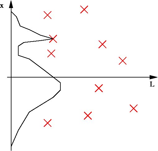 Figure 1
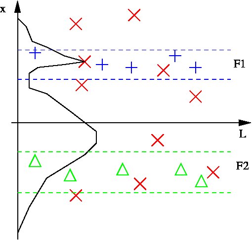 Figure 2
Peer Reviews
No public reviews on file for this paper yet. If you reviewed it on a platform where reviews are public (OpenReview, ICLR, NeurIPS, ICML), you can paste yours below so the community can read it here.
Videos
No videos yet. Explain this paper in a talk, walkthrough, or lecture? Add one.
Taxonomy
TopicsStochastic processes and statistical mechanics · Markov Chains and Monte Carlo Methods · Opinion Dynamics and Social Influence
Time-Homogeneous Diffusions with a Given Marginal at a
Random Time††thanks: Dedicated to Marc Yor on the occasion of his birthday.
Alexander Cox
Dept. of Mathematical Sciences
University of Bath
Bath BA2 7AY e-mail: [email protected]; web: www.maths.bath.ac.uk/$\sim$mapamgc/
David Hobson
Department of Statistics
University of Warwick
Coventry CV4 7AL e-mail: [email protected]; web: www.warwick.ac.uk/go/dhobson/
Jan Obłój
Mathematical Institute and
Oxford–Man Institute of Quantitative Finance
University of Oxford
Oxford OX1 3LB e-mail: [email protected]; web: www.maths.ox.ac.uk/$\sim$obloj/
Abstract
We solve explicitly the following problem: for a given probability measure , we specify a generalised martingale diffusion which, stopped at an independent exponential time , is distributed according to . The process is specified via its speed measure . We present three proofs. First we show how the result can be derived from the solution of Bertoin and Le Jan (1992) to the Skorokhod embedding problem. Secondly, we give a proof exploiting applications of Krein’s spectral theory of strings to the study of linear diffusions. Finally, we present a novel direct probabilistic proof based on a coupling argument.
1 Introduction
We are interested in the following general problem: suppose is a given distribution on , and suppose is a (possibly random) time. Find a time-homogeneous martingale diffusion, , independent of , for which is distributed according to . In particular, when is regular enough, we want to specify a function such that
[TABLE]
where is a Brownian motion. The process is a diffusion on natural scale described by its speed measure . When is less regular, the interpretation of as a speed measure remains valid, but may no longer have a density. In this case becomes a generalised or gap diffusion.
In this paper we present a solution to the problem in the case where is distributed exponentially with parameter 1. Somewhat surprisingly, not only does this problem always have a solution but also the solution is fully explicit. This can be seen both using a probabilistic and an analytic approach. More precisely, in Section 3 we exploit the general solution to the Skorokhod embedding problem of Bertoin and Le Jan (1992). This construction is essentially based on the theory of additive functionals for (nice) Markov processes. Then, in Section 4, we present a second proof based on the theory of generalised diffusions as presented in Kotani and Watanabe (1982). This is a more analytic approach which hinges on duality between generalised diffusions and strings and uses Krein’s spectral theory of strings.
Both of the above proofs exploit deep known results. In the final section, we present a direct proof from first principles. First we prove that the problem has a solution. We do this by writing as a time-changed Brownian motion, and hence is a solution to the Skorokhod embedding in : that is, has distribution . Our proof relies on a specific coupling of time-changes for different processes . Furthermore, the interpretation in terms of stopping times for gives an intuitive justification for the explicit formula for (i.e. in (1)).
1.1 Motivation
Our original goal was to solve the problem for the case where the time is a fixed, positive constant. Then, a time-homogeneous diffusion with marginal is in some sense the canonical, and perhaps simplest, process consistent with a given (single) marginal. For the problem with fixed and under sufficient smoothness conditions Jiang and Tao (2001) have proposed a relaxation scheme for calculating the diffusion co-efficient. However, to the best of our knowledge, existence and uniqueness for the problem with a general measure remain open. One application of this result would be to mathematical finance: the traded prices of call options with maturity can be used to infer the marginal distribution of the underlying asset under the pricing measure — note also that the price process , suitably discounted, is a martingale under this measure — so that the solution of the problem for fixed would give a canonical candidate price process consistent with market data. Other time-inhomogeneous processes exist with the correct time marginals (cf. Dupire (1994), Carr and Madan (1998), Madan and Yor (2002)), and the problem of finding examples, is related to the Skorokhod embedding problem. For further discussion of the Skorokhod embedding problem, and the connection to finance and model-independent hedging of derivatives, see Obłój (2004) or Hobson (2009).
Applications of the problem with exponentially distributed are discussed in a recent paper of Carr (2008). Carr proposes modelling the stock price process as a time-homogeneous diffusion time-changed by an independent gamma subordinator: . The clock is normalised so that has an exponential distribution, where is now the maturity of options whose prices are known, so that Carr (2008) effectively considers the same problem as the present paper. His approach is to use forward-backward Kolmogorov equations combined with Laplace transform properties. He is able to derive explicitly in (1), although he only considers with positive density and does not prove general existence or uniqueness results.
2 Generalised (gap) diffusions
We recall the classical construction of a generalised diffusion. Let be non-decreasing and right-continuous with and , . Assume further that . Then are well defined measures and we can define a measure on by
[TABLE]
where is the image of under . Naturally, can be defined directly from and we write and .
Consider a one-dimensional Brownian motion defined on , with , -a.s. We assume is rich enough to support random variables independent of . Let be the jointly continuous version of the local time of . We adopt here the classical Itô–McKean normalisation in which is a martingale. Put and let be the right-continuous inverse of . Then
[TABLE]
is a time-change of a Brownian motion and hence a strong Markov process living on . It is called a generalised diffusion (on natural scale) corresponding to the measure . It has also been called a gap diffusion in Knight (1981). Note that, due to our normalisation, the local time is twice the local time in Kotani and Watanabe (1982). In consequence is a generalised diffusion corresponding to measure in the notation of Kotani and Watanabe (1982). As an example, in this paper Brownian motion is a diffusion with speed measure equal to the Lebesgue measure and not twice the Lebesgue measure as in Kotani and Watanabe (1982).
In order to understand better the relationship between features of and the behaviour of we discuss two important classes, firstly where has a positive density, and secondly where only charges points.
Suppose first that for any . Then is a regular111i.e. for all , where . diffusion on with absorbing boundary points. is on natural scale and is simply its speed measure. We have and the measure can be recovered from as
[TABLE]
since it can be shown that is convex and, for , as measures on , see (Rogers and Williams, 2000, Sec. V.47) for a detailed discussion. If further , with bounded and uniformly positive on , then solves
[TABLE]
for a Brownian motion . Equivalently the infinitesimal generator of , when acting on functions supported on , is . Note that then and it can be verified directly from the occupation time formula that :
[TABLE]
From the above discussion we see that the regions where has more mass correspond to the regions where moves more slowly (and thus spends more time).
By a natural extension of the above analysis, if has zero mass in an interval, then since lives on the support of , this interval is not visited by at all. Conversely, if (and for every neighbourhood of , charges ), then is a sticky point for : started in , spends a positive time in even though it exits instantaneously.
It remains now to understand the role of isolated atoms in . Consider for , and . Then is a continuous-time Markov chain living on , stopped upon hitting or . From the construction it follows that can only jump to nearest neighbours, i.e. from it can jump to , and the probabilities of these follow instantly from the fact that is a martingale. The time spent in , , before jumps to a next point, has an exponential distribution with mean
[TABLE]
where is the first hitting time of for . (This is an example of the more general formula (for )
[TABLE]
for expected values of Brownian local times.) This completes the description of . We see that an isolated atom in has an effect of introducing a holding time in that point for , with mean proportional to .
3 Main result and probabilistic proof
Having recalled generalised diffusions we can now state the main result of our paper. In this section we provide a proof rooted in probabilistic arguments while in the next section we describe a more analytical approach. For a probability measure we let and denote respectively the lower and the upper bounds of its support.
Theorem 3.1**.**
Let be a probability measure, , and let . Define a measure by
[TABLE]
Let be the generalised diffusion associated with and be an –measurable –exponential random variable independent of . Then, under , and is a uniformly integrable martingale.
Proof.
It suffices to prove the theorem for as the general case follows by a simple shift in space. Assume in first instance that . Consider the following process : it takes values in , with added as an isolated point. starts in which is a holding point with parameter . On exit from at time , the process behaves as under the measure , so that , until exit from when jumps back to . In this way is a recurrent strong Markov process with as its regular starting point. Write for the probability measure associated with the process started at , noting that for all , the path jumps from to [math]. We make explicit the Bertoin and Le Jan (1992) solution to the Skorokhod embedding problem of in .
Let . The process admits a family of local times . We simply have , and for . This last quantity is exponentially distributed and independent of . It follows from (6) that
[TABLE]
The invariant measure for , displayed in in Bertoin and Le Jan (1992), acts by
[TABLE]
Consider a finite positive measure on and a positive continuous additive functional . The Revuz measure of is then given by
[TABLE]
so that and iff . We proceed to compute and , as defined in Bertoin and Le Jan (1992). We have and . Then, for ,
[TABLE]
and it follows that
[TABLE]
Jensen’s inequality grants us and hence is bounded as required. Furthermore, from (11), for
[TABLE]
since has support in . Hence the bound is best possible.
We have
[TABLE]
and the Bertoin and Le Jan (1992) stopping time is given by
[TABLE]
where . The key result of Bertoin and Le Jan (1992) is that solves the Skorokhod embedding problem for : i.e. . Recall that with the right–continuous inverse of , where is as displayed in (7). By the Corollary in (Bertoin and Le Jan, 1992, p. 540), from which it follows that . This allows us to rewrite as
[TABLE]
Hence , with an exponential random variable, as required. Note that by construction remains within the bounds of the support of . In particular, uniform integrability of follows from the fact that it is a bounded martingale.
Now consider an arbitrary and defined via (7). Note that and . Naturally if has a bounded support then the previous reasoning applies, so suppose that . For , let be the measure on , centred in zero and with on , and . Note that this defines and uniquely, converge to the bounds of the support of as , on , and converges weakly to , see Chacon (1977) for details. Let be the inverse of , with given by (7) for , and . Fix an exponential random variable independent of . By the construction above (applied with , so that the support of is contained in ), . Observe that, since on , we have for . Since , both and converge to the same limit in distribution as , and hence .
To see that the process is uniformly integrable, we note that this is equivalent to the process being uniformly integrable. This is easy to see as a consequence of Proposition 18 of Cox (2008), noting that since our laws are centered, uniform integrability and minimality are equivalent.
Finally, when only one of is infinite, say , the procedure is analogous but we only truncate the support of on one side, i.e. we look at on .
∎
4 An analytic proof
In the previous section, we proved Theorem 3.1 using a probabilistic approach, characteristic of the work of Bertoin and Le Jan (1992)). However, study of generalised diffusions can be seen as a probabilistic counterpart of the theory of strings, see Dym and McKean (1976). Indeed the theory of strings and original results in Kreĭn (1952) have played an important rôle in the study of fine properties of generalised diffusions including the Lévy measures of their inverse local times222Essentially Krein’s theorem provides a bijection between the set of strings and the set of their spectral measures. This is equivalent with a bijection between generalised diffusions with , reflected in zero, with the set of subordinators given by the inverse of the local time in zero of ., lower bounds on the spectrum of their infinitesimal generator, asymptotics of their transition densities and first hitting times distributions see Kac and Kreĭn (1958); Knight (1981); Kotani and Watanabe (1982); Küchler and Salminen (1989). It would be thus natural to re-derive (7) using analytic methods. This is indeed possible and we sketch here the main steps of such derivation.
Let be a generalised diffusion associated with a measure as in (2). Recall that in the notation of Kotani and Watanabe (1982) is associated to measure . Let and be defined as in (3.1)–(3.4) in Kotani and Watanabe (1982) (but with our normalisation of ):
[TABLE]
These functions yield a direct representation (3.5) therein:
[TABLE]
of the resolvent density , defined by
[TABLE]
for continuous bounded functions on the support of .
In what follows we take and drop the argument. We have and it can be checked independently (or deduced from (14)–(15) above) that are non-negative with non-increasing, and non-decreasing. Further we have as and as . This is described in detail, in the case of standard diffusion processes, in Theorem 5.13.3 in Itô (2006) (note that our is the solution therein), see also (Kotani and Watanabe, 1982, p. 241) and (Knight, 1981, p. 57). Furthermore, from their definitions, we have
[TABLE]
Assume for simplicity that is a centred probability measure: , and put . Then, Theorem 3.1 is simply equivalent to showing that for and given by (7), that is , we have .
Observe now that also solves (16) and as . Given that solves (14) it follows that for some constant . It remains to show that . For this we analyse the derivative in zero. On the one hand we have
[TABLE]
and on the other hand
[TABLE]
from which it follows that as required.
To end this section we check that the boundary behaviour of at is what we would expect it to be. Consider for example . If then we have
[TABLE]
In a similar manner we have
[TABLE]
Hence, by definition, is a natural boundary for which can not be reached in finite time starting from a point , see (Itô, 2006, Sections 5.11 and 5.16).
Suppose . First note that is a trap since by the definition of in (7), and hence is absorbed in upon reaching it. Further we have
[TABLE]
It follows that if is the endpoint of a regular interval for , i.e. if for all then is a regular or exit boundary and hence the process can reach in finite time. Finally, if is an isolated point in the support of , i.e. if for some , then likewise it is an isolated absorbing point in the state space of . It is easy to see that it can be reached in finite time with positive probability by considering reaching the point and behaving thereafter.
5 A more intuitive and direct proof
We have so far presented two methods of arriving at the representation (7) and Theorem 3.1. Both relied on deep probabilistic or analytic results and neither method appears to give a strong insight into why the result might be true. Consequently, one might want to have a more bare-handed proof, particularly if one wishes to generalise the result to other settings. Our goal in this section, is to give a direct proof of Theorem 3.1, using a coupling and a construction of a martingale diffusion as a time-change of Brownian motion. The intuitive picture on which we base our proofs exploits the fact that we can write a time-changed martingale diffusion as a Brownian motion. In this picture, ‘locally’, the process would appear to stop according to an exponential random variable, whose parameter would depend on the speed of the diffusion at that location; generalising this idea, we propose modelling the choice of an exponential stopping time by a Poisson Random measure on , where points are placed with intensity , i.e. with more frequency in places where we expect to stop more often. Then we stop the process at a point , if there is a point at in the Poisson random measure, and if the local time of the Brownian motion at reaches , before the local time at any other reaches for some other point of the Poisson random measure. By comparing these stopping times derived from different Poisson random measures, we are able to prove a monotonicity result. This gives us a coupling argument from which we deduce the existence of a measure with the desired stopping distribution, i.e. . Some simple calculations show that construction of a suitable generalised diffusion follows. This new insight then allows us to give an intuitive justification of the explicit formula (7). Observe that effectively we re-interpret the original problem as a new problem of finding a solution to the Skorokhod embedding problem (cf. Obłój (2004)) in a given class of stopping times .
We fix the underlying Brownian motion and the stopping times will be based on its local times . We think about the behaviour of the process in the context of the curve of the local times of as is increasing. More specifically, define
[TABLE]
which is the set of points ‘inside’ the local time curve. Now, given a measure , we suppose is a Poisson Random Measure on with intensity measure , independent of the Brownian motion . We allow to be infinite on some intervals. More precisely we assume that there exists a, possibly infinite, interval , containing the origin, such that for any compact set and that . This agrees with (2). Formally the measure decomposes into where is a Poisson Random measure with intensity and . We adopt this convention from now on.
We define the stopping time
[TABLE]
Figure 1 shows a graphical representation of the construction.
The idea now is to construct such that and then time change with to obtain the desired generalised diffusion process as in (3). This is explained in the following theorem.
Theorem 5.1**.**
*Given a centered probability distribution on there exists a measure such that is minimal333Following Monroe (1972), a stopping time is minimal if a.s. and imply a.s.. Then if is a centred random variable, and , minimality of is equivalent to the uniform integrability of . and embeds : .
Furthermore, if is a generalised diffusion given via (3) then the stopping time*
[TABLE]
is exponentially distributed, independently of , and .
Remark 5.2**.**
The above statement has two advantages in our opinion. Firstly, it provides an additional insight into the relation between stopping times for and . Secondly, it can be proved using a fairly direct and elementary arguments. We note however that it is poorer than Theorem 3.1 which not only gives existence of but also the explicit formula (7).
Proof.
We prove the first part of the theorem in two steps: in Step 1 we assume that has bounded support and in Step 2 we extend the result to arbitrary via a limiting proceedure. Finally we prove the second part of the theorem.
Whenever no ambiguity is possible we suppress the superscripts .
Part I: Step 1. We assume that has bounded support and denote by the smallest closed interval with . Define the set
[TABLE]
We will now show that this set has non-trivial elements. Fix and let on and infinity elsewhere. We have then , where , and thus . Let and define:
[TABLE]
Then we deduce:
[TABLE]
In consequence, for , . We want to take the maximal element of and the following lemma describes the key property for our proof.
Lemma 5.3**.**
Suppose that . Then the measure444See the proof of Lemma 5.3 for a detailed definition of . is also an element of .
The proof of the Lemma, perhaps the most interesting element of the proof of Theorem 3.1, is postponed. Using the Lemma we can conclude that there exists a maximal element . We claim that . Suppose the contrary and let . As is an element of , is dominated by on and with our assumption there exists such that . Let be the Radon-Nikodym derivative of with respect to on . Then there exists an and such that on and . Let with and let . The measure involves extra stopping in , when compared with , so that necessarily there is less chance in stopping off . Hence, on . Moreover, using arguments as above we see that on and thus which contradicts maximality of . Finally, is minimal since it is smaller than .
Part I: Step 2. Consider any centered probability measure and write respectively for the lower and the upper bound of the support of . We have just treated the case when both are finite so we suppose that at least one of them is infinite. Let be two sequences with , , as , such that the measure
[TABLE]
is centered. This measure can be embedded using where is the maximal element of . Clearly for all and thus is a decreasing sequence. It thus converges to a limit denoted , which is a measure (see e.g. Sec. III.10 in Doob (1994)).
Let and , , be independent Poisson measures with intensities respectively and , . Consider which is again a Poisson point measure with intensity . With as previously, we have that . Furthermore, as we have that so that as . To show that a.s. we recall that is a martingale. As we have that
[TABLE]
The left hand side converges to which is thus finite and in particular a.s. Finally, since for all , the law of is dominated by on and is thus simply equal to . The uniform integrability of follows from standard arguments (e.g. Proposition 18 of Cox (2008)).
Part II. To show that is exponentially distributed, we recall the above definitions. Then for :
[TABLE]
where for the last equality we use the fact that local times are continuous in . However, conditional on , we know is Poisson with parameter
[TABLE]
where we used (5). Clearly . Finally a similar calculation to the ones above shows that and is independent of . This completes the proof of Theorem 5.1. ∎
Proof of Lemma 5.3.
Note that the measure is well defined. More precisely let and and the Radon-Nikodym derivatives respectively of and with respect to . The measure is defined via its Radon-Nikodym derivative with respect to . Likewise, the measure is well defined. We write for the law of . Note that by construction and hence .
Consider the signed measure and let be the support of its positive part and the support of its negative part. Then we may decompose associated with into three independent Poisson Random Measures, with intensity , with intensity and with intensity . We know that the stopping times generated by the measures and both lead to measures which are dominated by on . We wish to deduce the same about .
We show this by considering the coupling implied by Figure 2. Given a set , we need to show that . However by considering , it is clear that since adding adding extra marks according to can only reduce the probability of stopping in , as it will not produce any new ‘points’ in this set. Similarly, for , we will have . Finally, for we have . It now follows from that . ∎
We have thus proved existence of a suitable measure such that the generalised diffusion associated to satisfies for an independent exponential time . We have also seen that this is equivalent to finding such that , where is stopping time defined in (20). We can use this new interpretation to recover the formula (7) for . Indeed, from construction of , intuitively we have
[TABLE]
The time spent in by is simply and . Hence, if we are to have we have to have
[TABLE]
which is exactly (7).
The reference list from the paper itself. Each links out to its DOI / PubMed record.
- 1Bertoin and Le Jan (1992) Bertoin, J., Le Jan, Y., 1992. Representation of measures by balayage from a regular recurrent point. Ann. Probab. 20 (1), 538–548.
- 2Carr (2008) Carr, P., 2008. Local variance gamma, unpublished, private communication.
- 3Carr and Madan (1998) Carr, P., Madan, D., 1998. Determining volatility surfaces and option values from an implied volatility smile. In: Avellaneda, M. (Ed.), Quantitative Analysis of Financial Markets. Vol. II. pp. 163–191.
- 4Chacon (1977) Chacon, R. V., 1977. Potential processes. Trans. Amer. Math. Soc. 226, 39–58.
- 5Cox (2008) Cox, A. M. G., 2008. Extending Chacon-Walsh: minimality and generalised starting distributions. In: Séminaire de probabilités XLI. Vol. 1934 of Lecture Notes in Math. Springer, Berlin, pp. 233–264.
- 6Doob (1994) Doob, J. L., 1994. Measure theory. Vol. 143 of Graduate Texts in Mathematics. Springer-Verlag, New York.
- 7Dupire (1994) Dupire, B., 1994. Pricing with a smile. Risk 7, 18–20.
- 8Dym and Mc Kean (1976) Dym, H., Mc Kean, H. P., 1976. Gaussian processes, function theory, and the inverse spectral problem. Academic Press [Harcourt Brace Jovanovich Publishers], New York, probability and Mathematical Statistics, Vol. 31.