
TL;DR
This paper explores the relationship between the Jones polynomial of knots and geometric properties of their complements, introducing invariants called Jones slopes and Jones period, and verifying conjectures through computations on various knot classes.
Contribution
It introduces the Jones slopes and Jones period invariants for knots, formulates related conjectures, and verifies them for specific classes of knots, advancing understanding of knot invariants and geometry.
Findings
Jones slopes form a finite set of rational numbers.
Conjectures hold for alternating and torus knots.
Explicit computations support the proposed relations.
Abstract
The paper introduces Slope Conjecture which relates the degree of the Jones polynomial of a knot and its parallels with the slopes of incompressible surfaces in the knot complement. More precisely, we introduce two knot invariants, the Jones slopes (a finite set of rational numbers) and the Jones period (a natural number) of a knot in 3-space. We formulate a number of conjectures for these invariants and verify them by explicit computations for the class of alternating knots, torus knots, the knots with at most 9 crossings, and the pretzel knots.
Click any figure to enlarge with its caption.
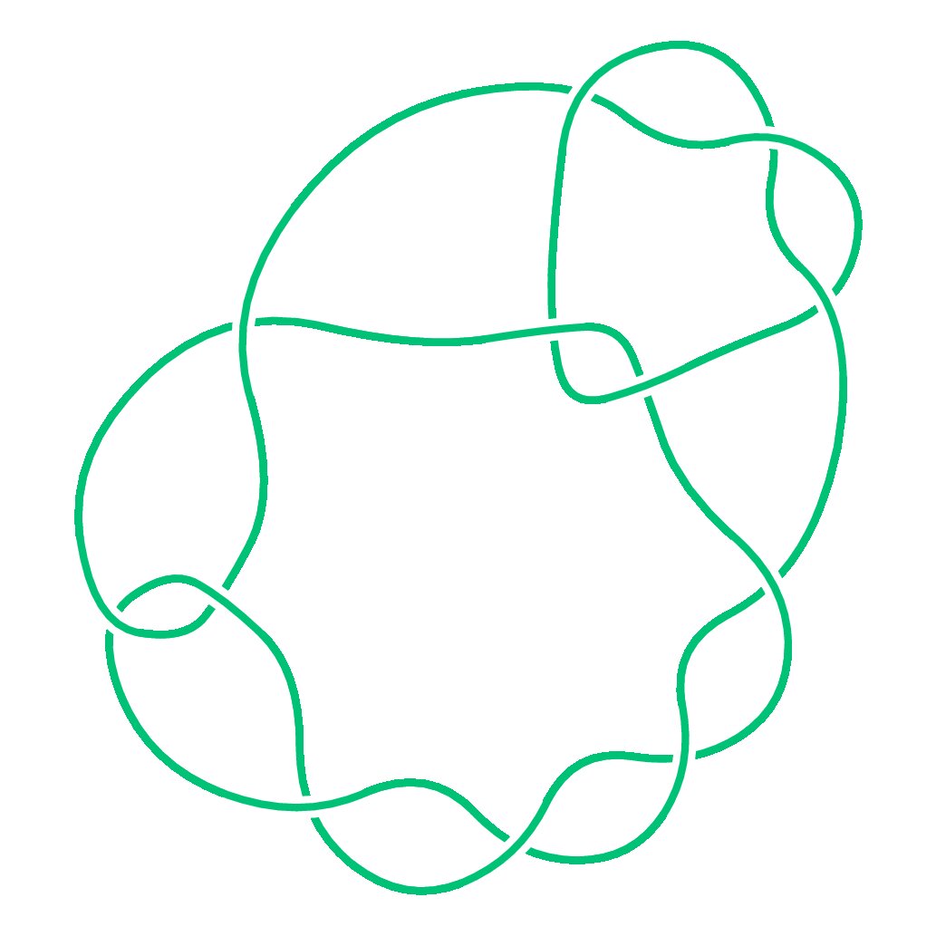 Figure 1
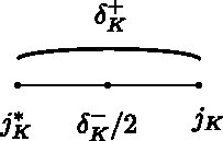 Figure 2
Peer Reviews
No public reviews on file for this paper yet. If you reviewed it on a platform where reviews are public (OpenReview, ICLR, NeurIPS, ICML), you can paste yours below so the community can read it here.
Videos
No videos yet. Explain this paper in a talk, walkthrough, or lecture? Add one.
The Jones slopes of a knot
Stavros Garoufalidis
School of Mathematics
Georgia Institute of Technology
Atlanta, GA 30332-0160, USA
.edu/stavros
(Date: May 21, 2010)
Abstract.
The paper introduces the Slope Conjecture which relates the degree of the Jones polynomial of a knot and its parallels with the slopes of incompressible surfaces in the knot complement. More precisely, we introduce two knot invariants, the Jones slopes (a finite set of rational numbers) and the Jones period (a natural number) of a knot in 3-space. We formulate a number of conjectures for these invariants and verify them by explicit computations for the class of alternating knots, the knots with at most 9 crossings, the torus knots and the pretzel knots.
The author was supported in part by NSF.
1991 Mathematics Classification. Primary 57N10. Secondary 57M25.
*Key words and phrases: Knot, link, Jones polynomial, Jones slope, Jones period, quasi-polynomial, alternating knots, signature, pretzel knots, polytopes, Newton polygon, incompressible surfaces, slope, Slope Conjecture. *
Contents
-
1.1 The degree of the Jones polynomial and incompressible surfaces
-
1.2 The degree of the colored Jones function is a quadratic quasi-polynomial
-
1.5 The symmetrized Jones slopes and the signature of a knot
-
3 The Jones slopes and the Jones period of an alternating knot
1. Introduction
1.1. The degree of the Jones polynomial and incompressible
surfaces
The paper introduces an explicit conjecture relating the degree of the Jones polynomial of a knot (and its parallels) with slopes of incompressible surfaces in the knot complement. We give an elementary proof of our conjecture for alternating knots and torus knots, and check it with explicit computations for non-alternating knots with and crossings, and for the pretzel knots.
One side of our conjecture involves the growth rate of the degree (with respect to ) of the colored Jones function of a knot. The other side involves the finite set of slopes of incompressible, -incompressible orientable surfaces in the complement of , where the slopes are normalized so that the longitude has slope [math] and the meridian has slope ; [Ha]. To formulate our conjecture, we need a definition. Recall that is a cluster point of a sequence of real numbers if for every there are infinitely many indices such that . Let denote the set of cluster points of a sequence .
Definition 1.1**.**
(a) For a knot , define the Jones slopes by:
[TABLE]
(b) Let denote the set of boundary slopes of incompressible surfaces of .
A priori, the structure and the cardinality of the set is not obvious. On the other hand, it is known that is a finite subset of ; see [Ha]. Normal surfaces are of special interest because of their relation with exceptional Dehn surgery, and the character variety and hyperbolic geometry, see for example [Bu, CGLS, CCGLS, KR, LTi, Mv].
Conjecture 1**.**
(The Slope Conjecture) For every knot we have
[TABLE]
Before we proceed further, and to get a better intuition about this conjecture, let us give three illustrative examples.
Example 1.2*.*
For the alternating knot we have:
[TABLE]
where and are the maximum and the the minimum degree of with respect to . On the other hand, according to [Cu], the Newton polygon (based on the geometric component of the character variety) has sides and its slopes (excluding multiplicities) are
[TABLE]
The reader may observe that and are quadratic polynomials in and four times the leading terms of and are boundary slopes (namely and ), and moreover they agree with and where is the number of positive/negative crossings of . In addition, as Y. Kabaya observed (see [Ka]), has slopes outside the interval .
Example 1.3*.*
For the non-alternating pretzel knot we have:
[TABLE]
where is a periodic sequence of period given by if respectively. is a Montesinos knot and its boundary slopes are given by
[TABLE]
(see [HO] and [Du] and compare also with [Ma]). In this case, is no longer a quadratic polynomial of . Instead is a quadratic quasi-polynomial with fixed leading term . Moreover, four times this leading term is a slope of the knot. This number was the motivating example that eventually lead to the results of this paper. Likewise, four times the -coefficient of is [math], which is also a boundary slope of this knot.
Example 1.4*.*
The pretzel knots and are mutant, alternating and Montesinos. Since they are mutant, their colored Jones functions (thus their Jones slopes) agree; see [Kf]. Since they are alternating, their common Jones slopes are and ; see Theorem 2. Since they are Montesinos, Hatcher-Oertel’s algorithm implemented by Dunfield (see [Du]) implies that their boundary slopes are given by
[TABLE]
It follows that the set is not invariant under knot mutation.
1.2. The degree of the colored Jones function is a quadratic
quasi-polynomial
In the previous section, we took the shortest path to formulate a conjecture relating the degree of the colored Jones function of a knot with incompressible surfaces in the knot complement. In this section we will motivate our conjecture, and add some structure to it. Let us recall that in 1985, Jones introduced the famous Jones polynomial of a knot (or link) in 3-space; [Jo]. The Jones polynomial of a knot is a Laurent polynomial with integer coefficients that tightly encodes information about the topology and the geometry of the knot.
Unlike the Alexander polynomial, not much is known about the topological meaning of the coefficients of the Jones polynomial, nor about its degree, nor about the countable set of Jones polynomials of knots.
This unstructured behavior of the Jones polynomial becomes more structured when one fixes a knot and considers a stronger invariant, namely the colored Jones function . The latter is a sequence of elements of indexed by which encodes the TQFT invariants of a knot colored by the irreducible -dimensional representation of , and normalized to be at the unknot; see [Tu2]. With these conventions, and is the Jones polynomial of .
In many ways, the sequence is better behaved, and suitable limits of the sequence have a clear topological or geometric meaning. Let us give three instances of this phenomenon:
- (a)
A suitable formal power series limit (known as the Melvin-Morton-Rozansky Conjecture) equals to and determines the Alexander polynomial of (see [B-NG]).
- (b)
An analytic limit for small complex numbers near zero equals to also determines the Alexander polynomial of ; see [GL1, Thm.2].
- (c)
The exponential growth rate of the sequence (the so-called Kashaev invariant) of a hyperbolic knot is conjectured to equal to the volume of , divided by ; see [Ks].
On the other hand, one can easily construct hyperbolic knots with equal Jones polynomial but different Alexander polynomial and volume.
Some already observed structure regarding the colored Jones function is that it is -holonomic, i.e., it satisfies a linear recursion relation with coefficients in ; see [GL1]. The present paper is concerned with another notion of regularity, namely the degree of the colored Jones function with respect to . Since little is known about the degree of the Jones polynomial of a knot, one might expect that there is little to say about the degree of the colored Jones function . Once observed, the regularity of the degree seems obvious as Bar-Natan suggests; see [B-NL, Lem.3.6] and [Me]. Moreover, the degree of the colored Jones function motivates the introduction of two knot invariants, the Jones slopes of a knot (a finite set of rational numbers) and the Jones period of a knot (a natural number).
1.3. -holonomic functions and quadratic quasi-polynomials
To formulate our new notion of regularity, we need to recall what is a quasi-polynomial. A quasi-polynomial is a function
[TABLE]
for some where is a periodic fuction with integral period for ; [St, BR]. If is not identically zero, then the degree of is . We will focus on two numerical invariants of a quasi-polynomial, its period and its slopes.
Definition 1.5**.**
(a) The period of a quasi-polynomial as above is the common period of .
(b) The set of slopes of a quadratic quasi-polynomial is the finite set of twice the rational values of the periodic function .
Notice that if is a quasi-polynomial of period , then there exist polynomials such that when , and vice-versa. Notice also that the set of slopes of a quasi-polynomial is always a finite subset of .
Quasi-polynomials of period are simply polynomials. Quasi-polynomials appear naturally in counting problems of lattice points in rational convex polytopes; see for example [BP, BR, BV, Eh, St]. In fact, if is a rational convex polytope, then the number of lattice points of is the so-called Ehrhart quasi-polynomial of , useful in many enumerative questions [BP, BR, BV, Eh, St].
The next theorem seems obvious, once observed. The proof, given in [Ga2], uses ideas from differential Galois theory of -modules and the key Skolem-Mahler-Lech theorem from number theory. Let denote the degree of a rational function with respect to .
Theorem 1**.**
[Ga2]** If is a -holonomic sequence of rational functions, then for large , is a quadratic quasi-polynomial. Moreover, the leading term of satisfies a linear recursion relation with constant coefficients.
The restriction for large in Theorem 1 is necessary, since the sequence is -holonomic, and its degree (given by if , by if is even and by if is odd) is not a quasi-polynomial. On the other hand, if , the degree is given by the quadratic quasi-polynomial .
Corollary 1.6**.**
If is a -holonomic sequence of rational functions and then
[TABLE]
Proof.
Consider a subsequence of the natural numbers such that
[TABLE]
Since is (for large ) given by a quasi-polynomial, it follows that for a periodic function and for all . Since takes finitely many values, it follows that there is a subsequence of such that for all , where is a slope of . Since for all , it follows that . I.e., is a slope of . Conversely, it is easy to see that every slope of is the limit point for a subsequence taken to be an arithmetic progression on which takes a constant value. ∎
1.4. The Jones slopes and the Jones period of a knot
Given a knot , we set
[TABLE]
Combining the -holonomicity of the colored Jones function of a knot with Theorem 1, it follows that is a quadratic quasi-polynomial for large .
Definition 1.7**.**
(a) The Jones period is the period of .
(b) The Jones slopes is the finite set of slopes of .
Corollary 1.6 implies that for every knot we have:
[TABLE]
where the right-hand side (and consequently, the left-hand side, too) is a finite subset of .
Lemma 1.8**.**
For every knot we have:
[TABLE]
where is a finite subset of .
The invariant records the growth rates of the (maximum) degree of the colored Jones function of . We can also record the minimum degree as follows. If denotes the mirror image of , then . Let us define
[TABLE]
Notice that Conjecture 1 applied to implies that
[TABLE]
The next proposition gives a bound for the Jones slopes of a knot in terms of the number of positive/negative crossings of a planar projection.
Proposition 1.9**.**
For every knot , every and every we have
[TABLE]
The reader may compare the above lemma with Example 1.2.
Our next theorem confirms Conjecture 1 for all alternating knots. Consider a reduced planar projection of with crossings of positive/negative sign.
Theorem 2**.**
If is alternating, then
[TABLE]
In addition, the two checkerboard surfaces of (doubled, if need, to make them orientable) are incompressible with slopes and .
Our final lemma relates the Jones slopes and the period of a knot.
Lemma 1.10**.**
If is an integer-valued quadratic quasi-polynomial with period , then for every slope of we have
[TABLE]
In particular, for every knot we have
[TABLE]
Thus, if a knot has a non-integral Jones slope, then it has period bigger than .
1.5. The symmetrized Jones slopes and the signature of a knot
In this section we discuss the symmetrized version of :
[TABLE]
Of course, and . Pictorially, we have:
[TABLE]
As we will see below, the symmetrized degree of the colored Jones function has a different flavor, and relates (at least for alternating knots) to the signature of the knot. is the span of , i.e., the difference between the maximum and minimum degree of . On the other hand, is the sum of the minimum and maximum degree of , and appears to be less studied. Of course, are quadratic quasi-polynomials. Since the colored Jones function is multiplicative under connected sum, and reverses to under mirror image, it follows that
[TABLE]
Our next theorem computes the quasi-polynomials of an alternating knot in terms of three basic invariants: the signature , the writhe and the number of crossings of a reduced projection of . Our result follows from elementary linear algebra using the results of Kauffman, Murasugi and Thistlethwaite, [Kf, Mu, Th], further simplified by Turaev [Tu1]. See also [Li, p.42] and [Le, Prop.2.1].
Theorem 3**.**
(a) For all alternating knots we have:
[TABLE]
(b) The Jones polynomial determines by:
[TABLE]
(c) The Jones polynomial of and its 2-parallel determines and by:
[TABLE]
Remark 1.11*.*
Part (c) of Theorem 3 is sharp. The Jones polynomial of an alternating knot determines the number of crossings, but it does not determine the signature nor the writhe of the knot. Shumakovitch provided us with a table of pairs of alternating knots with up to crossings (using the Thistlethwaite notation) with equal Jones polynomials and unequal signature. An example of such a pair is with crossings is the knot and its mirror image:
[TABLE]
has Jones polynomial
[TABLE]
and signature . Since the signature is nonzero, is not amphicheiral, and yet has palindromic Jones polynomial. The next colored Jones polynomial is given by:
[TABLE]
and it is far from being palindromic. This is another example where the pattern of the Jones polynomial is blurred, but the pattern of the colored Jones function is clearer.
Results similar to Theorem 2 and 3 have been also been obtained independently in [CT] using the Jones polynomial of an alternating knot.
Let us end this section with two comments. In this paper is a knot, but without additional effort one can state similar results for a link (and even a knotted trivalent graph, or quantum spin network) in 3-space. In addition, we should point out that there are deeper aspects of stability and integrality of the coefficients of the colored Jones function. We will discuss them in a future publication.
1.6. Plan of the proof
In Section 3 we use the Kauffman bracket skein module and the work of Kauffman, Le, Murasugi Thistlethwaite to give a proof of Proposition 1.9 and Theorems 2 and 3. This proves our Slope Conjecture for all alternating knots.
In Section 4 we give computational evidence for the degree of the colored Jones polynomials (and for the Slope Conjecture) of the non-alternating knots with and crossings. In addition, we verify the Slope Conjecture for all pretzel knots (using the fusion state-sum formulas of the colored Jones function studied in [GL3, Co, GVa]), and all torus knots (using Morton’s formula for the colored Jones function of those, [Mo]). The reader may note that the pretzel knots are well-known examples of Montesinos knots, with non-integral slopes (for ), which are not quasi-alternating, thus the results of [FKP] do not apply for this family.
2. Future directions
In this section we will discuss some future directions, and pose some questions, problems and conjectures.
The Slope Conjecture involves knots in 3-space, and relates the degree of the colored Jones function to their set of boundary slopes. The Slope Conjecture may be extended in three different directions: one may consider (a) links in 3-space, (b) general 1-cusped manifolds and (c) general Lie algebras. These extensions have been considered by the author. In [GVu] we introduce a Slope Conjecture for knots and arbitrary Lie algebras. One may also consider 1-cusped manifolds with the homology of , i.e., knot complements in integer homology spheres. For those, the colored Jones polynomial exists (though it is not a polynomial, but rather an element of the Habiro ring; see [GL2]). The colored Jones function is -holonomic, and we can use the non-commutative -polynomial of this sequence to define the set of slopes.
The following problem appears mysterious and tandalizing.
Problem 1**.**
Understand the Selection Principle which selects
- (a)
the Jones slope from the set of boundary slopes,
- (b)
the colored Jones function from the vector space of solutions of the linear -difference equation.
Now, let us post some questions, based on the limited experimental evidence. Our first question concerns the class of knots of Jones period .
Question 1**.**
Is it true that a prime knot is alternating if and only if ?
Theorem 2 proves the easy direction of the above conjecture. As a warm-up for our next question, several authors have studied the diameter of the set
[TABLE]
See for example [IM1, IM2, MMR]. Y. Kabaya pointed out to us that there are alternating knots with diameter bigger than twice the number of crossings; see Example 1.2. Let denote the Jones diameter
[TABLE]
Proposition 1.9 shows that . Moreover, the bound is achieved for alternating knots, and more generally for adequate knots; see [FKP]. The next question concerns the class of knots of maximal Jones diameter.
Question 2**.**
Is it true that a prime knot is adequate if and only if ?
The class of alternating knots is included in two natural classes: quasi-alternating knots, and adequate knots. Knot Homology (and its exact triangles) can tell whether a knot is quasi-alternating or not (see [OM]), but it seems hard to tell whether a knot is alternating or not. Adequate knots appeared in [LT] in relation to the Jones polynomial and also in [FKP]. It was pointed out to us by D. Futer, E. Kalfagianni J. Purcell and P. Ozsváth that the pretzel knots are not adequate nor quasi-alternating for .
In all examples, the set consists of a single element, whereas the set can have arbitrarily many elements. Thus, Conjecture 1 sees only a small part of the set . Our next conjecture claims that the colored Jones function of may see all the elements in . To formulate it, recall that is a -holonomic sequence, and satisfies a unique, minimal order recursion relation of the form
[TABLE]
where are polynomials with greatest common divisor ; see [Ga1]. The 3-variable polynomial is often called the non-commutative -polynomial of . The AJ Conjecture of [Ga1] states that every irreducible factor of is a factor of or is -free, and vice-versa. Here denotes the -polynomial of and contains all components of the character variety of (including the abelian one). Let denote the slopes of the Newton polygon of . These are the so-called visible slopes of a knot. It follows by Culler-Shalen theory (see [CS, CGLS, CCGLS]) that .
Let us define the -Newton polytope of to be the convex hull of the monomials of . is a convex polytope in , and we may consider the image of it in under the projection map which maps to (i.e., sends the monomial to ).
Definition 2.1**.**
The -slopes of a knot are the slopes of the projection of to .
Problem 2**.**
Show that for every knot we have
[TABLE]
It is easy to see that for every knot we have . In fact, this holds for arbitrary -holonomic sequences; see [Ga4, Prop.1.2] for a detailed discussion. Thus, Problem 2 implies Conjecture 1. The AJ Conjecture motivates Problem 2. This is discussed in detail in [Ga4].
Our next problem concerns the symmetrized quasi-polynomial of a knot from (7). Although is not a concordance invariant, it determines the signature of an alternating knot.
Problem 3**.**
Show that determines a Knot Homology invariant.
3. The Jones slopes and the Jones period of an alternating knot
In this Section we prove Proposition 1.9 and Theorems 2 and 3 for an alternating knot , using the Kauffman bracket presentation of the colored Jones polynomial.
The following lemma of Le [Le, Prop.2.1], (based on well-known properties of the Kauffman bracket skein module) shows that the sequences and have at most quadratic growth rate with respect to . More precisely, for every knot we have:
[TABLE]
This implies that the slopes of the quadratic quasi-polynomial satisfy . Replacing by its mirror , it implies the same inequality for the slopes of and concludes the proof of Proposition 1.9. ∎
Consider a reduced planar projection of an alternating knot with positive/negative crossings. Then, the number of crossings and the writhe of are given by and . Let denote the signature of . Then we can express the minimum and maximum degrees and of in terms of and . This was shown by Kauffman, Murasugi and Thistlethwaite, [Kf, Mu, Th], and further simplified by Turaev [Tu1]. See also [Li, p.42] and [Le, Prop.2.1]. With our conventions, Proposition 2.1 of [Le] states that for all we have:
[TABLE]
where (resp. ) is the number of circles of the (resp. ) smoothing of the planar projection. For example, for the right-handed trefoil , we have
[TABLE]
and
[TABLE]
[TABLE]
and
[TABLE]
Murasugi and Turaev observe that [Tu1, p.219-220]
[TABLE]
Equation (16) implies that is a quadratic polynomial (i.e., a quasi-polynomial of period ) with coefficient of equal to , i.e., with slope . This concludes the proof of Theorem 2. Equations (7), (16), (16) and (18) prove the first part of Theorem 3.
It remains to show that the two checkerboard surfaces of a reduced projection of an alternating knot have slopes and . Observe that if is the slope of a surface (where is the standard meridian-longitude pair) and denotes the form in the boundary of a neighborhood of , then , . If is a black surface with slope , then the geometrically and intersect at a point, thus . In addition, follows the knot as we move towards the crossing, and intersects twice around each positive crossing, and none around each negative crossing. The result follows. ∎
Remark 3.1*.*
Let denote the 3-dimensional -vector space spanned by the functions on the set of alternating knots. There is an involution on this set, which includes an involution on :
[TABLE]
On the other hand, , and belong to and
[TABLE]
Thus, is a -linear combination of , and is a -linear combination of and . This is precisely the content of Theorem 3.
Remark 3.2*.*
Let denote the coefficient of in a polynomial . Equations (9) and (10) imply that for all alternating knots we have:
[TABLE]
and
[TABLE]
4. Computing the Jones slopes and the Jones period of a knot
4.1. Some lemmas on quasi-polynomials
To better present the experimental (and in some cases, proven) data presented in the next section, let us give some lemmas on quasi-polynomials. If is a sequence of numbers, consider the generating series
[TABLE]
The next well-known lemma characterizes quasi-polynomials. appears in [St, Prop.4.4.1] and [BR, Lem.3.24].
Lemma 4.1**.**
[St, Prop.4.4.1]**[BR*, Lem.3.24]** The following are equivalent:
*(a) is a quasi-polynomial of period
(b) the generating series
[TABLE]
is a rational function where , every zero of satisfies (provided that has been reduced to lowest term) and .
(c) For all ,
[TABLE]
where each is a polynomial function of and each satisfies .
Moreover, the degree of in (22) is one less than the multiplicity of the root in , provided has been reduced to lowest terms.
Definition 4.2**.**
We say that a quadratic quasi-polynomial is mono-sloped if it has only one slope . In other words, we have
[TABLE]
where is a linear quasi-polynomial.
To phrase our next corollary, let denote the -th cyclotomic polynomial, and let denote Euler’s -function.
Corollary 4.3**.**
* is mono-sloped if and only if*
[TABLE]
where the summation is over a finite set of natural numbers and and has degree less than . Moreover,
[TABLE]
Proof.
Observe that
[TABLE]
if and only if
[TABLE]
∎
Proof.
(of Lemma 1.10) Given , there exists an arithmetic progression such that for all natural numbers we have
[TABLE]
Now, let
[TABLE]
Now, takes integer values at all integers. This implies that
[TABLE]
(see [BR]). The result follows. ∎
It is often easier to detect the periodicity properties of the the difference
[TABLE]
of a sequence . It is easy to recover from and .
Lemma 4.4**.**
With the above conventions, we have:
[TABLE]
Proof.
We have:
[TABLE]
∎
We can iterate the above by considering the -th difference defined by and for .
4.2. Computing the colored Jones function of a knot
There are several ways to compute the colored Jones function of a knot . For example, one may use a planar projection and -matrices; see for example, [Tu2, GL1] and also [B-N]). Alternatively, one may use planar projections and shadow formulas as discussed at length in [Co] and [GVa]. Or one may use fusion quantum spin networks and recoupling theory, discussed in [CFS, KL, Co, GVa]. All these approaches gives various useful formulas for presented as a finite sum of a proper -hypergeometric summand [GL1]. A careful inspection of the summand allows in several cases to compute the degree of .
4.3. Guessing the colored Jones function of a knot
In this section we guess the sequence of knots with a small number of crossings, using the following strategy, inspired by conversations with D. Zagier. Using the KnotAtlas [B-N] we compute as many values of the colored Jones function as we can, and record their degree. This gives us a table of values of the quadratic quasi-polynomials and . Taking the third difference of this table results into a degree [math] quasi-polynomial, i.e., a periodic function. At this point, we make a guess for this periodic function, and the corresponding generating series. Then, we use Lemma 4.4 and our guess for the second different to obtain a formula for and . The partial fraction decomposition then gives us a formula for and . In some cases, using explicit finite multi-dimensional sum formulas for the colored Jones polynomial, one can prove that the guessed formula for and are indeed correct. In this section, we will not bother with proofs.
As an example of our method, we will guess a formula for and for the pretzel knot. One can actually prove that our guess is correct, using the fusion formulas for the 3-pretzel knots, but we will not bother. The values of starting with are given by:
[TABLE]
Taking the first difference we get the following values of starting with :
[TABLE]
appears to be the constant sequence from which we guess that , and correspondingly the generating series is
[TABLE]
More interesting is the sequence starting with :
[TABLE]
Taking the first, second and third difference we obtain:
[TABLE]
Thus, we guess that is a periodic sequence with period and generating series
[TABLE]
Using Lemma 4.4 three times, we compute
[TABLE]
Taking the partial fraction decomposition, it follows that
[TABLE]
where is a periodic sequence of period given by:
[TABLE]
4.4. A summary of non-alternating knots
In this section we list the quasi-polynomials and of non-alternating knots with and crossings. In the Rolfsen table of knots, the non-alternating knots with crossings are where , with crossings are where . Let us give a combined table of the non-alternating knots with and crossings, their period , their Jones slopes and , and their distinct boundary slopes. The boundary slopes are computed using the program of [HO], corrected in [Du], which computes the boundary slopes of all Montesinos knots except which is not a Montesinos knots. In all those cases, the set of boundary slopes agrees with the slopes of the -polynomial of [Cu, CCGLS], once [math] is included.
[TABLE]
The above data are in agreement with Conjecture 1. Let us make a phenomenological remark regarding all examples of non-alternating knots with or crossings.
- (a)
and are mono-sloped, i.e., they are of the form where is a linear quasi-polynomial.
- (b)
For all knots, is a boundary slope, though not necessarily the largest one.
- (c)
In the case of the and knots, the degree of is and in all other cases, it is zero.
- (d)
The period of all non-alternating knots was greater than . knots have period , and has period . The period of for odd appears to be , and the number of crossings is . Thus the period can be asymptotically as large as the number of crossings.
- (e)
For the case of , the leading coefficient is and for it is .
4.5. The -crossing non-alternating knots
4.5.1. The knot
In the data below, we will give the first few values of and , the guessed decomposition of the generating series and of the quasi-polynomials and .
Some values of and starting with :
[TABLE]
[TABLE]
[TABLE]
where is a 2-periodic sequence. Note that in this example the values of for suffice to prove that is not a polynomial of .
4.5.2. The knot
[TABLE]
[TABLE]
[TABLE]
where is a linear quasi-polynomial with period .
4.5.3. The knot
[TABLE]
[TABLE]
[TABLE]
where is a 2-periodic sequence.
4.6. The -crossing non-alternating knots
4.6.1. The knot
[TABLE]
[TABLE]
[TABLE]
where is a 2-periodic sequence.
4.6.2. The knot
[TABLE]
[TABLE]
[TABLE]
where is a linear quasi-polynomial with period .
4.6.3. The knot
[TABLE]
[TABLE]
[TABLE]
where is a linear quasi-polynomial with period .
4.6.4. The knot
[TABLE]
[TABLE]
[TABLE]
where is a periodic sequence with period .
4.6.5. The knot
[TABLE]
[TABLE]
[TABLE]
where is a periodic sequence with period .
4.6.6. The knot
[TABLE]
[TABLE]
[TABLE]
where is a periodic sequence with period .
4.6.7. The knot
[TABLE]
[TABLE]
[TABLE]
where is a periodic sequence with period .
4.6.8. The knot
[TABLE]
[TABLE]
[TABLE]
where is a periodic sequence with period .
4.7. The case of the pretzel knots
A triple sum formula for the colored Jones polynomial of pretzel knots with 3 pretzels is available, and using it we can compute and for all pretzel knots of the form for odd ; see [GVa]. We will state the result of the computation here. Recall the -th difference of a sequence from Section 4.1. When is odd, we have:
[TABLE]
It follows that
[TABLE]
where are linear quasi-polynomials. When is odd we have:
[TABLE]
It follows that
[TABLE]
where are linear quasi-polynomials. Notice that the above formulas single out exceptional behavior at . The Jones period and the Jones slopes are given by
[TABLE]
On the other hand, Hatcher-Oertel and Dunfield (see [HO] and [Du]) compute the slopes of those Montesinos knots
[TABLE]
Compare also with Mattman [Ma, p.32] who computes which of those slopes are visible from the geometric component of the -polynomial. Equations (24) and (25) together with the fact that [math] is a boundary slope confirm Conjecture 1 for all pretzel knots.
4.8. The case of torus knots
In this section we will use Morton’s formula for the colored Jones function of a torus knot to compute the degree of the colored Jones function and verify Conjecture 1.
Let denote the torus knot for a pair of coprime integers . Since the mirror image of is , we will focus on the case of . With our conventions, Morton’s formula [Mo] for the colored Jones function is the following:
[TABLE]
For example,
[TABLE]
The summand of Equation (26) consists of two monomials with exponents quadratic functions of . A little calculation reveals that the maximum and minimum degree of the colored Jones function is given by
[TABLE]
Thus the period is when and when or . Since is alternating if and only if or , our results are in accordance to Question 1. The boundary slopes of are (see for example [HO]). This confirms Conjecture 1 for torus knots.
4.9. Acknowledgment
The author wishes to thank K. Ichihara, Y. Kabaya, T. Mattman, P. Ozsváth, A. Shumakovitch, R. van der Veen, D. Zagier, D. Zeilberger and especially M. Culler and N. Dunfield for numerous enlightening conversations. The idea of the Slope Conjecture was conceived during the New York Conference on Interactions between Hyperbolic Geometry, Quantum Topology and Number Theory in New York in the summer of 2009. The author wishes to thank the organizers, A. Champanerkar, O. Dasbach, E. Kalfagianni, I. Kofman, W. Neumann and N. Stoltzfus for their hospitality.
The reference list from the paper itself. Each links out to its DOI / PubMed record.
- 1[B-N] Bar-Natan, Knot Atlas , http://katlas.math.toronto.edu
- 2[B-NG] by same authorand S. Garoufalidis, On the Melvin-Morton-Rozansky conjecture , Inventiones, 125 (1996) 103–133.
- 3[B-NL] by same authorand R. Lawrence, A rational surgery formula for the LMO invariant , Israel J. Math. 140 (2004) 29–60.
- 4[BP] A. Barvinok and J.E. Pommersheim, An algorithmic theory of lattice points in polyhedra , New perspectives in algebraic combinatorics, Math. Sci. Res. Inst. Publ., 38 (1999) Cambridge Univ. Press 91–147.
- 5[BR] M. Beck and S. Robins, Computing the continuous discretely, Integer-point enumeration in polyhedra , Undergraduate Texts in Mathematics. Springer, (2007).
- 6[BV] M. Brion and M. Vergne, Lattice points in simple polytopes , J. Amer. Math. Soc. 10 (1997) 371–392.
- 7[Bu] B.A. Burton, Introducing Regina, the 3-manifold topology software , Experiment. Math. 13 (2004) 267–272.
- 8[CFS] S. Carter, D.E. Flath, M. Saito, The Classical and Quantum 6 j 6 𝑗 6j -symbols , Mathematical Notes 43, Princeton University Press, 1995.