A 3D radiative transfer framework: VI. PHOENIX/3D example applications
Peter H. Hauschildt, E. Baron

TL;DR
This paper demonstrates the application of a 3D radiative transfer framework within the PHOENIX/3D code, showcasing its scalability and accuracy across diverse atmospheric conditions for spectrum synthesis.
Contribution
It introduces an extended 3D version of PHOENIX, integrating the 3DRT framework, and validates its performance and accuracy against 1D models using various test cases.
Findings
3D radiative transfer calculations are feasible with current computational resources.
The 3D models show good agreement with 1D models in test cases.
The framework scales well with parallel computing.
Abstract
We demonstrate the application of our 3D radiative transfer framework in the model atmosphere code PHOENIX/3D for a number of spectrum synthesis calculations for very different conditions. The 3DRT framework discussed in the previous papers of this series was added to our general-purpose model atmosphere code PHOENIX/1D and an extended 3D version PHOENIX/3D was created. The \phxT code is parallelized via the MPI library using a hierarchical domain decomposition and displays very good strong scaling. We present the results of several test cases for widely different atmosphere conditions and compare the 3D calculations with equivalent 1D models to assess the internal accuracy of the 3D modeling. In addition, we show the results for a number of parameterized 3D structures. With presently available computational resources it is possible to solve the full 3D radiative transfer (including…
Click any figure to enlarge with its caption.
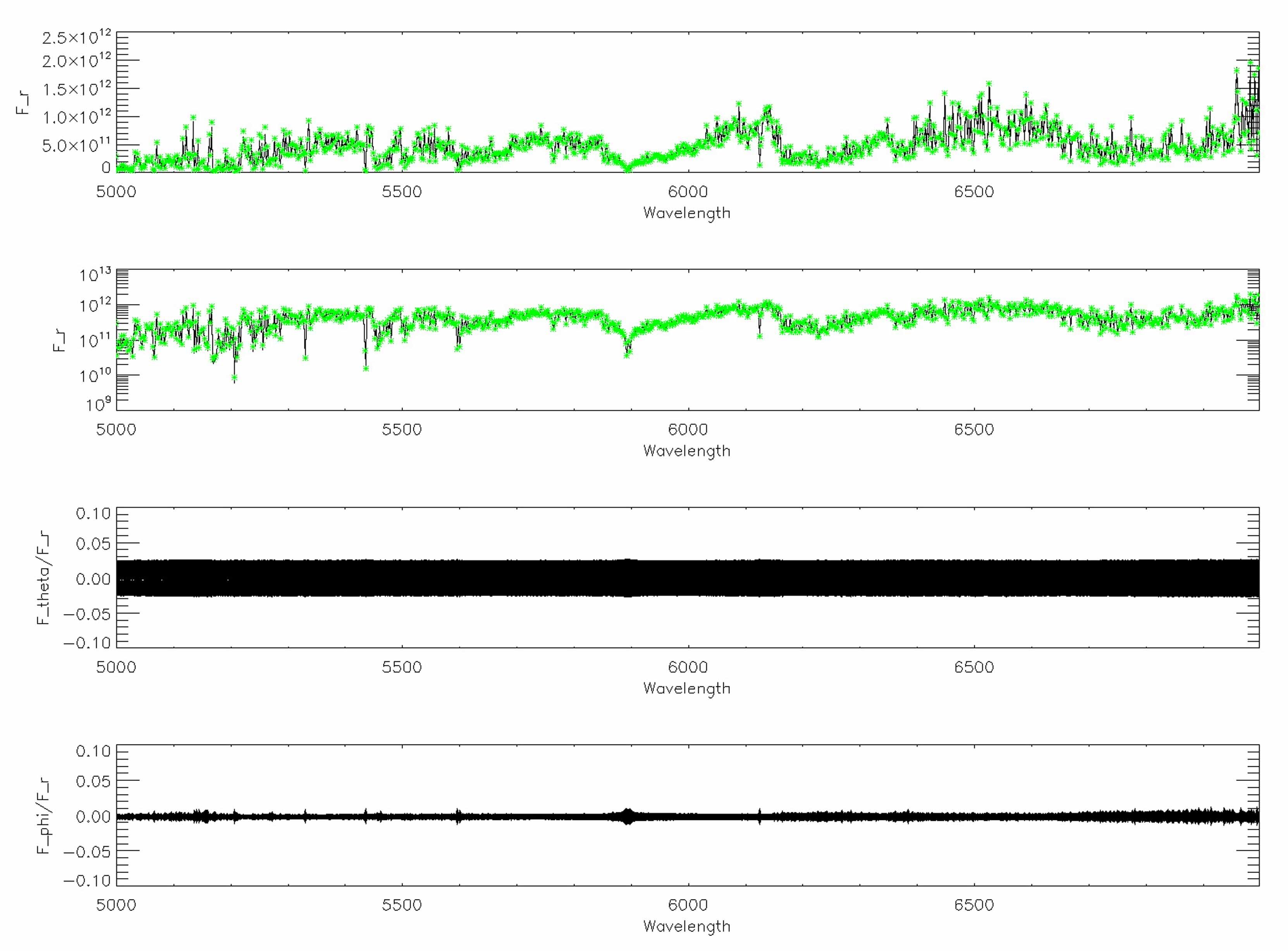 Figure 1
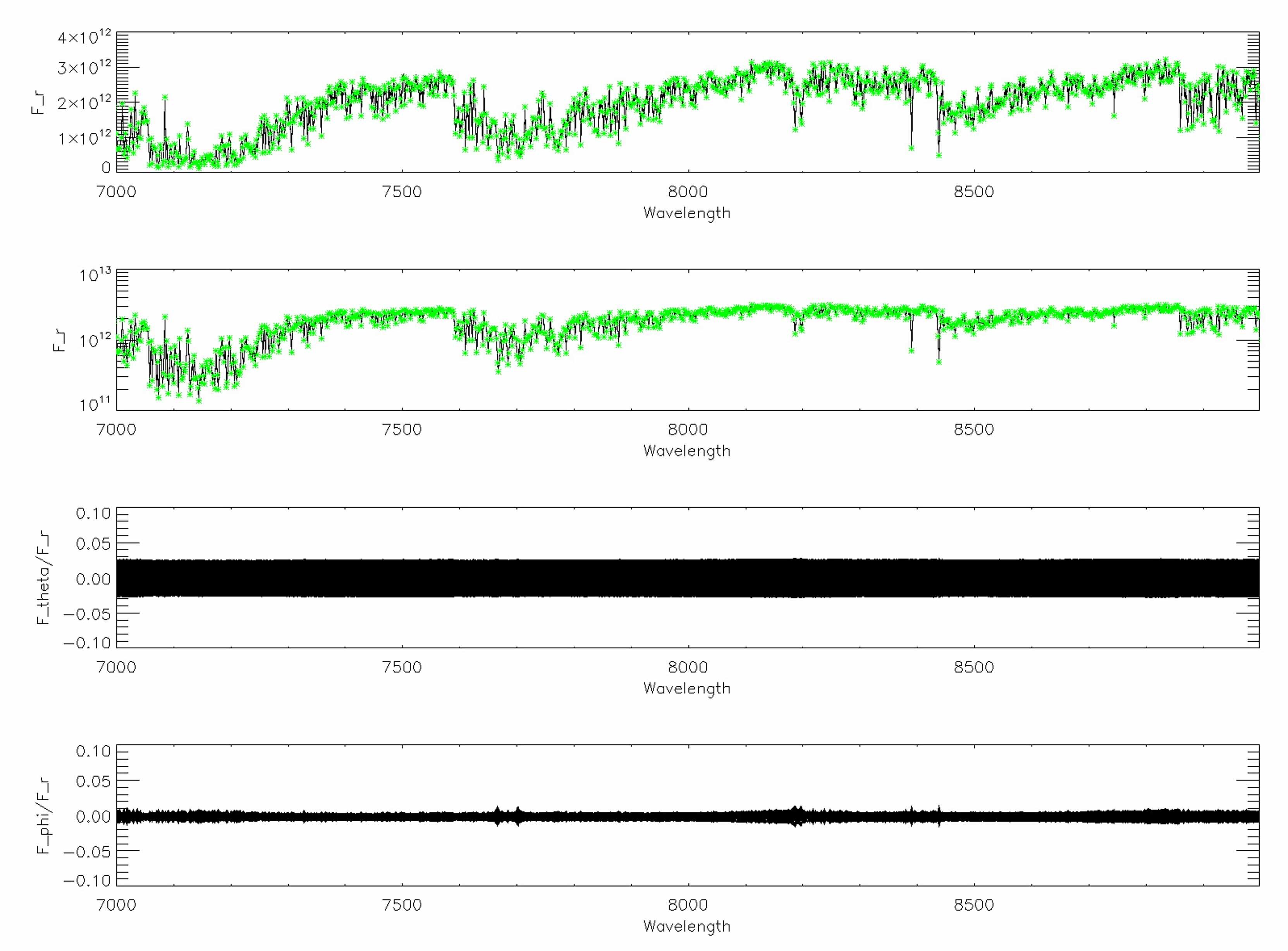 Figure 2
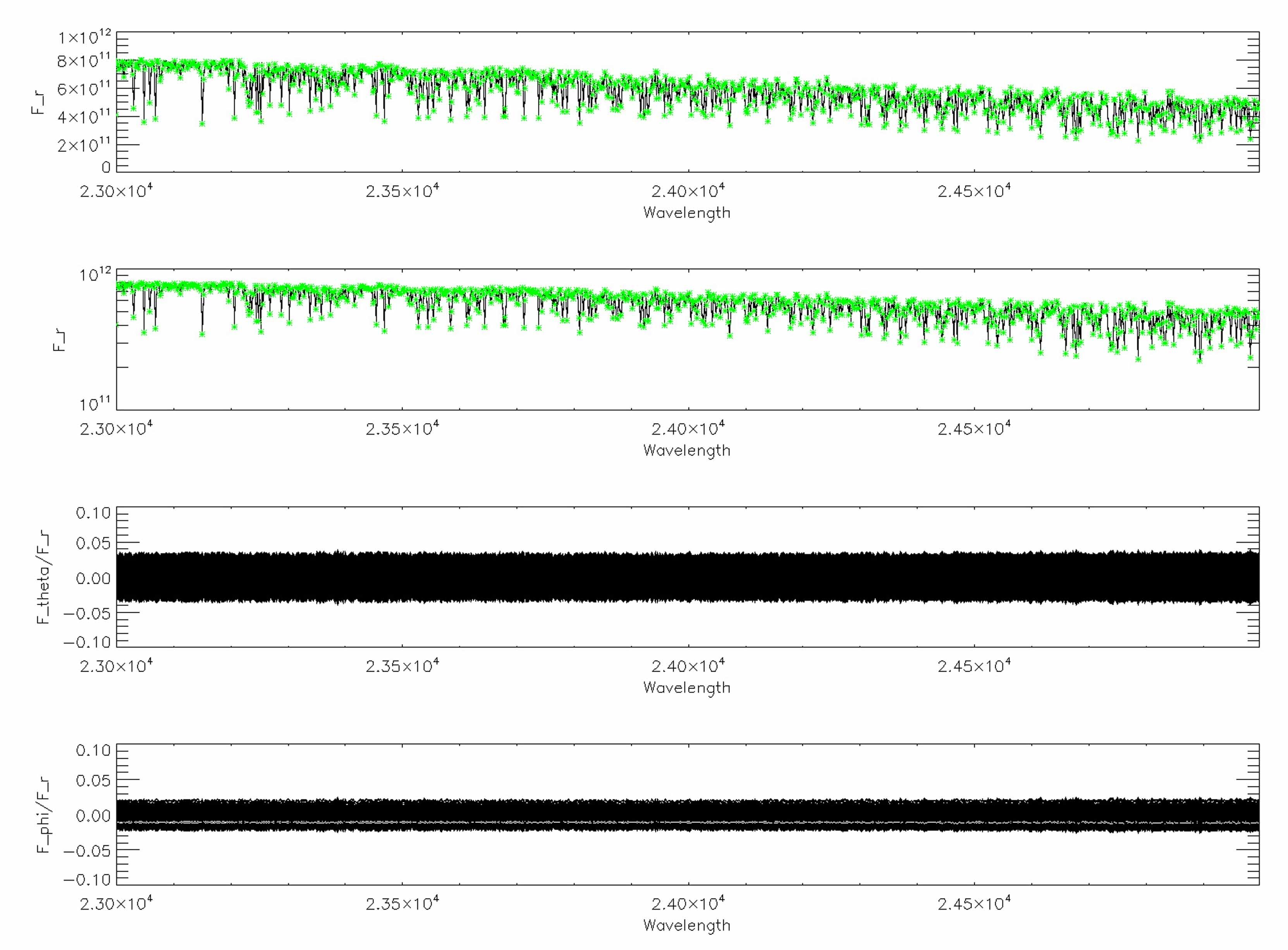 Figure 3
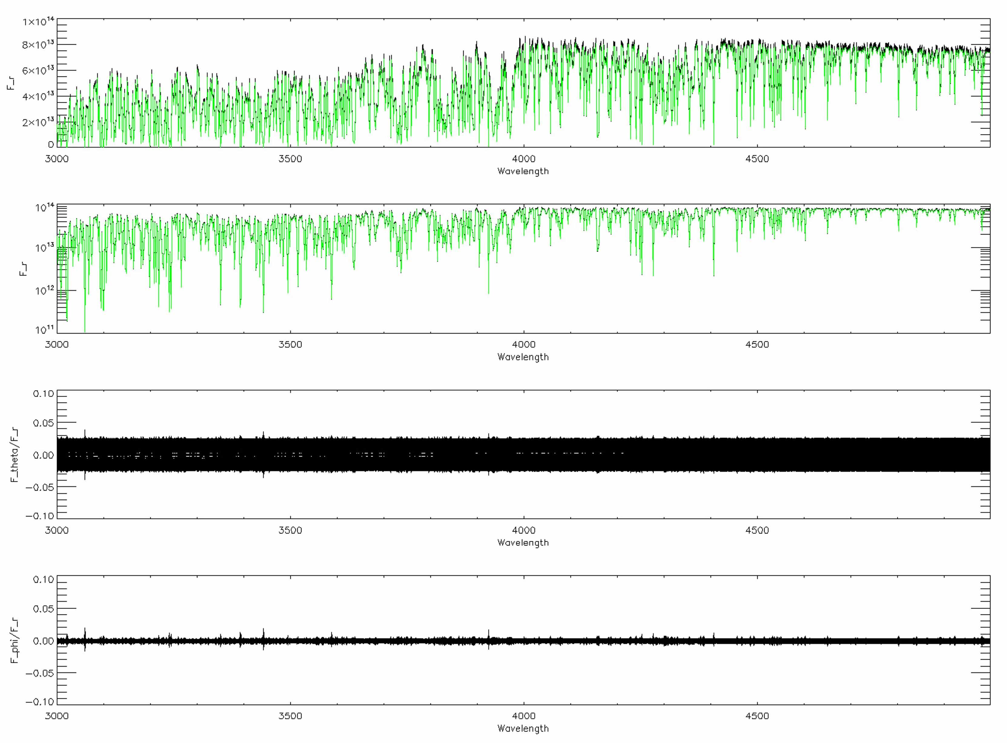 Figure 4
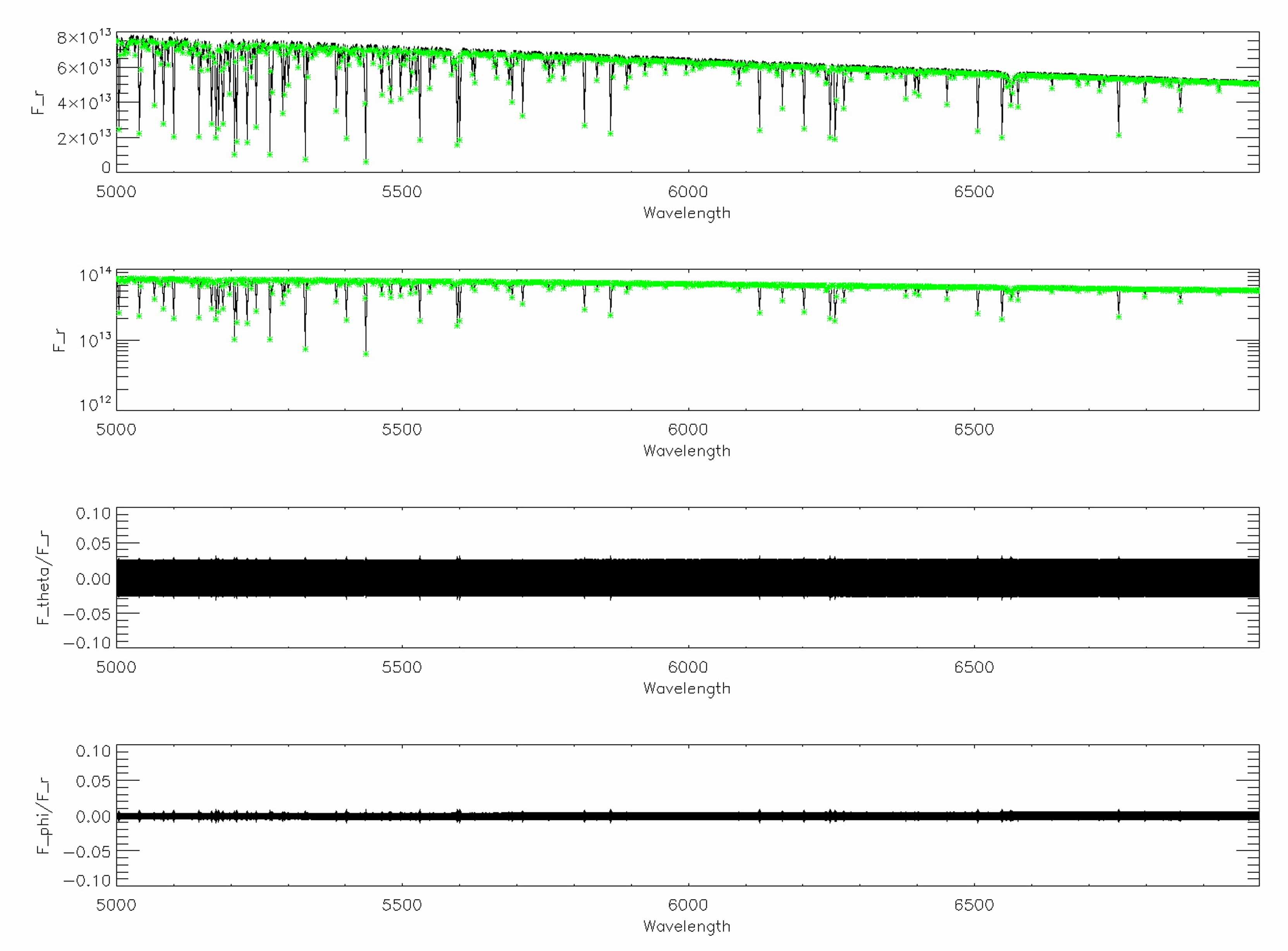 Figure 5
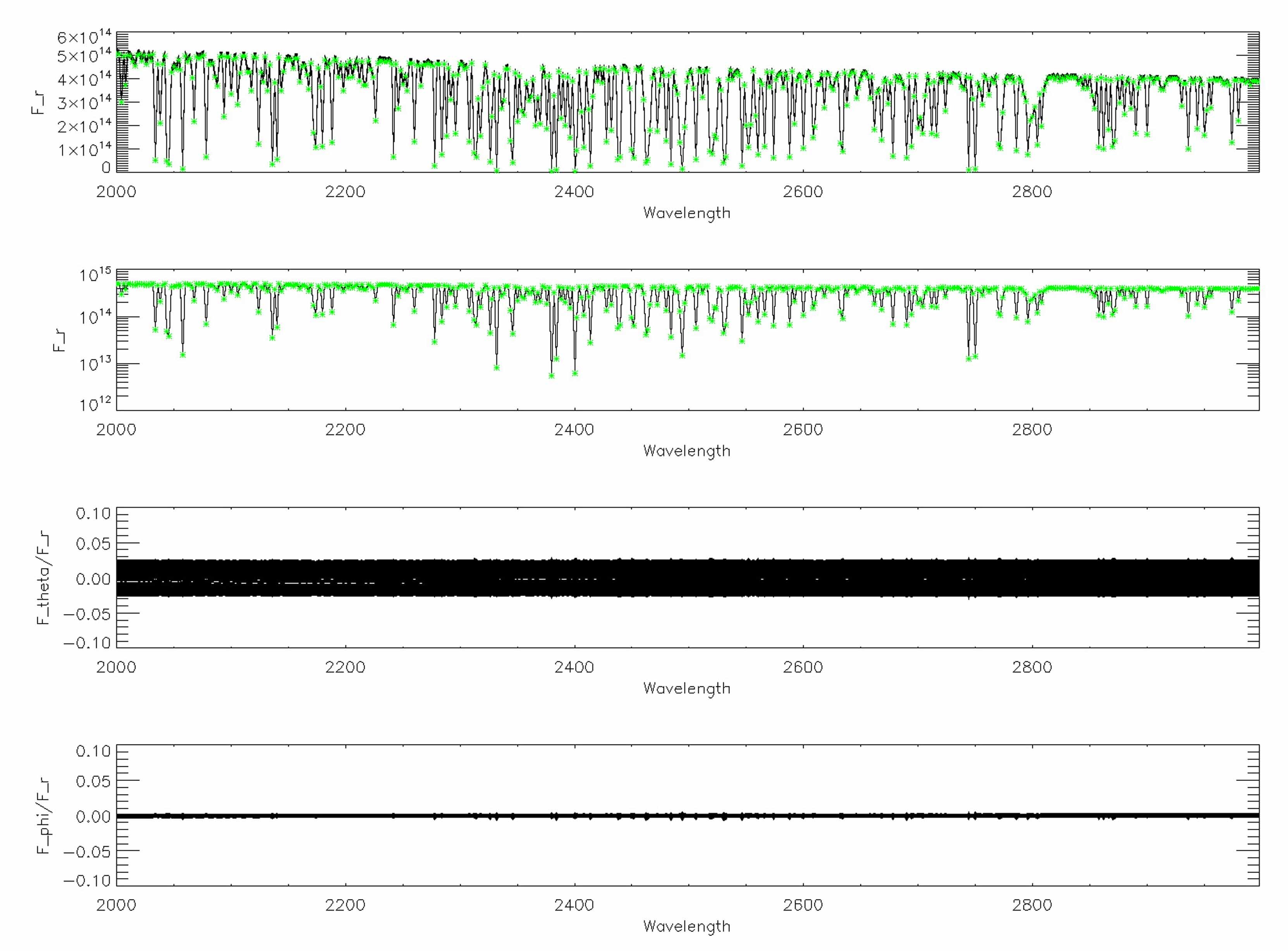 Figure 6
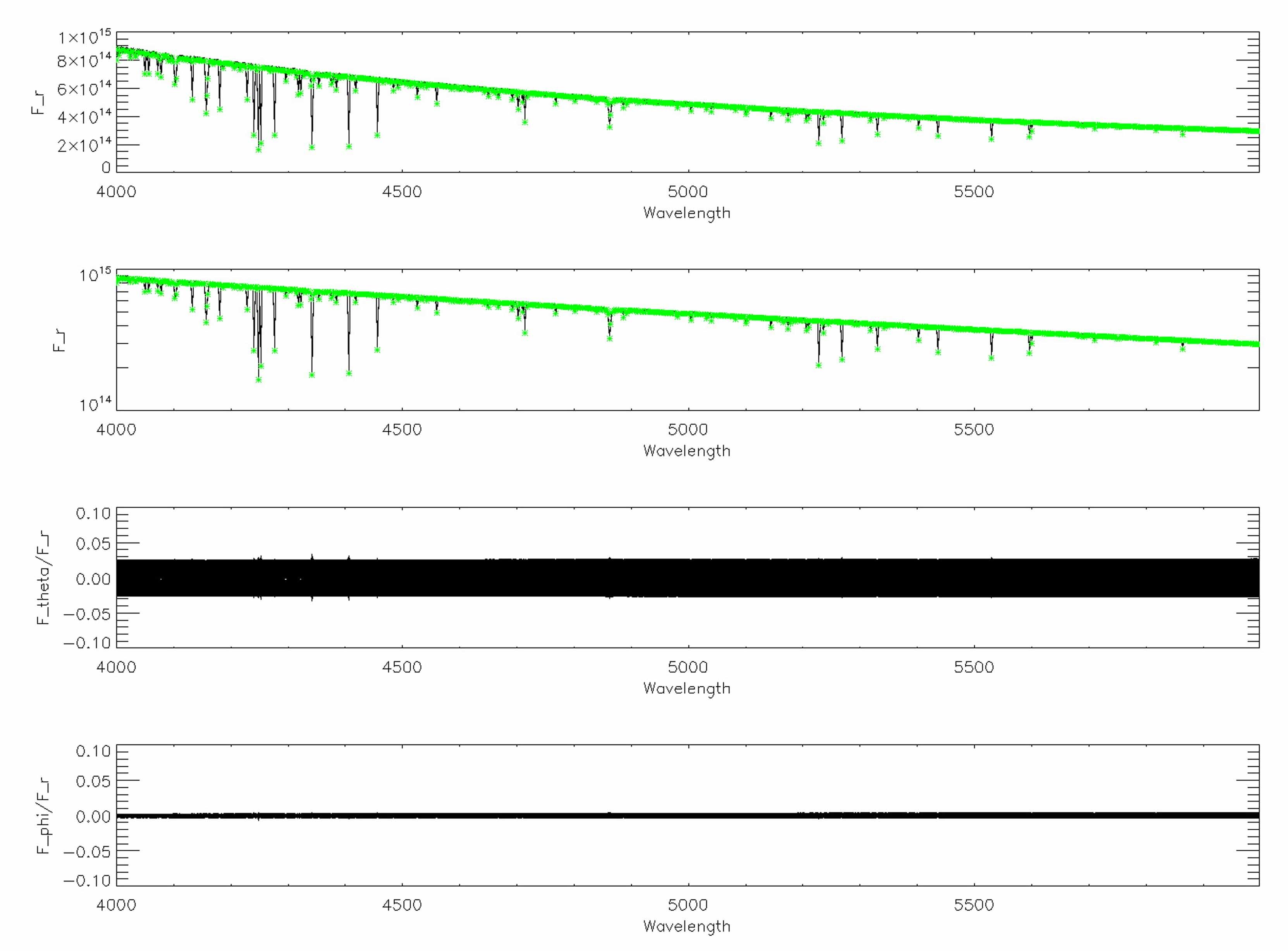 Figure 7
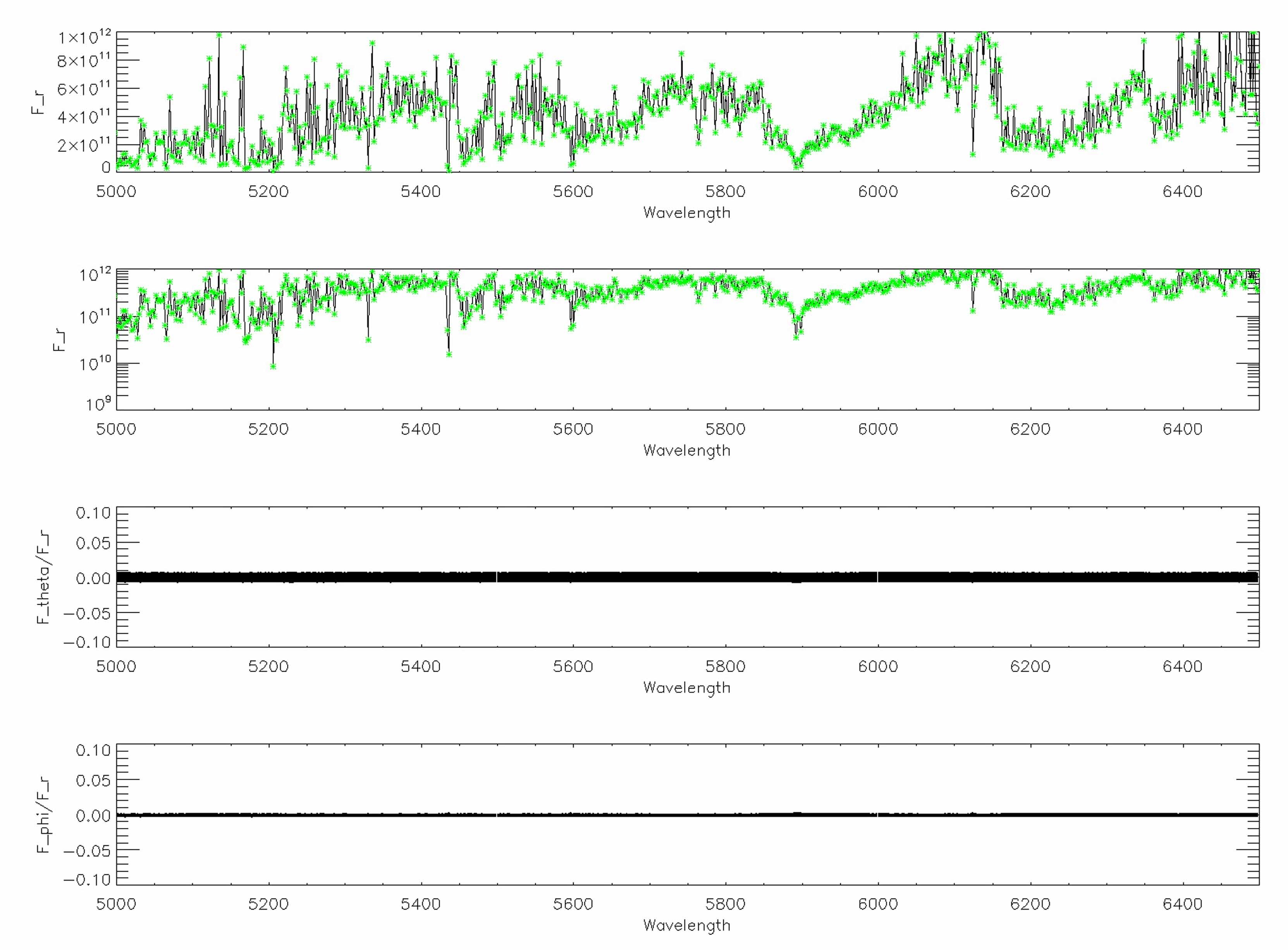 Figure 8
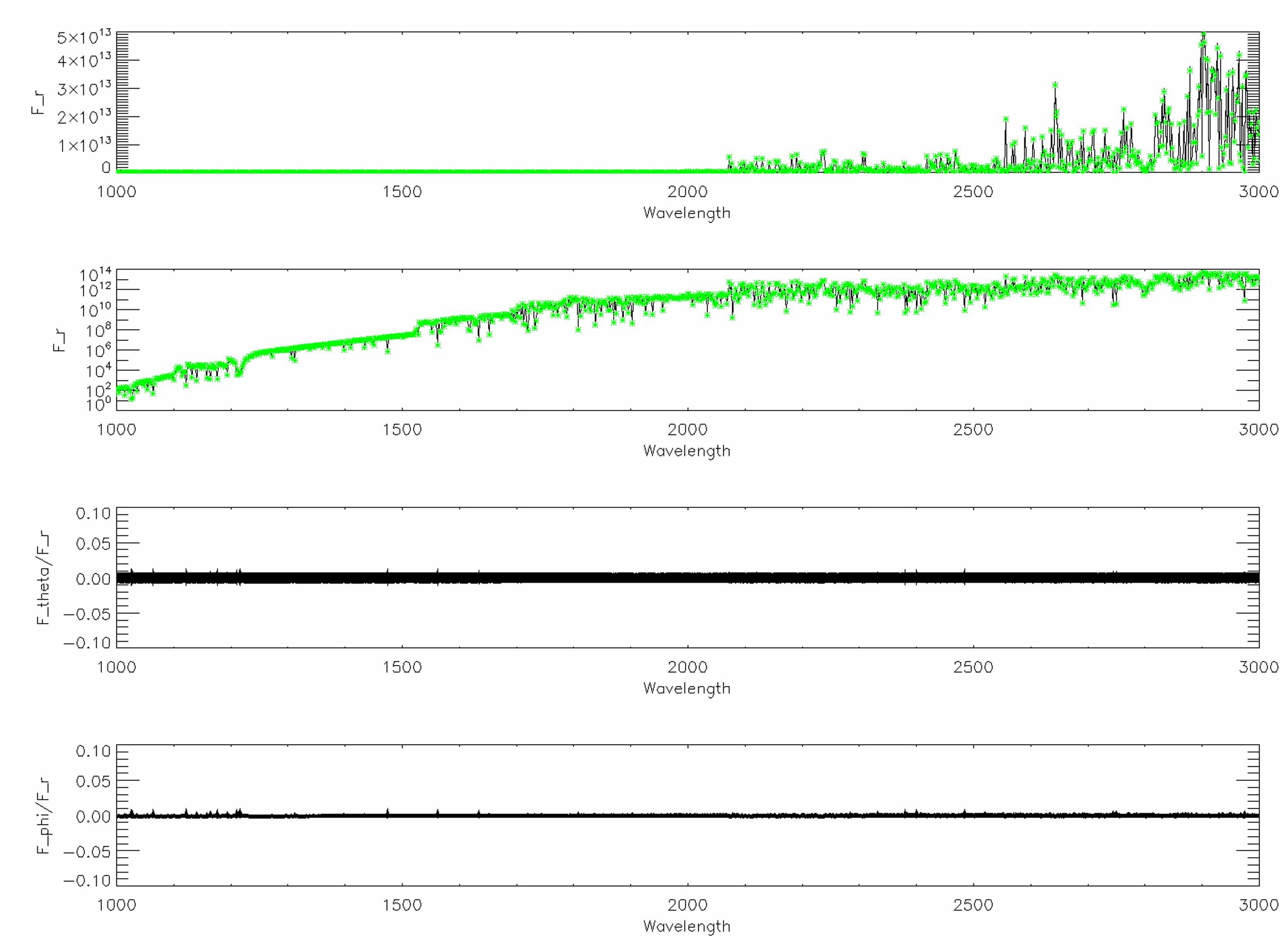 Figure 9
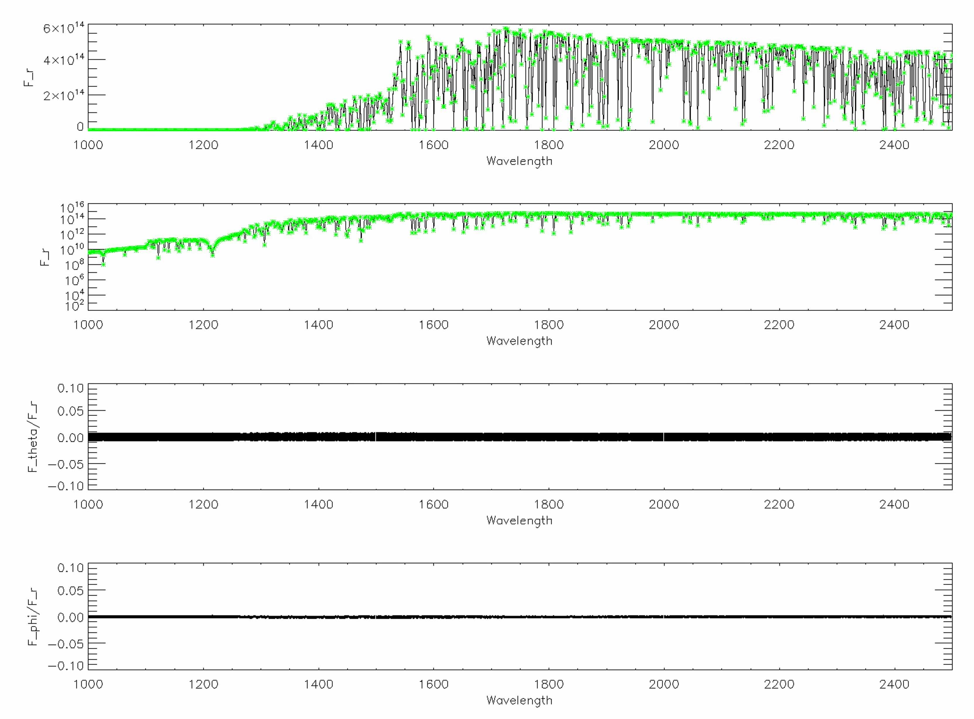 Figure 10
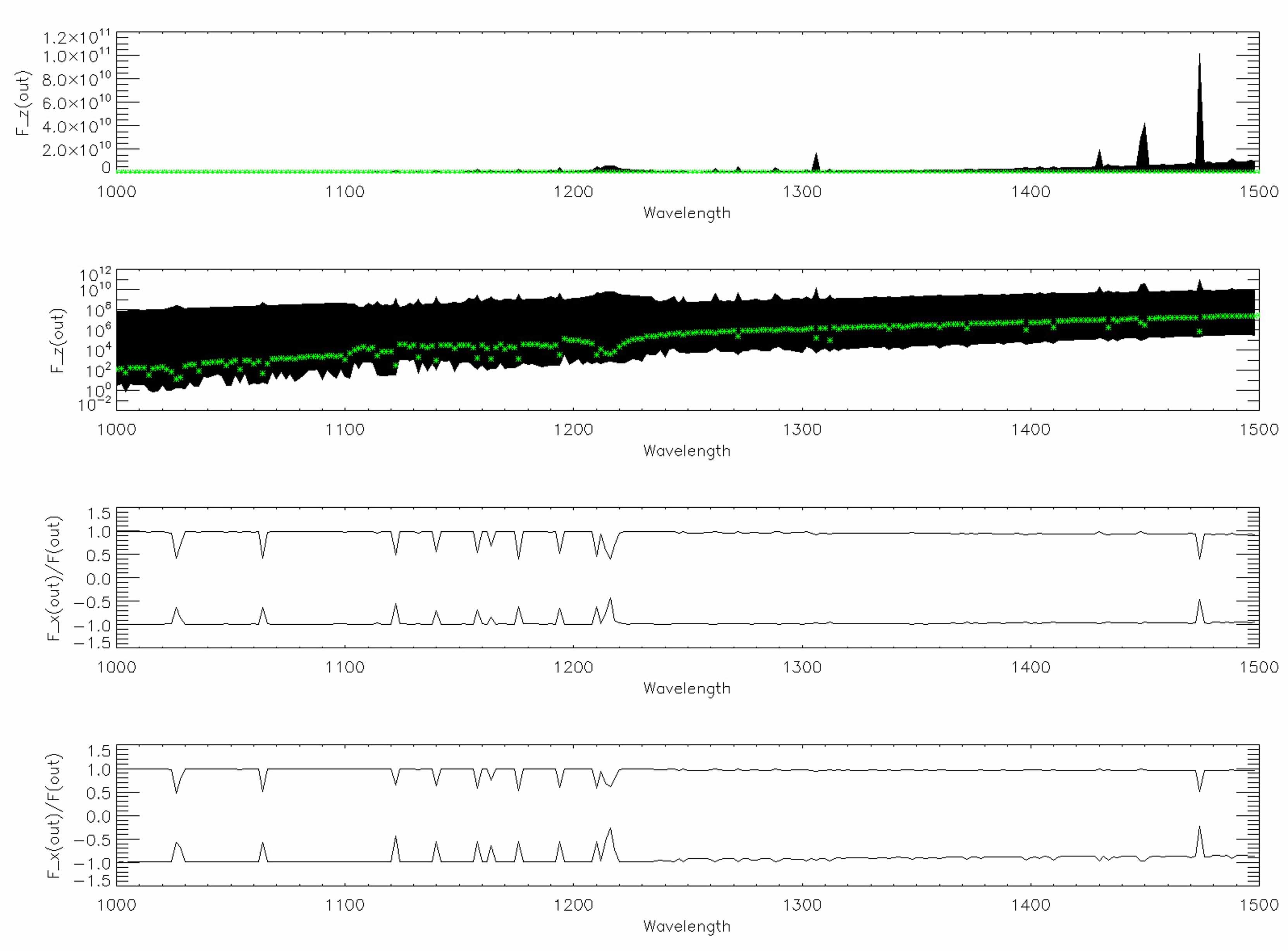 Figure 11
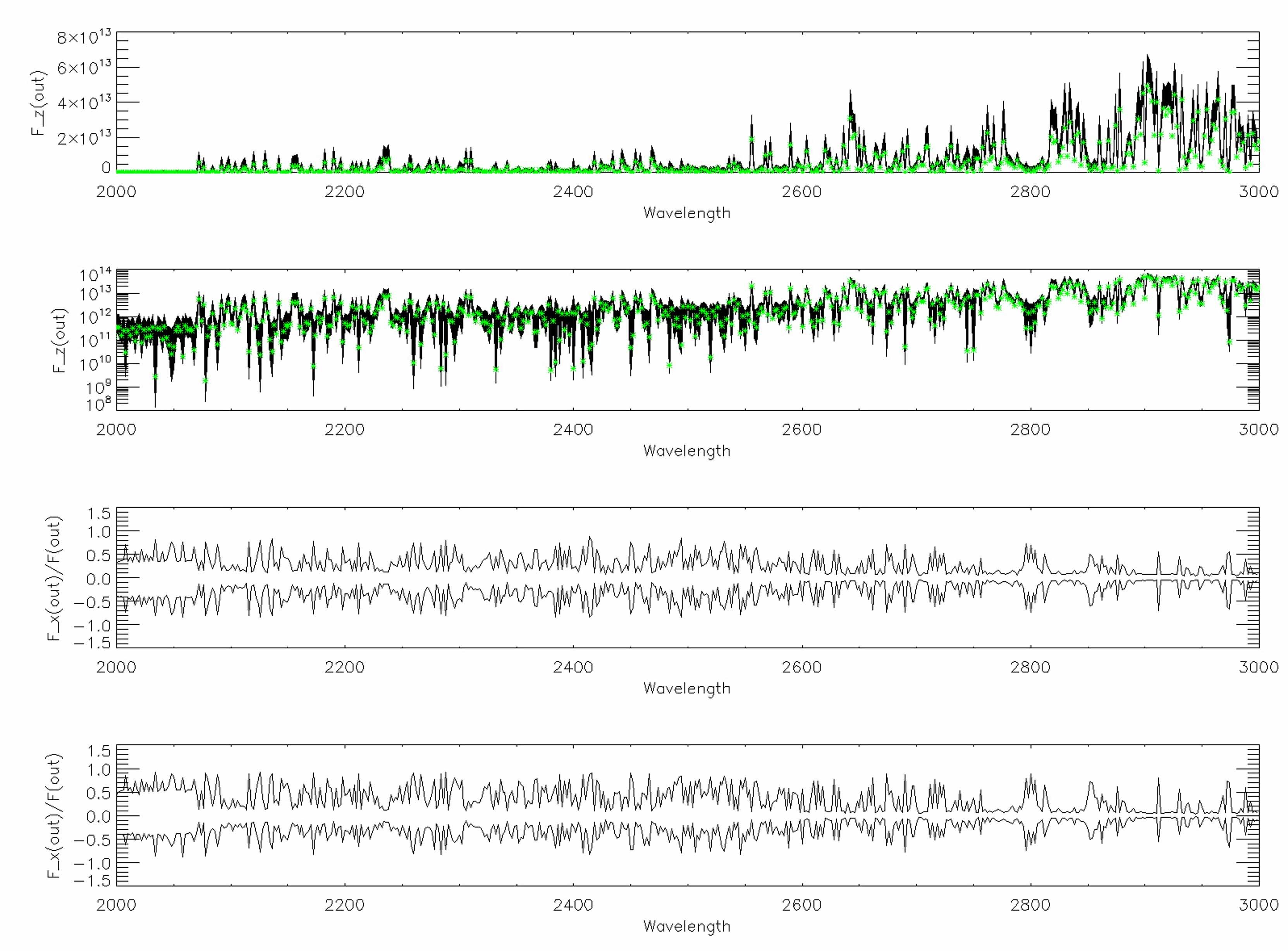 Figure 12
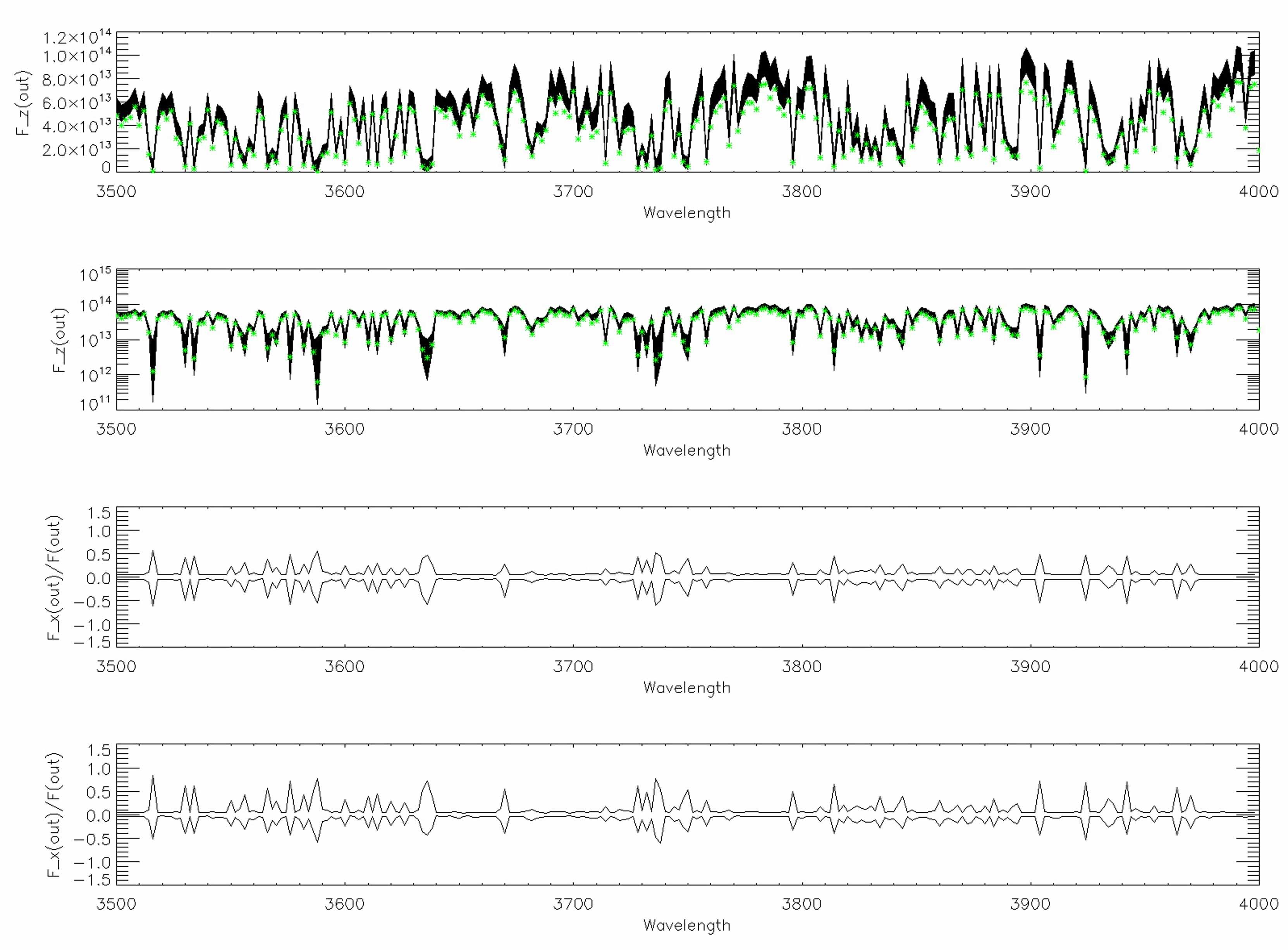 Figure 13
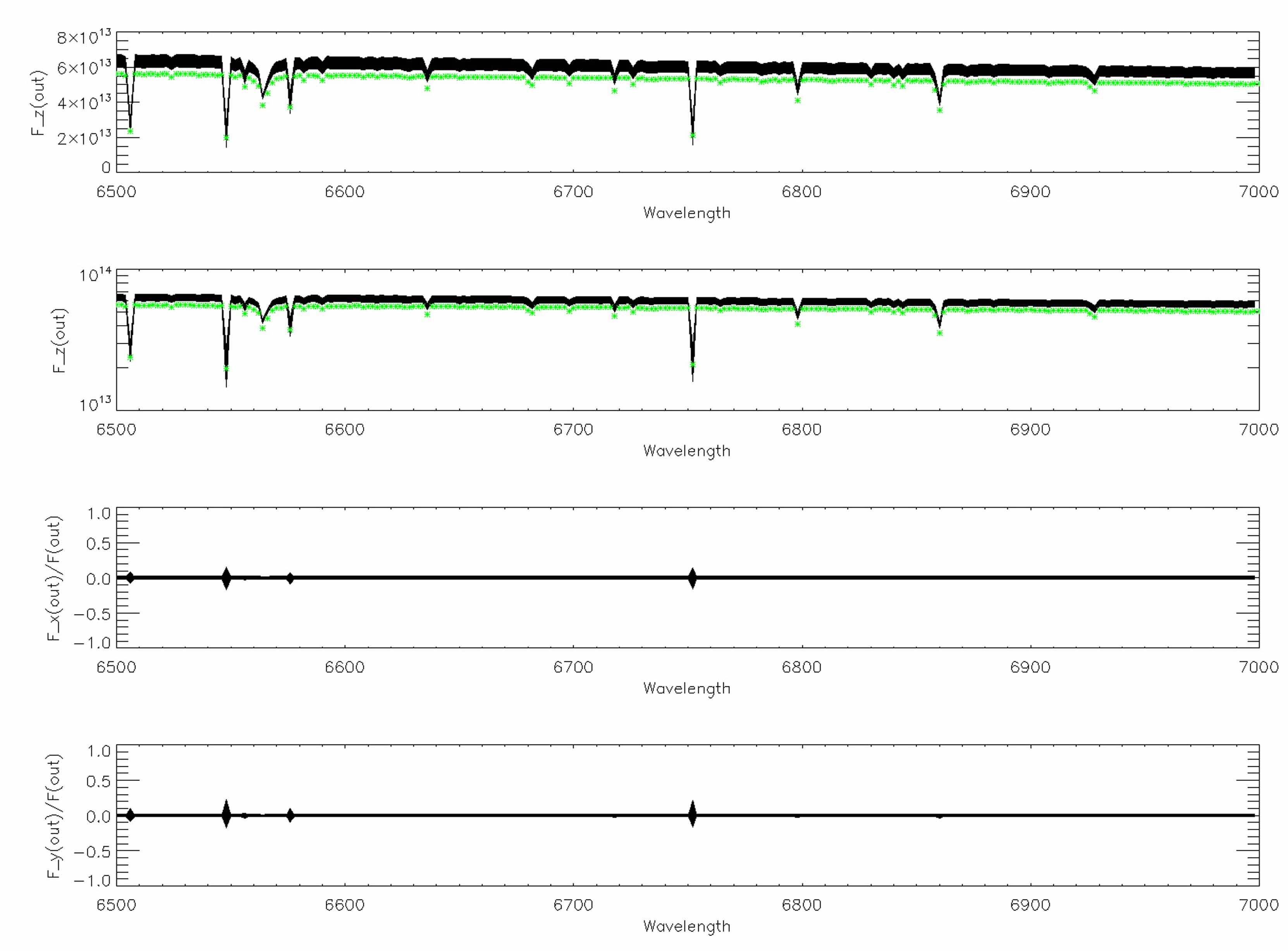 Figure 14
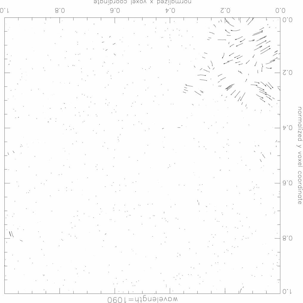 Figure 15
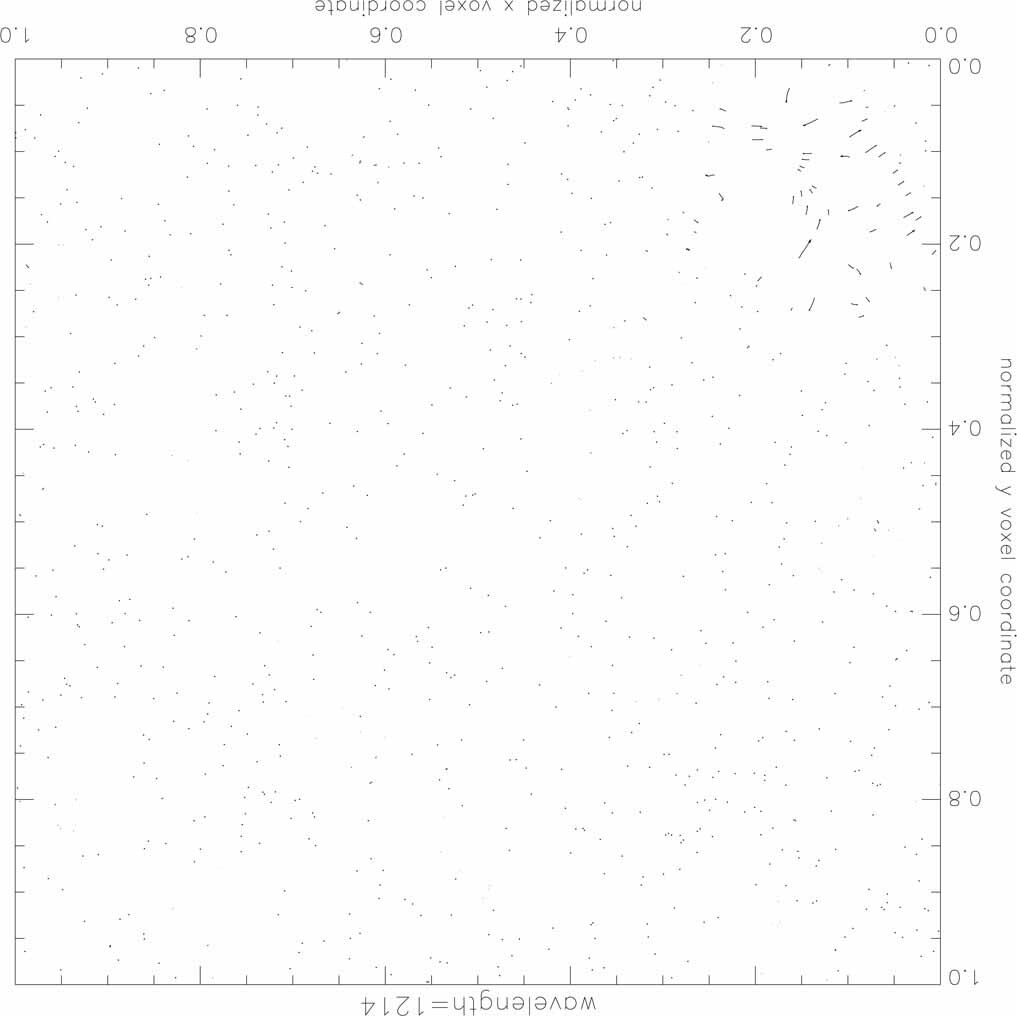 Figure 16
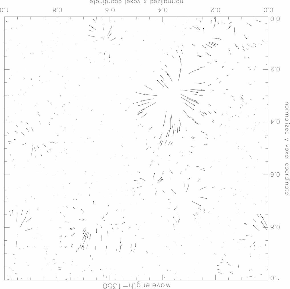 Figure 17
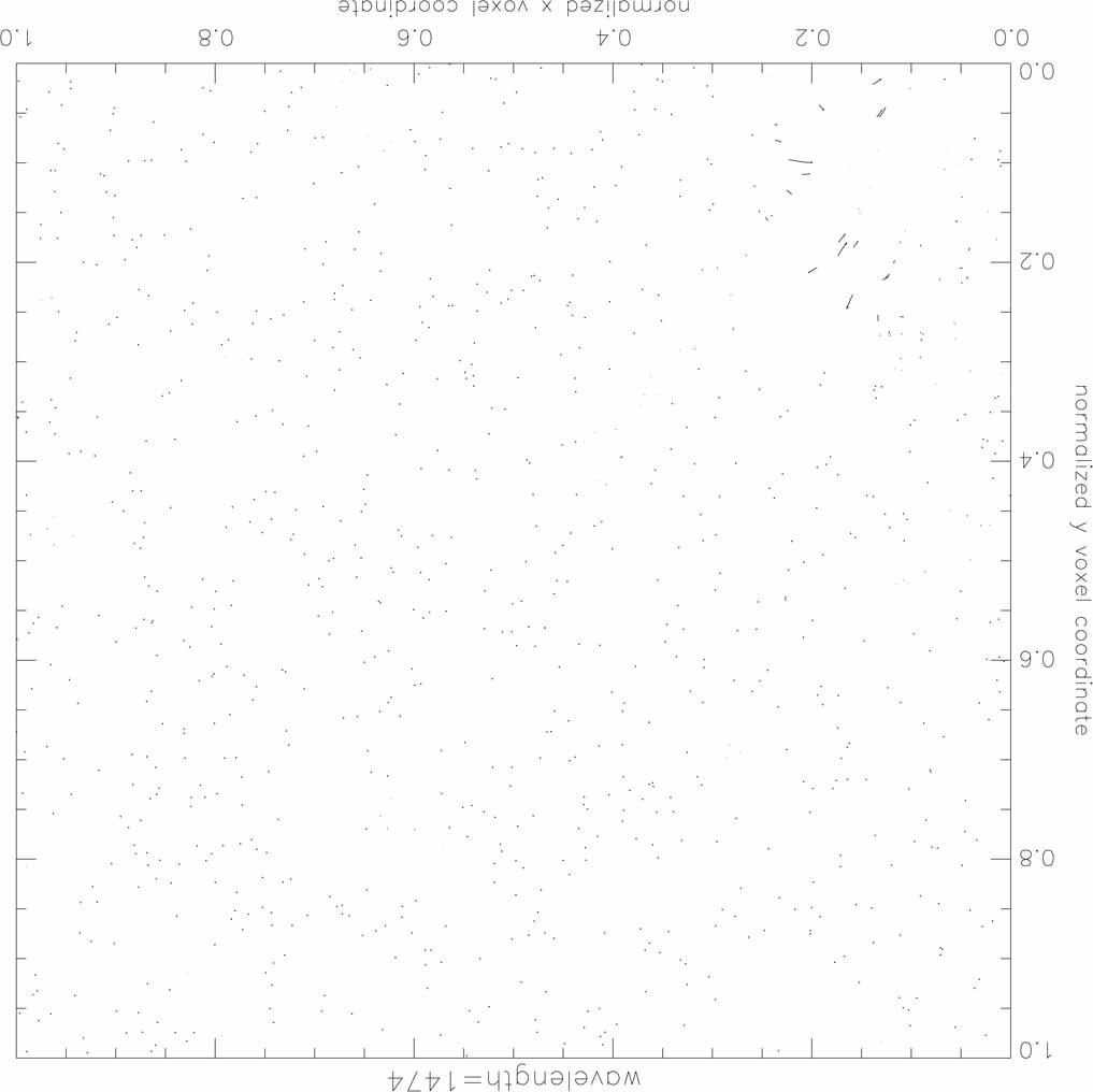 Figure 18
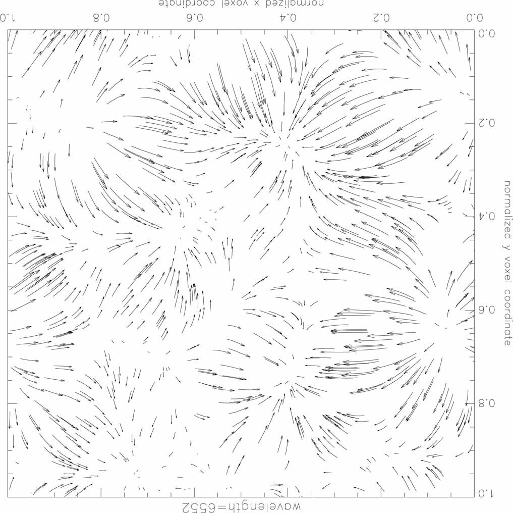 Figure 19
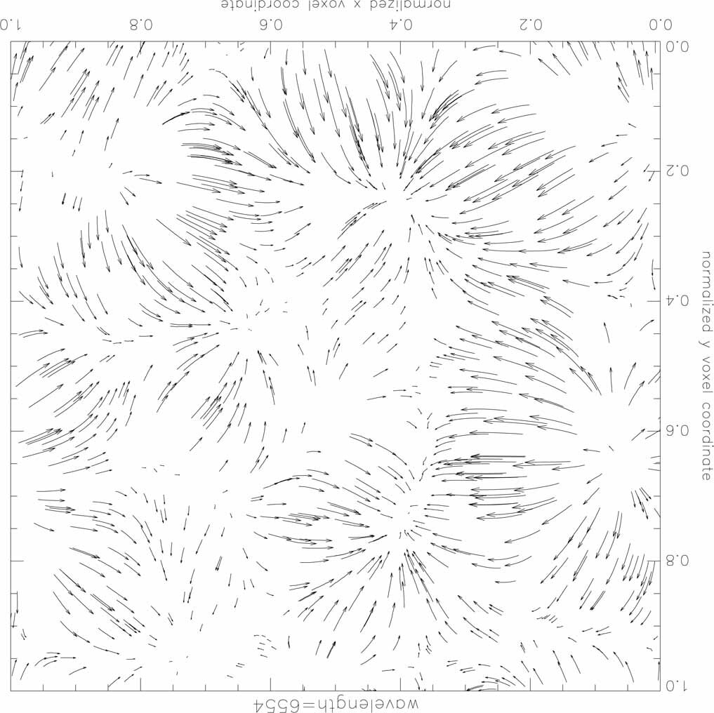 Figure 20
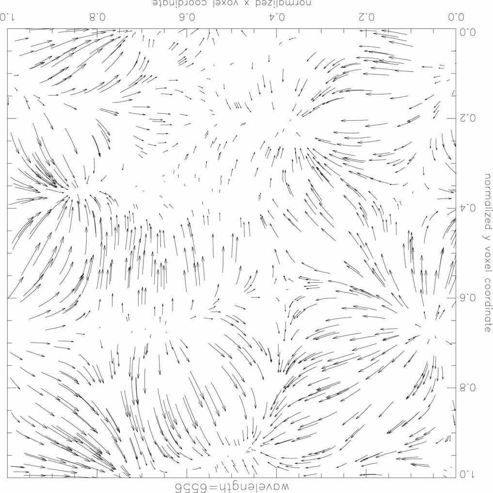 Figure 21
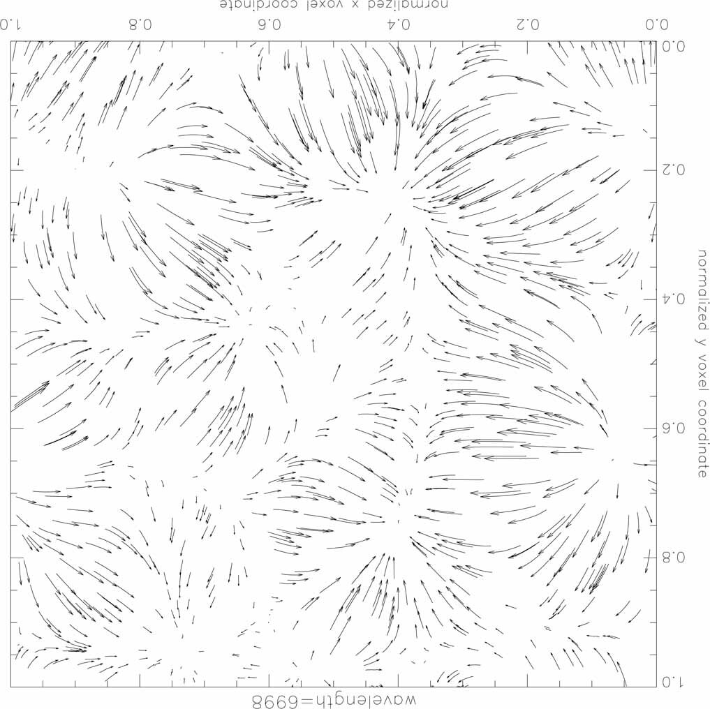 Figure 22
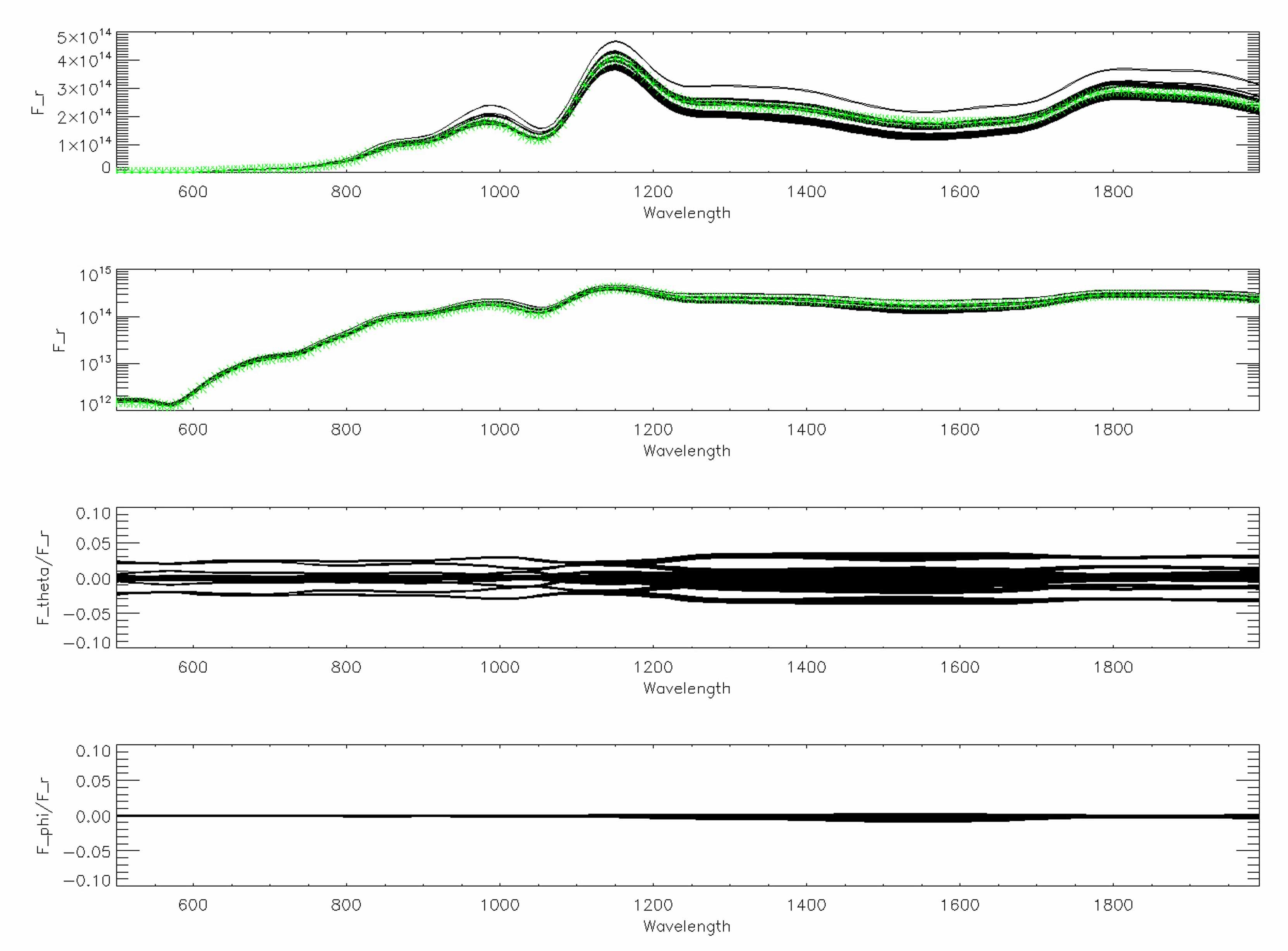 Figure 23
 Figure 24
| Timing: | Scaling: | |||||||||
|---|---|---|---|---|---|---|---|---|---|---|
| n(MPI) | cluster size | n(cluster) | line opacity | 3DRT | Comm | total | Line opacity | 3DRT | total | |
| 2048 | 512 | 4 | 2473 | 9942 | 436 | 12909 | 96.7% | 79.3% | 81.9% | |
| 2048 | 256 | 8 | 2414 | 8054 | 285 | 10789 | 99.1% | 97.9% | 98.0% | |
| 1024 | 512 | 2 | 4900 | 20103 | 754 | 25872 | 97.6% | 78.4% | 81.7% | |
| 1024 | 256 | 4 | 4741 | 15966 | 604 | 21385 | 100.9% | 98.7% | 98.9% | |
| 1024 | 128 | 8 | 4681 | 14275 | 471 | 19483 | 102.2% | 110.4% | 108.6% | |
| 512 | 512 | 1 | 9780 | 39793 | 1539 | 51341 | 97.8% | 79.2% | 82.4% | |
| 512 | 256 | 2 | 9566 | 31524 | 1061 | 42300 | 100.0% | 100.0% | 100.0% |
Peer Reviews
No public reviews on file for this paper yet. If you reviewed it on a platform where reviews are public (OpenReview, ICLR, NeurIPS, ICML), you can paste yours below so the community can read it here.
Videos
No videos yet. Explain this paper in a talk, walkthrough, or lecture? Add one.
Taxonomy
TopicsRadiative Heat Transfer Studies · Atmospheric aerosols and clouds · Urban Heat Island Mitigation
11institutetext: Hamburger Sternwarte, Gojenbergsweg 112, 21029 Hamburg, Germany; [email protected] 22institutetext: Homer L. Dodge Dept. of Physics and Astronomy, University of Oklahoma, 440 W. Brooks, Rm 100, Norman, OK 73019 USA; [email protected] 33institutetext: Computational Research Division, Lawrence Berkeley National Laboratory, MS 50F-1650, 1 Cyclotron Rd, Berkeley, CA 94720-8139 USA
A 3D radiative transfer framework: VI. PHOENIX/3D example applications
Peter H. Hauschildt and E. Baron 11112233
(Received date Accepted date)
Abstract
*Aims. *We demonstrate the application of our 3D radiative transfer framework in the model atmosphere code PHOENIX for a number of spectrum synthesis calculations for very different conditions.
*Methods. *The 3DRT framework discussed in the previous papers of this series was added to our general-purpose model atmosphere code PHOENIX/1D and an extended 3D version PHOENIX/3D was created. The PHOENIX/3D code is parallelized via the MPI library using a hierarchical domain decomposition and displays very good strong scaling.
*Results. *We present the results of several test cases for widely different atmosphere conditions and compare the 3D calculations with equivalent 1D models to assess the internal accuracy of the 3D modeling. In addition, we show the results for a number of parameterized 3D structures.
*Conclusions. *With presently available computational resources it is possible to solve the full 3D radiative transfer (including scattering) problem with the same micro-physics as included in 1D modeling.
Key Words.:
Radiative transfer – Scattering
1 Introduction
In a series of papers Hauschildt & Baron (2006, hereafter: Papers I–V); Baron & Hauschildt (2007, hereafter: Papers I–V); Hauschildt & Baron (2008, 2009, hereafter: Papers I–V); Baron, Hauschildt, & Chen (2009, hereafter: Papers I–V), we have described a framework for the solution of the radiative transfer equation in 3D systems (3DRT), including a detailed treatment of scattering in continua and lines with a non-local operator splitting method. These papers deal solely with the radiation transport problem and its numerical solution for test cases designed to stress-test the algorithms and codes. It is important, however, to apply the radiative transfer codes to ‘real’ problems, e.g., model atmosphere simulations and to compare the results to 1D equivalents. We have extended our general purpose model atmosphere code PHOENIX to use the 3DRT framework so that the new version of PHOENIX can calculate both 1D (PHOENIX/1D) and 3D (PHOENIX/3D) models and spectra. In this paper we will describe the implementation and the results of PHOENIX calculations comparing the results of 1D and 3D spectrum syntheses for different model parameters.
2 Method
In the following discussion we use notation of Papers I – V. The basic framework and the methods used for the formal solution and the solution of the scattering problem via non-local operator splitting are discussed in detail in these papers and will not be repeated here.
3 PHOENIX/3D implementation and micro-physics
We have implemented PHOENIX/3D to use as much as possible of the micro-physics of PHOENIX/1D. This applies to the ACES equation of state (Barman, in preparation), to the b-f and f-f opacities, to dust opacities, and to the line opacities (PHOENIX/3D is presently restricted to LTE population densities). This includes individual line profiles (Gauss profiles for weak lines and Voigt profiles for strong lines depending on user-selectable selection criteria) for atomic and molecular lines with the same physics that is implemented in PHOENIX/1D, so that the results of the opacity calculations are equal for the same physical conditions for the two modes of PHOENIX.
The important considerations of PHOENIX/3D implementation are memory and CPU time consumption. The memory requirements of PHOENIX/3D compared to PHOENIX/1D are mostly due the the much larger number of voxels in the 3D case (typically voxels) compared to the 1D case (usually 64–128 layers). As the memory required to store (and to compute) physical data such as the partial pressures of close to 900 species or the opacities scales linearly with the number of cells (or layers in 1D), it is obvious that only very small tests can be run without using domain decomposition methods on large scale parallel supercomputers. The domain decomposition implementation of PHOENIX/3D distributes the task of solving (and storing) the equation of state data and the wavelength dependent opacities to sets of processes each with its private memory. This linearly (with number of processes used) reduces the amount of memory and time required for these tasks. For 1024 processes, this reduces the memory requirements to just a few MB per process to store the full equation of state results. The 3DRT requires, in comparison, a total of about 450MB for the same problem (due to the storage requirements of the non-local -operator). Including the storage required for the computation of the line opacities, this is still just about 0.5GB/process, which is small compared to the typically available 4-16GB/core (CPU) on modern parallel supercomputers. In order to fully utilize the available memory per core and to increase flexibility we have implemented a hierarchical scheme similar to the parallel PHOENIX/1D implementation discussed in Hauschildt et al. (1997) and in Baron & Hauschildt (1998) and to the 3DRT parallelization in Paper II: We use a number of ‘clusters’ of processes where every cluster works on a different wavelength. Each cluster internally uses (on its subset of processes) the domain decomposition discussed above and the 3DRT parallelizations discussed in Paper I. This scheme can be adjusted to (a) fit the problem in the memory available for each core and (b) to optimize overall performances (e.g., depending on the number of solid angle points for the 3DRT solution or the coordinate system used). In the calculations presented here, we typically use clusters with 256–1024 processes, the number of clusters is limited only by the number of available CPUs.
4 Results
We have calculated a number of test models to compare the results of PHOENIX/1D calculations with PHOENIX/3D results. This comparison can be used to adjust the parameters of the 3D calculations (number of voxels or solid angle points) to give an accuracy that is acceptable for a given investment in computer time. The models that we show here were taken from the latest PHOENIX/1D grid (in preparation) of model atmospheres. In all stellar models (1D and 3D) we have used the set of solar abundances given in Asplund, Grevesse, & Sauval (2005).
4.1 Stellar Models
We have computed synthetic spectra for stellar model atmospheres with the parameters \hbox{,T_{\rm eff}}=3000{\rm K},\ {\log(g)}=5.0 (M dwarf), \hbox{,T_{\rm eff}}=5700{\rm K},\ {\log(g)}=4.5 (solar type star) and \hbox{,T_{\rm eff}}=9000{\rm K},\ {\log(g)}=4.5 (A star). The PHOENIX/1D models were computed with the latest setup in the input physics, including the ACES equation of state and the latest version of the atomic and molecular line databases. The model structures were then used as inputs to PHOENIX/3D to calculate synthetic spectra with the same sampling rates as the spectra from the PHOENIX/1D calculations. In the PHOENIX/3D calculations we have used a 3D spherical coordinate system with , and points for a total of about 1M voxels. The calculations used (if not specified otherwise) solid angle points. For each object we calculated synthetic spectra with PHOENIX/1D and PHOENIX/3D and compare the fluxes of the 1D spectra to the flux vectors of the 3D results. As in paper IV we can use the components of the 3D flux vector in 3D spherical coordinates to estimate the internal accuracy of the solution (as the and components are zero for spherically symmetric configurations). Figures 1 to 7 show selected results for the different models. In these cases, the error due to the number of solid angle points is about % and in all tests run the differences between the PHOENIX/1D fluxes and the component of the PHOENIX/3D calculation is of the same order. The differences between the 1D and 3D calculations are within the accuracy set by the number of solid angles in the 3D model. In order to verify that the errors get smaller with larger number of solid angles (as shown in Paper IV for simple test cases), we have run test models with angles. Three example plots are shown in Figs. 8 to 10 The results show clearly that the higher solid angle resolution reduces the errors in and considerably and also improves the comparison for to the 1D result, as the higher internal accuracy due to more solid angle points also increases the internal accuracy of . This also shows that in 3D radiative transfer calculations the spatial resolution is not the only factor governing the quality of the solution, the solid angle resolution may in fact be more important, depending on the coordinate system used and the details of the problem that isve calculated a number of test models to compare the results of PHOENIX/1D calculations with PHOENIX/3D results. This comparison can be used to adjust the parameters of the 3D calculations (number of voxels or solid angle points) to give an accuracy that is acceptable for a given investment in computer time. The models that we show here were taken from the latest PHOENIX/1D grid (in preparation) of model atmospheres. In all stellar models (1D and 3D) we have used the set of solar abundances given in Asplund, Grevesse, & Sauval (2005). We have calculated a number of test models to compare the results of PHOENIX/1D calculations with PHOENIX/3D results. This comparison can be used to adjust the parameters of the 3D calculations (number of voxels or solid angle points) to give an accuracy that is acceptable for a given investment in computer time. The models that we show here were taken from the latest PHOENIX/1D grid (in preparation) of model atmospheres. In all stellar models (1D and 3D) we have used the set of solar abundances given in Asplund, Grevesse, & Sauval (2005). being considered.
4.2 Scaling
In order to investigate the strong scaling properties of PHOENIX/3D we have constructed a small test case for a M dwarf model with 1000 wavelength points in a 3D spherical coordinate system with , and points for a total of about 1M voxels and solid angle points and ran the calculations with different configurations of the domain decomposition and different total numbers of processes. The total workload remains constant in these calculations, so this is a strong scaling test where the workload per CPU drops as the number of processes increase (in contrast to a weak scaling test where the workload per process remains constant). The results are given in Table 1. In this table, ‘n(MPI)’ is the total number of MPI processes used, ‘cluster size’ is the number of processes that collaboratively work on a single wavelength (spatial domain decomposition) and ‘n(cluster)’ is the number of such clusters, each working on a different wavelength (energy domain decomposition). The product ‘cluster size’ ‘n(cluster)’ is always equal to ‘n(MPI)’. The column ‘Comm’ gives the time spent in MPI communication to collect the opacities from the different processes before the 3DRT calculation starts. The communication requirements of the 3DRT calculations are included in the 3DRT column. The columns ‘line opacity’ give the time in seconds and scaling efficiency for all line opacity calculations, respectively, The columns ‘total’ give the total time and scaling efficiency, respectively, of the overall time spent in the computation of the 3D spectrum, this time does not include (small) contributions from the EOS solution and the line selection procedures. In the largest cluster size of 512 processes each process only works on 8 solid angles, whereas in the smallest cluster size (128) each process works on 32 solid angles. The work per solid angle is not perfectly constant and the amount of communication increases linearly as more processes collaborate, therefore, the scaling efficiency drops if more than about 512 processes are used for this problem size (i.e., number of solid angles). The scaling efficiency for the overall problem is quite good, the optimal value is about 98%. The drop-off for cluster sizes of 512 (and more) is due to (a) the relatively small number of solid angles leading to very little work for each 3DRT process and relatively more internal communication time in the 3DRT and (b) the small effect of the communication related to the spatial domain decomposition. We could not test setups with more than (the maximum available) 2048 processes; however, the test case should scale to 256k processes (number of wavelength points times cluster size), although for such a setup the overheads for, e.g., the solution of the equation of state and the line selection would be very noticeable.
4.3 3D hydro model of solar convection
For a test with a computed 3D structure, we use the same example snapshot structure from H-G. Ludwig Caffau et al. (2007); Wedemeyer et al. (2004) of a radiation-hydrodynamical simulation of convection in the solar atmosphere as in Paper III. The radiation transport calculations were performed with a total of Cartesian grid points in , , and , respectively, for a total of voxels, the periodic boundary conditions are set in the (horizontal) plane. The 3D radiative transport equation is solved for and solid angle points, so that a total of about intensities are calculated for each 3DRT iteration and wavelength point. For the tests described here, we are only using the temperature–pressure structure of the hydro model and ignore the velocity field.
We show example results in Figs. 11 to 14 in terms of the , , and components of the flux vectors of each outer boundary voxel. The components are, in addition, compared to the 1D model for the G2V star with the parameters \hbox{,T_{\rm eff}}=5700{\rm K},\ {\log(g)}=4.5 ( symbols in the figures). The general shape of the 3D spectra compare well to the 1D solar type model, of course there are large variations across the horizontal plane. In the UV the differences are largest, a number of voxel flux vectors show strong line emission, whereas the radiative+convective equilibrium 1D model only shows absorption features. This is to be expected as the 3D simulation of convection gives significant temperature variations across the volume considered, in particular in the horizontal plane. These variations have considerable effect on the radiative transfer solution: The horizontal components of the flux vectors of each voxel compared to the length of the flux vector , and , show quite substantial variations for different wavelengths. The variations are much larger for smaller wavelengths (e.g., in the UV), due to the larger temperature dependence of the source functions for smaller wavelengths which translates to larger horizontal flux components for small wavelengths compared to longer wavelengths.
The components of the flux vectors in the plane can be larger than the component, strongly dependent on the wavelength and on the location of the voxel. This is illustrated in Figs. 15 – 22, which show the flowlines of the components of the flux vector at the surface. The flow distances are much larger at optical wavelengths than in the UV due to the larger UV opacities. The ‘pattern’ of the horizontal energy flow depends strongly on the wavelength, it is also significantly different in the cores of strong lines compared to the surrounding continuum. The horizontal heat exchange could have in turn noticeable effects on the gas flow pattern.
4.4 Supernovae
The modeling of supernova spectra is a very important application of PHOENIX/3D modeling as it is expected, and explosion models show, that supernova explosions are intrinsically 3D driven. For the calculations shown here we use the Lagrangian frame 3DRT in spherical 3D coordinates as discussed in paper V. The test model is a simplified model for a type II supernova atmosphere with a maximum expansion speed of about . The model is a simple uniform composition model with the density parameterized as , and a “photospheric velocity” of km s*-1*, and a model temperature of K. These conditions correspond roughly to those of SN 1999em seven days after explosion. In Fig. 23 we show the CMF spectrum of the PHOENIX/3D run compared to the corresponding PHOENIX/1D synthetic spectrum. Due to computer time limitations we could only run a relatively small 3D model with , and points and solid angle points. The small angular resolution causes the scatter in the plots and the errors in the and components. In general the agreement is acceptable for this test run, for a full scale 3D SN spectrum the resolution in should be increased to at least and the angular resolution should be at least (which reduces the bandwidth dramatically, see Paper V).
5 Summary and Conclusions
We have described first results we have obtained by incorporating the 3D radiative transfer framework we have discussed in Papers I-V into our general purpose model atmosphere package PHOENIX, thus allowing both 1D models (PHOENIX/1D) and 3D models (PHOENIX/3D) with the same micro-physics. We have verified and tested PHOENIX/3D by computing a number of test spectra for 1D conditions and comparing the results to the corresponding PHOENIX/1D calculations. The conditions range from M dwarfs, solar type stars to A stars and Type II supernovae with relativistic expansions speeds. In addition, we have calculated spectra for a 3D hydrodynamical simulation of solar atmosphere convection. These tests demonstrate the it is now possible to calculate realistic spectra for 3D configurations including complex micro-physics. PHOENIX/3D can be used to calculate synthetic spectra for a number of complex 3D atmosphere model, including irradiated stars or planets, novae, and supernovae. We are currently working on extensions of the 3D radiative transfer framework to arbitrary velocity fields in the Euler (for low velocities, e.g., in convection simulations or planetary winds) and the Lagrangian (for Supernovae, accretion disks and matter flow in the vicinity of black holes) frames, which will extend the applications of PHOENIX/3D significantly.
Acknowledgements.
This work was supported in part by DFG GrK 1351 and SFB 676, as well as NSF grant AST-0707704, and US DOE Grant DE-FG02-07ER41517. The calculations presented here were performed at the Höchstleistungs Rechenzentrum Nord (HLRN); at the Hamburger Sternwarte IBM Regatta Systems, Apple G5, and Delta Opteron clusters financially supported by the DFG and the State of Hamburg; and at the National Energy Research Supercomputer Center (NERSC), which is supported by the Office of Science of the U.S. Department of Energy under Contract No. DE-AC03-76SF00098. We thank all these institutions for a generous allocation of computer time.
The reference list from the paper itself. Each links out to its DOI / PubMed record.
- 1Asplund et al. (2005) Asplund, M., Grevesse, N., & Sauval, A. J. 2005, in ASP Conf. Ser. 336: Cosmic Abundances as Records of Stellar Evolution and Nucleosynthesis, ed. T. G. Barnes, III & F. N. Bash, 25
- 2Baron & Hauschildt (1998) Baron, E. & Hauschildt, P. H. 1998, Ap J, 495, 370
- 3Baron & Hauschildt (2007) Baron, E. & Hauschildt, P. H. 2007, A&A, 468, 255
- 4Baron et al. (2009) Baron, E., Hauschildt, P. H., & Chen, B. 2009, A&A, 498, 987
- 5Caffau et al. (2007) Caffau, E., Steffen, M., Sbordone, L., Ludwig, H.-G., & Bonifacio, P. 2007, A&A, 473, L 9
- 6Hauschildt & Baron (2006) Hauschildt, P. H. & Baron, E. 2006, A&A, 451, 273
- 7Hauschildt & Baron (2008) Hauschildt, P. H. & Baron, E. 2008, A&A, 490, 873
- 8Hauschildt & Baron (2009) Hauschildt, P. H. & Baron, E. 2009, A&A, 498, 981