Solving the Einstein field equations
A.V.Bratchikov

TL;DR
This paper presents a perturbative method to solve Einstein's vacuum field equations, providing a graphical diagrammatic representation of the solutions to facilitate understanding and computation.
Contribution
It introduces a novel perturbation-based approach with a diagrammatic visualization for solving Einstein's equations.
Findings
Successful construction of solutions using perturbation theory
Diagrammatic representation simplifies understanding of solutions
Provides a new computational framework for Einstein's equations
Abstract
A solution of the Einstein vacuum field equations is constructed within the contex of perturbation theory. The solution possesses a graphical representation in terms of diagrams.
Click any figure to enlarge with its caption.
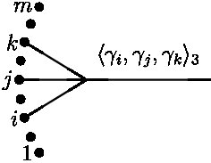 Figure 1
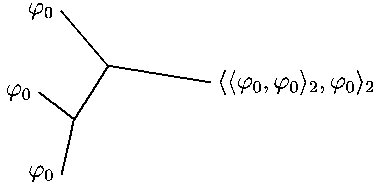 Figure 2
Peer Reviews
No public reviews on file for this paper yet. If you reviewed it on a platform where reviews are public (OpenReview, ICLR, NeurIPS, ICML), you can paste yours below so the community can read it here.
Videos
No videos yet. Explain this paper in a talk, walkthrough, or lecture? Add one.
Taxonomy
TopicsComputational Physics and Python Applications · Algebraic and Geometric Analysis
Solving the Einstein field equations
A.V.Bratchikov
Kuban State Technological University,
2 Moskovskaya Street, Krasnodar, 350072, Russia
Abstract
A solution of the Einstein vacuum field equations is constructed within the contex of perturbation theory. The solution possesses a graphical representation in terms of diagrams.
In a recent article [1] for a wide class of nonlinear equations a perturbative solution was constructed.This class includes equations of motion of field theories. Solutions of the pure Yang-Mills field equations and equations of motions in spinor electrodynamics [2] were obtained. The solutions can be described by diagrams. The aim of the present paper is to construct a solution of the Einstein field equations in the vacuum.
Let be space-time coordinates, and a space-time metric. The vacuum Einstein equations read
[TABLE]
where
[TABLE]
is the Ricci tensor
[TABLE]
and is the Cristofel symbol
[TABLE]
For we can expand equations (1) in powers of
[TABLE]
Here
[TABLE]
We impose a gauge condition
[TABLE]
where
[TABLE]
From equation (4) it follows
[TABLE]
Let be defined by Then equation (2) takes the form [3]
[TABLE]
where
The general solution of the free equation
[TABLE]
is given by [4]
[TABLE]
where
[TABLE]
are coordinates on the unit sphere , is the area element on
[TABLE]
[TABLE]
and are some functions. Equation (3) implies
[TABLE]
A specific solution of the inhomogeneous equation
[TABLE]
reads
[TABLE]
Then equation (6) can be written in the form
[TABLE]
where and Here we introduced an auxiliary parameter . Eventually it is set to be
Let be the space of symmetric 2-forms. We shall need the polylinear symmetric functions
[TABLE]
defined for by
[TABLE]
One can check that
[TABLE]
Then equation (7) becomes
[TABLE]
For let
[TABLE]
be defined by
[TABLE]
where means that is omitted. If is given by
[TABLE]
for some we say that is a descendant of
Each descendant can be represented by a diagram. In this diagram an element of is represented by the line segment . A product
[TABLE]
is represented by the vertex joining the line segments for The general rule for graphical representation of should be clear from Figure 1.Here we show the diagram for
[TABLE]
The points labeled by represent the ends of the lines for Using the representation for one can consecutively draw the diagrams for (10).
Let us introduce a family of functions
[TABLE]
such that for is defined as the sum of all the descendants of its arguments. For example, for and we have
[TABLE]
[TABLE]
A solution of equation (9) is given by [1]
[TABLE]
where
[TABLE]
is defined as [math] if and otherwise
[TABLE]
For example, the contribution in is given by
[TABLE]
The diagram for is depicted in Figure 2.
The tensor can be found by using (5).
The reference list from the paper itself. Each links out to its DOI / PubMed record.
- 1[1] A.V.Bratchikov, Perturbation theory for nonlinear equations, ar Xiv 0910.3924 [hep-th].
- 2[2] A.V.Bratchikov, Solving field equations in spinor electrodynamics, ar Xiv 0910.0621 [hep-th].
- 3[3] L.D.Landau and D.V.Lifshits, The classical theory of fields, Nauka, Moscow, 1973.
- 4[4] R.Courant and D.Hilbert, Methods of mathematical physics, Wiley, 1989.