Computation of Maxwell's equations on Manifold using DEC
Zheng Xie, Yujie Ma

TL;DR
This paper presents a numerical method using discrete exterior calculus to solve Maxwell's equations on manifolds, analyzing stability and errors, with implementation for simulating electromagnetic waves in vacuum.
Contribution
Introduces a discrete exterior calculus approach for Maxwell's equations on manifolds, including stability analysis and implementation details.
Findings
Stable numerical scheme for Maxwell's equations on manifolds
Error analysis of the discretization method
Simulation of TE/M waves in vacuum
Abstract
In this paper, the method of discrete exterior calculus for numerically solving Maxwell's equations in space manifold and the time is discussed, which is a kind of lattice gauge theory. The analysis of its stable condition and error is also accomplished. This algorithm has been implemented on C++ plateform for simulating TE/M waves in vacuum.
Click any figure to enlarge with its caption.
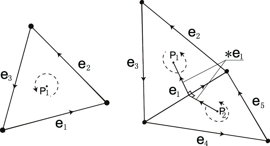 Figure 1
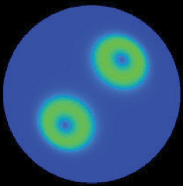 Figure 2
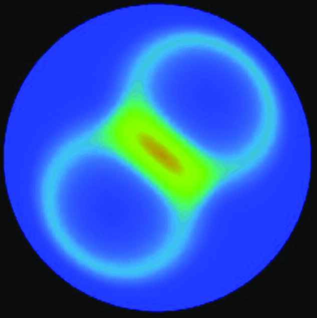 Figure 3
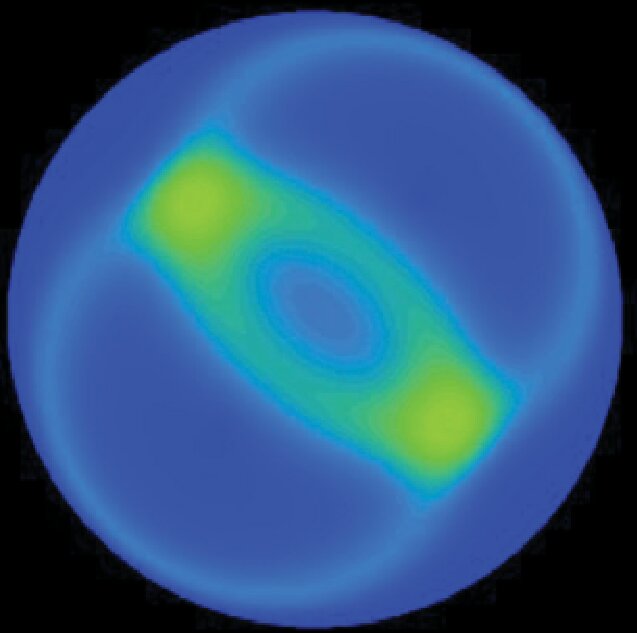 Figure 4
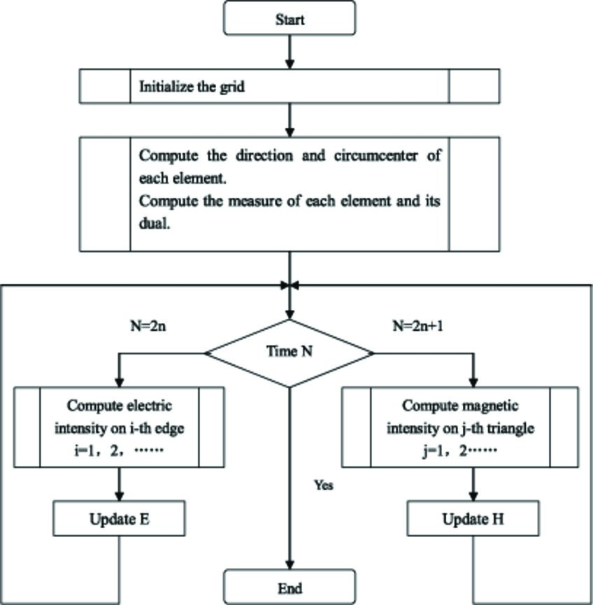 Figure 5
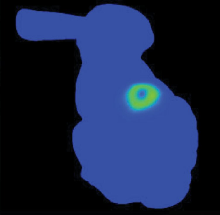 Figure 6
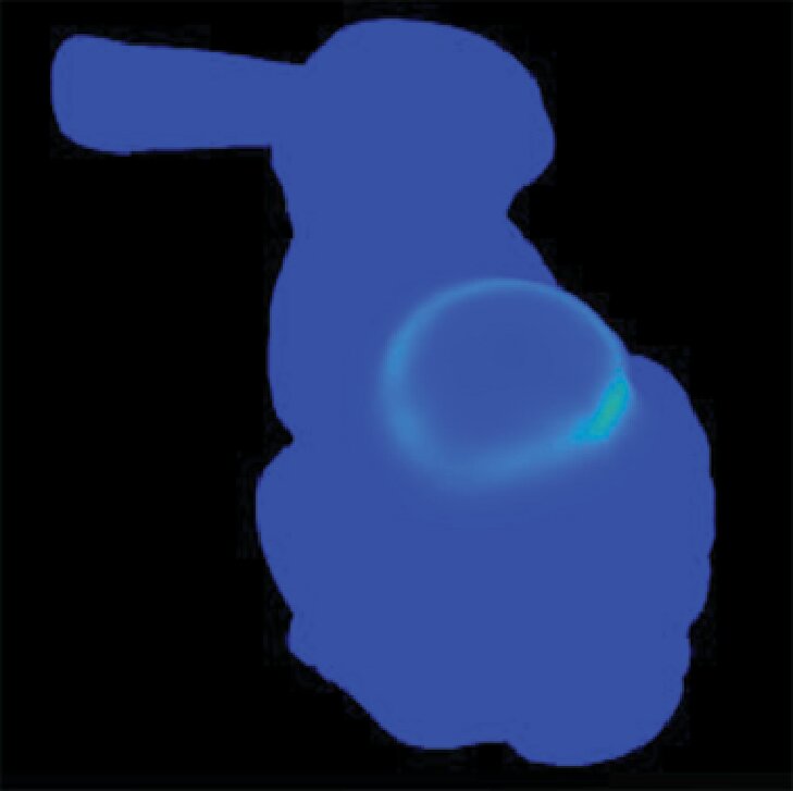 Figure 7
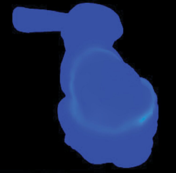 Figure 8
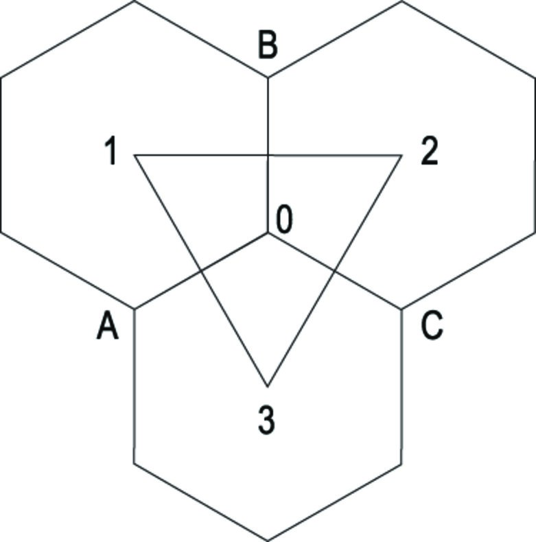 Figure 9
Peer Reviews
No public reviews on file for this paper yet. If you reviewed it on a platform where reviews are public (OpenReview, ICLR, NeurIPS, ICML), you can paste yours below so the community can read it here.
Videos
No videos yet. Explain this paper in a talk, walkthrough, or lecture? Add one.
Taxonomy
TopicsElectromagnetic Simulation and Numerical Methods · Advanced Numerical Methods in Computational Mathematics · Numerical methods for differential equations
Computation of Maxwell’s equations on Manifold using DEC
Zheng Xie1 Yujie Ma2
Center of Mathematical Sciences, Zhejiang University (310027),China
Key Laboratory of Mathematics Mechanization,
Chinese Academy of Sciences, (100090), China E-mail: [email protected] E-mail: [email protected] This work is partially supported by CPSFFP (No. 20090460102), NKBRPC (No. 2004CB318000), and NNSFC (No. 10871170)
Abstract
In this paper, the method of discrete exterior calculus for numerically solving Maxwell’s equations in space manifold and the time is discussed, which is a kind of lattice gauge theory. The analysis of its stable condition and error is also accomplished. This algorithm has been implemented on C++ plateform for simulating TE/M waves in vacuum.
**Keywords: **Discrete exterior calculus, Discrete variation, Maxwell’s equations, Lattice gauge theory.
PACS(2010): 41.20.Jb, 02.30.Jr, 02.40.Sf, 02.60.Cb.
1 Introduction
Computational electromagnetism is concerned with the numerical study of Maxwell’s equations. The Yee scheme is known as finite difference time domain and is one of the most successful numerical methods, particularly in the area of microwave problems[1]. It preserves important structural features of Maxwell’s equations[2, 3, 4, 5, 6]. Bossavit et al present the Yee-like scheme and extend Yee scheme to unstructured grids. This scheme combines the best attributes of the finite element method (unstructured grids) and Yee scheme (preserving geometric structure)[7, 8]. Stern et al [9] generalize the Yee scheme to unstructured grids not just in space, but in 4-dimensional spacetime by discrete exterior calculus(DEC)[10, 11, 14, 15, 16, 20, 17, 18, 19, 12, 13]. This relaxes the need to take uniform time steps.
In this paper, we generalize the Yee scheme to the discrete space manifold and the time. The spacetime manifold used here is split as a product of D time and D or D space manifold. The space manifold can be approximated by triangular and tetrahedrons depending on dimension, and the time by segments. So the spacetime manifold is approximated by prism lattice, on which the discrete Lorentz metric can be defined.
With the technique of discrete exterior calculus, the value discrete connection, curvature and Bianchi identity are defined on prim lattice. With discrete variation of an inner product of discrete forms and their dual forms, the discrete source equation and continuity equation are derived.
- 2.
Those equations compose the discrete Maxwell’s equations in vacuum case, which just need the local information of triangulated manifold such as length and area.
The discrete Maxwell’s equations here can be re-grouped into two sets of explicit iterative schemes for TE and TM waves, respectively. Those schemes can directly use acute triangular, rectangular, regular polygon and their combination, which has been implemented on C++ plateform to simulate the electromagnetic waves propagation and interference on manifold.
2 DEC for Maxwell’s equations
Maxwell’s equations can be simply expressed once the language of exterior differential forms is used. The electric and magnetic fields are jointly described by a curvature form in a 4-D spacetime manifold. The Maxwell’s equations reduce to the Bianchi identity and the source equation
[TABLE]
where denotes the exterior differential operator, denotes the Hodge star operator, and 1-form is called the electric current form satisfying the continuity equation
[TABLE]
As the exterior derivative is defined on any manifold, the differential form version of the Bianchi identity makes sense for any 3D or 4D spacetime manifold, whereas the source equation is defined if the manifold is oriented and has a Lorentz metric. Now, we introduce the discrete counterpart of those differential geometric objects to derive the numerical computational schemes for Maxwell’s equations.
Discrete Lorentz metric
The spacetime manifold used here is split as a product of D time and D or D space manifold. The D or D space manifold can be approximated by triangular or tetrahedrons, and the time by segments. The length of edge and area of triangular and volume of tetrahedrons gives the discrete Riemann metric on space grids. The metric on time grid is the minus of length square. The spacetime manifold is approximated by prism lattice, on which the discrete Lorentz metric can be defined as the product of discrete metric on space and time.
Discrete exterior calculus
A discrete differential -form, , is the evaluation of the differential -form on all -simplices. Dual forms, i.e., forms that we evaluate on the dual cell. Suppose each simplex contains its circumcenter. The circumcentric dual cell of simplex is
[TABLE]
where is all the simplices which contains ,…, , and is the circumcenter of .
The two operators in Eqs.(1) can be discretized as follows:
Discrete exterior differential operator , this operator is the transpose of the incidence matrix of -cells on -cells.
- 2.
Discrete Hodge Star , the operator scales the cells by the volumes of the corresponding dual and primal cells.
Discrete connection and curvature
Discrete connection form or gauge field assigns to each element in the set of edges an element of the gauge group :
[TABLE]
Discrete curvature form is the discrete exterior derivative of the discrete connection form
[TABLE]
The value of on each element in the set of triangular is the coefficient of Holonomy group of this face. The form automatically satisfies the discrete Bianchi identity
[TABLE]
Note that since the gauge group used here is abelian, we need not pick a starting vertex for the loop. We may traverse the edges in any order, so long as taking orientations into account.
Discrete Maxwell’s equations
For source case, we need discrete current form . Let and the Lagrangian functional be
[TABLE]
where
[TABLE]
Supposing that there is a variation of , vanishing on the boundary, we have
[TABLE]
The Hamilton’s principle of stationary action states that this variation must equal zero for any such vary of , implying the Euler-Lagrange equations
[TABLE]
which is the discrete source equation
[TABLE]
where . Since , the discrete continuity equation can express as:
[TABLE]
The equations of discrete Bianchi identity (2), source equation (3), and continuity equation (4) are called discrete Maxwell’s equations.
Discrete Gauge transformations
Discrete gauge transformations are maps
[TABLE]
for any form or scalar function on vertex. Since the discrete exterior derivative maps
[TABLE]
the discrete Maxwell’s equations(2-4) are invariant under discrete gauge transformations. Since the discrete continuity equation (4) ensures
[TABLE]
so we have
[TABLE]
That is to say the Lagrangian function is also invariant under discrete gauge transformations.
3 Explicit schemes
Schemes for TE wave
The discrete current form, discrete curvature form and its dual can be written as
[TABLE]
where and denote the coordinate of the time, (electric field) is discrete form on space, (magnetic field) is discrete form on space, (magnetizing field) is the dual of on space, (electric displacement field) is the dual of on space, (charge density) is the discrete form on time, (electric current density) is the discrete form on space. The discrete Maxwell’s equations can be rewritten as
[TABLE]
where , are the restriction of , on space, and
[TABLE]
If allowing for the possibility of magnetic charges and current discrete form
[TABLE]
the symmetric scheme can be written as
[TABLE]
where
- (magnetic charges) is discrete 3-form on space,
- (current) is discrete form on space.
The compact form of Eqs.(6) can be written as
[TABLE]
with discrete continuity equations or integrability conditions
[TABLE]
Proposition 3.1
If the initial condition satisfies the first and third equations in Eqs.(6), the solution of the second and fourth equations in Eqs.(6) automatically satisfy Eqs.(6).
Proof. Because the dimension of spacetime is , therefore
[TABLE]
and the continuity equations can be reduced to
[TABLE]
So we have
[TABLE]
Now we show the scheme (5) on the product of 2D discrete space manifold and time. The second and fourth equations in Eqs.(5) based on Fig.1 are
[TABLE]
where denotes the measure of forms and dual. The summation on the right is orient, that is to say, inverse the orientation of , then multiply with . Eqs.(7) can be implemented on 2D discrete manifold directly(see Fig.1). Eq.(7) on rectangular gird is just the Yee scheme.
[TABLE]
In the absence of magnetic or dielectric materials, the relations are simple:
[TABLE]
where and are two universal constants, called the permittivity of free space and permeability of free space, respectively. With relations (8), Eqs.(7) can be rewritten into an explicit iterative scheme for TE wave.
[TABLE]
The symmetric TE wave scheme induced from Eqs.(6) can be written as follows.
[TABLE]
Schemes for TM wave
If writing
[TABLE]
where is the discrete form on space, is the discrete form on space, is the dual of on space, is the dual of on space, is the discrete form on space, is the discrete form on space, is the discrete form on time, is the discrete form on space, the discrete Maxwell’s equations can be rewritten as
[TABLE]
Proposition 3.2
If the initial condition satisfies the first and third equations in Eqs.(11), the solution of the second and fourth equations in Eqs.(11) automatically satisfy Eqs.(11).
Proof.Because the dimension of spacetime is or , therefore
[TABLE]
and the continuity equations can be reduced to
[TABLE]
So we have
[TABLE]
Now we show the scheme (11) on the product of 2D discrete space manifold and time. The second and fourth equations in Eqs.(11) based on Fig.1 are
[TABLE]
With relations (8), Eqs.(12) can be rewritten into an explicit iterative scheme for TM wave.
[TABLE]
General schemes
For real world materials, the constitutive relations are not simple proportionalities, except approximately. The relations can usually still be written:
[TABLE]
but and are not, in general, simple constants, but rather functions. With Ohm’s law
[TABLE]
where is the electrical conductivity and is magnetic conductivity. The DEC schemes can be written as
[TABLE]
[TABLE]
4 Stability, convergence and accuracy
Stability
The Courant-Friedrichs-Lewy condition is a necessary condition for convergence while solving certain partial differential equations numerically. Now, we find this condition for scheme (10). Condition for scheme (13) can be induced in the same way. First, we decompose DEC algorithm into temporal and spacial eigenvalue problems.
The temporal eigenvalue problem:
[TABLE]
It can approximated by difference equation
[TABLE]
Supposing
[TABLE]
and
[TABLE]
and substituting those into Eq.(14), we obtain
[TABLE]
[TABLE]
therefore
[TABLE]
This is the stabile condition for the temporal eigenvalue problem.
The spacial eigenvalue problem:
[TABLE]
It can be approximated by difference equation (15) based on Fig.2.
[TABLE]
[TABLE]
Let
[TABLE]
and substitute into Eq.(15) to obtain
[TABLE]
[TABLE]
So we have
[TABLE]
In order to keep the stability of scheme (13), we need
[TABLE]
or
[TABLE]
Convergence
By the definition of truncation error, the exact solution of Maxwell’s equations satisfy the same relation as DEC scheme except for an additional term . This expresses the consistency, and so convergence for DEC scheme by Lax equivalence theorem (consistency stability convergence).
Accuracy
The derivative of Maxwell’s equations is approximated by first order difference in schemes (10) and (13). Equivalently, and are approximated by linear interpolation functions. Consulting the definition about accuracy of finite volume method, we can also say that schemes (10) and (13) have first order spacial and temporal accuracy, and have second order spacial and temporal accuracy on rectangular grid with equivalent space and time steps.
5 Implementation
The DEC algorithm of Maxwell’s equations was implemented in C++ platform. The Fig.3 shows the flowchart of DEC schemes for Maxwell’s equations.
[TABLE]
In the common practice, not every simulation step needs to be visualized, especially when the time step size is too small. Fig.4 exhibit Gaussian pluses’ waveforms simulated by DEC.
[TABLE]
Fig.5 exhibits two sources Gaussian pluses interference simulated by DEC. Our algorithm can simulate more complex situation on surface and 3D-space manifold.
[TABLE]
The reference list from the paper itself. Each links out to its DOI / PubMed record.
- 1[1] K.S. Yee, Numerical solution of inital boundary value problems involving Maxwell’s equations in isotropic media. IEEE Trans. Ant. Prop. 14(3), 302-307 (1966).
- 2[2] A. Bondeson, T. Rylander, P. Ingelstrom, Computational electromagnetics, Texts in Applied Mathematics, vol. 51. Springer, New York (2005).
- 3[3] M. Clemens, T. Weiland, Magnetic field simulation using conformal FIT formulations. IEEE Trans. Magn. 38(2), 389-392 (2002).
- 4[4] P.W. Gross, P.R. Kotiuga, Electromagnetic theory and computation: a topological approach, Mathematical Sciences Research Institute Publications, vol. 48. Cambridge University Press, Cambridge, (2004).
- 5[5] E. Hairer, C. Lubich, G. Wanner, Geometric numerical integration, Springer Series in Computational Mathematics, vol. 31. Springer-Verlag, Berlin (2002).
- 6[6] A. Nicolet, F. Zolla, Y.O. Agha and S. Guenneau, Geometrical transformations and equivalent materials in computational electromagnetism, International Journal for Computation and Mathematics in Electrical and Electronic Engineering COMPEL, vol. 27, 806-819, (2008).
- 7[7] A. Bossavit, L. Kettunen, : Yee-like schemes on a tetrahedral mesh, with diagonal lumping. Int. J. Numer. Modell. 12(1-2), 129 142 (1999).
- 8[8] A. Bossavit, L. Kettunen, Yee-like schemes on staggered cellular grids: A synthesis between FIT and FEM approaches. IEEE Trans. Magn. 36(4), 861 867 (2000).