2-torsion in the n-solvable filtration of the knot concordance group
Tim D. Cochran (Rice University), Shelly Harvey (Rice University) and, Constance Leidy (Wesleyan University)

TL;DR
This paper demonstrates that for the n-solvable filtration of the knot concordance group, the associated graded groups contain infinitely many elements of order 2, with specific properties and distinctions based on classical invariants.
Contribution
It proves the existence of infinitely many 2-torsion elements in the graded groups of the n-solvable filtration, expanding prior knowledge from lower levels to higher levels.
Findings
Each G_n contains infinite 2-torsion elements for n>1.
These elements are represented by negative amphichiral knots with trivial classical invariants.
The knots are distinguished by their Alexander polynomials and higher-order Alexander modules.
Abstract
In 1997 Cochran-Orr-Teichner introduced a natural filtration, called the n-solvable filtration, of the smooth knot concordance group, C. Its terms {F_n} are indexed by half integers. We show that each associated graded abelian group G_n=F_n/F_{n.5}, n>1, contains infinite linearly independent sets of elements of order 2 (this was known previously for n=0,1). Each of the representative knots is negative amphichiral, with vanishing s-invariant, tau-invariant, delta-invariants and Casson-Gordon invariants. Moreover each is smoothly slice in a rational homology 4-ball. In fact we show that there are many distinct such classes in G_n, distinguished by their classical Alexander polynomials and by the orders of elements in their higher-order Alexander modules.
Click any figure to enlarge with its caption.
 Figure 1
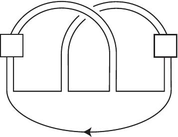 Figure 2
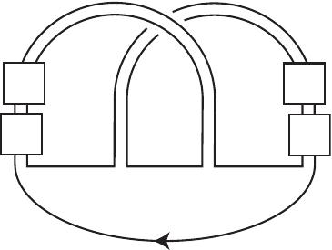 Figure 3
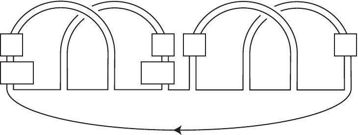 Figure 4
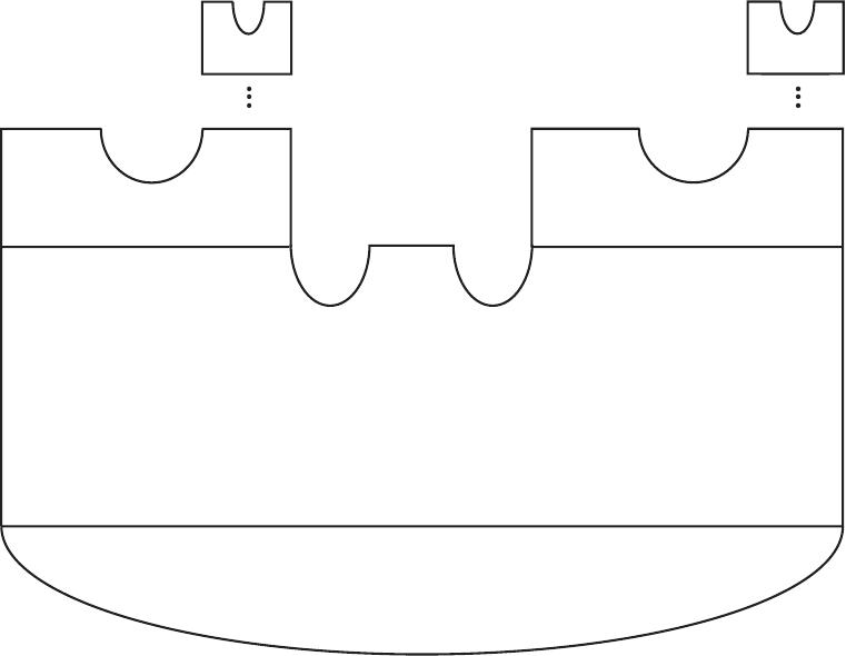 Figure 5
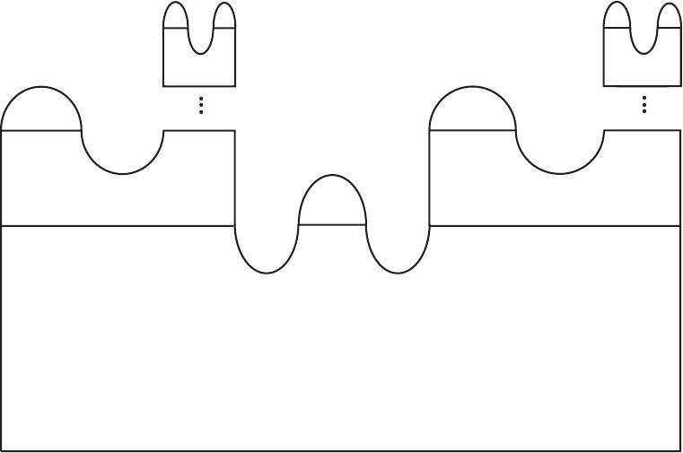 Figure 6
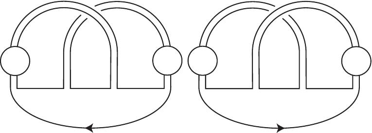 Figure 7
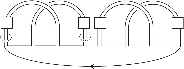 Figure 8
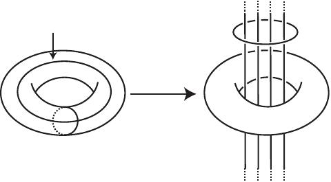 Figure 9
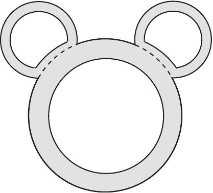 Figure 10
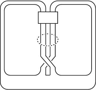 Figure 11
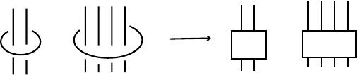 Figure 12
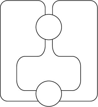 Figure 13
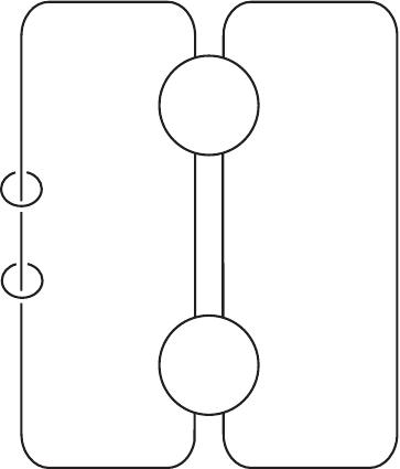 Figure 14
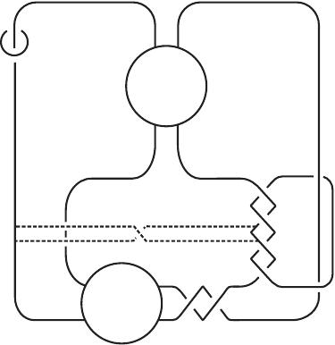 Figure 15
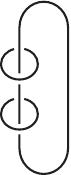 Figure 16
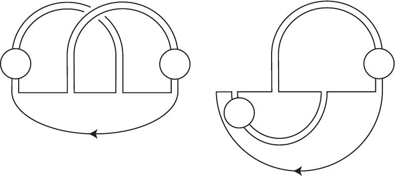 Figure 17
Peer Reviews
No public reviews on file for this paper yet. If you reviewed it on a platform where reviews are public (OpenReview, ICLR, NeurIPS, ICML), you can paste yours below so the community can read it here.
Videos
No videos yet. Explain this paper in a talk, walkthrough, or lecture? Add one.
2-Torsion in the -Solvable Filtration of the Knot concordance group
Tim D. Cochran*†*
Department of Mathematics MS-136, P.O. Box 1892, Rice University, Houston, TX 77251-1892
,
Shelly Harvey*††*
Department of Mathematics MS-136, P.O. Box 1892, Rice University, Houston, TX 77251-1892
and
Constance Leidy*†††*
Department of Mathematics, Wesleyan University, Wesleyan Station, Middletown, CT 06459
Abstract.
Cochran-Orr-Teichner introduced in [11] a natural filtration of the smooth knot concordance group
[TABLE]
called the ()-solvable filtration. We show that each associated graded abelian group , contains infinite linearly independent sets of elements of order (this was known previously for ). Each of the representative knots is negative amphichiral, with vanishing -invariant, -invariant, -invariants and Casson-Gordon invariants. Moreover each is slice in a rational homology -ball. In fact we show that there are many distinct such classes in , distinguished by their Alexander polynomials and, more generally, by the torsion in their higher-order Alexander modules.
2000 Mathematics Subject Classification:
Primary 57M25; Secondary 20J
*†*Partially supported by NSF DMS-0706929
*††*Partially supported by NSF CAREER DMS-0748458
*†††*Partially supported by NSF DMS-0805867
1. Introduction
A (classical) knot is the image of a smooth embedding of an oriented circle in . Two knots, and , are concordant if there exists a proper smooth embedding of an annulus into that restricts to the knots on . Let denote the set of (smooth) concordance classes of knots. The equivalence relation of concordance first arose in the early ’s in work of Fox, Kervaire and Milnor in their study of isolated singularities of -spheres in -manifolds and, indeed, certain concordance problems are known to be equivalent to whether higher-dimensional surgery techniques “work” for topological -manifolds [15][28][3]. It is well-known that can be endowed with the structure of an abelian group (under the operation of connected-sum), called the smooth knot concordance group. The identity element is the class of the trivial knot. Any knot in this class is concordant to a trivial knot and is called a slice knot. Equivalently, a slice knot is one that is the boundary of a smooth embedding of a -disk in . In general, the abelian group structure of is still poorly understood. But much work has been done on the subject of knot concordance (for excellent surveys see [19] and [37]). In particular, [11] introduced a natural filtration of by subgroups
[TABLE]
called the ()-solvable filtration of and denoted (defined in Section 3). The non-triviality of can be measured in terms of the associated graded abelian groups (here we ignore the other “half” of the filtration, , where almost nothing is known). This paper is concerned with elements of order two in and, more generally, with elements of order two in .
We will review some of the history of -torsion phenomena in in the context of the -solvable filtration. One of the earliest results concerning was an epimorphism constructed by Fox and Milnor [15]
[TABLE]
Soon thereafter, Levine constructed an epimorphism
[TABLE]
to a group, , that became known as the algebraic knot concordance group. Any knot in the kernel of (1.1) is called an algebraically slice knot. In terms of the -solvable filtration, Levine’s result is [11, Remark 1.3.2, Thm. 1.1]:
[TABLE]
It is known that there exist elements of order two in that realize some of the above -torsion invariants. Let denote the mirror image of the oriented knot , obtained as the image of under an orientation reversing homeomorphism of ; and let denote the reverse of , which is obtained by merely changing the orientation of the circle. Then it is known that is a slice knot, so the inverse of in , denoted , is represented by , denoted . A knot is called negative amphichiral if is isotopic to . It follows that, for any negative amphichiral knot , is a slice knot, since it is isotopic to . Hence negative amphichiral knots represent elements of order either or in . It is a conjecture of Gordon that every class of order two in can be represented by a negative amphichiral knot [19].
In fact the work of Milnor and Levine in the ’s resulted in a more precise statement:
[TABLE]
where the sum is over all primes where and [34, Sections 10,11,24][48][24, p.131]. That is, the algebraic concordance group (and ) admits a certain -primary decomposition, wherein a knot has a nontrivial -primary part only if is a factor of its Alexander polynomial. (Indeed, Levine and Stoltzfus classified by first splitting the Witt class of the Alexander module (with its Blanchfield form) into its -primary parts).
In the ’s the introduction of Casson-Gordon invariants in [1][2] led to the discovery that the subgroup of algebraically slice knots was of infinite rank and contained infinite linearly independent sets of elements of order two [27][36]. In terms of the -solvable filtration this implies the existence of
[TABLE]
Different -summands were exhibited in [31][16]. More recent work of Se-Goo Kim [29] on the “polynomial splitting” properties of Casson-Gordon invariants led to a generalization analogous to the result of Milnor-Levine:
[TABLE]
Thus there is evidence that also exhibits a -primary decomposition. Further strong evidence is given in [30]. Although a similar statement for the -torsion in has not appeared, it is expected from combining the work of [29] and Livingston [36]. Several authors have shown that certain knots that projected to classes of order and in are in fact of infinite order in [38][39][26][20][35]. A number of papers have addressed the non-triviality of , [18][17][31][16][11][12][13], culminating in [10] where it was shown that, for any integer , there exists
[TABLE]
Moreover the recent work [8] of the authors resulted in a generalization of the latter fact, along the lines of the Levine-Milnor primary decomposition and [30]: for each “distinct” -tuple of prime polynomials with , there is a distinct subgroup , yielding a subgroup
[TABLE]
Given a knot , such an -tuple encodes the orders of certain submodules of the sequence of higher-order Alexander modules of . Thus one can distinguish concordance classes of knots not only by their classical Alexander polynomials, but also, loosely speaking, by their higher-order Alexander polynomials. This result indicates that decomposes not just according to the prime factors of the classical Alexander polynomial, but also according to types of torsion in the higher-order Alexander polynomials.
Here we show corresponding results for -torsion. That is, for any , not only will we exhibit
[TABLE]
but we also will exhibit many distinct such subgroups
[TABLE]
parametrized by their Alexander polynomials and the types of torsion in the higher-order Alexander polynomials. The representative knots are distinguished by families of von Neumann signature defects associated to their classical Alexander polynomials and “higher-order Alexander polynomials”. The precise statement is given in Theorem 5.8. Each of these concordance classes has a negative amphichiral representative that is smoothly slice in a rational homology -ball. Thus the classical signatures and the Casson-Gordon signature-defect obstructions [1] (indeed all metabelian obstructions) vanish for these knots [11, Theorem 9.11]. In addition, the -invariant of Rasmussen [45], the -invariant of Ozsváth-Szabó [43], and the invariants of Manolescu-Owens and Jabuka [41][25][42] vanish on these concordance classes, since each of these invariants induces a homomorphism and so must have value zero on classes representing torsion in . Our examples are inspired by those of Livingston, who provided examples that can be used to establish (1.3) in the case [36]. His examples are distinguished by their Casson-Gordon signature defects. Our examples are distinguished by higher-order -signature defects. It is striking that elements of finite order can sometimes be detected by signatures. The key observation is that, unlike invariants such as the classical knot signatures, the invariant, the -invariant, or the -invariants, the invariants arising from higher-order signature defects (including Casson-Gordon invariants) are not additive under connected sum. Therefore there is no reason to expect that they would vanish on elements of finite order.
Our work is further evidence that exhibits some sort of primary decomposition, but wherein not only the classical Alexander polynomial, but also some higher-order Alexander polynomials are involved.
We remark that [11] also defined a filtration, , of the topological concordance group, . Since it is known, by work of Freedman and Quinn, that a knot lies in if and only if it lies in , all of the results of this paper apply equally well, without change, to the filtration . Therefore, for simplicity, in this paper we will always work in the smooth category.
2. The examples
Our examples are inspired by those of Livingston [36], who exhibited an infinite “linearly independent” set of negative amphichiral algebraically slice knots. His examples can be used to establish the existence of the aforementioned
[TABLE]
2.1. The Building Blocks
Consider the knot shown on the left-hand side of Figure 2.1.
Here is an arbitrary pure two component string link [32][21]. The disk containing the letter symbolizes replacing the trivial -string link by the -string link . Viewing the knot diagram as being in the -plane ( being vertical), the mirror image can be defined as the image under the reflection , which alters a knot diagram by replacing all positive crossings by negative crossings and vice-versa. Recall that the image of under this reflection is denoted . We also consider a “flip” homeomorphism of which flips over a diagram, given by rotation of degrees about the -axis or . Note that these homeomorphisms commute. Special cases of the following elementary observation appeared in [36, Lemma 2.1] [37, p.326] and [4, p. 60].
Lemma 2.1**.**
Suppose is an arbitrary pure two component string link. Then the knot on the left-hand side of Figure 2.1 is negative amphichiral.
Proof.
The knot on the right-hand side of Figure 2.1 is a diagram for , since it is obtained by a reflection, in the plane of the paper, of the diagram for , followed by a reversal of the string orientation. Here we use that commutes with the reflection. We claim that the result is isotopic to . Flipping the diagram (rotating by degrees about the vertical axis in the plane of the paper), we arrive at the diagram shown on the left-hand side of Figure 2.2. This is identical to the original diagram of except that the left-hand band passes under the right-hand band instead of over. But the left-hand band can be “swung” around by an isotopy as suggested in the right-hand side of Figure 2.2, bringing it on top of the other band, at which point one arrives at the original diagram of . ∎
The following result was shown for the figure-eight knot (the case that the string link is a single twist) by the first author (inspired by [14]). It was extended, by Cha, to the case that is an arbitrary number of twists in [4, p.63]. Our contribution here is just to note that Cha’s proof suffices to prove this more general result.
Lemma 2.2**.**
Each knot in the family shown in Figure 2.1 is slice in a rational homology -ball.
Proof.
We follow the argument of [4], only indicating where our more general argument deviates. It suffices to show that the zero-framed surgery, , as shown on the left-hand side of Figure 2.3, is rational homology cobordant to . After adding, to , a four-dimensional -handle and -handle (going algebraically twice over the -handle) and performing certain handle slides (see [4, p.62-64]), one arrives at a -manifold given by surgery on the -component link drawn as the solid lines on the right-hand side of Figure 2.3. Therefore is rationally homology cobordant to .
Next one shows, as follows, that this underlying -component link, , is concordant to the simple -component link, shown on the right-hand side of Figure 2.4.
Ignoring the framings on , add a band as shown by the dashed lines on the right-hand side of Figure 2.3, resulting in the -component link, , shown on the left-hand side of Figure 2.4. Here is the image of the (unoriented) string link under the map . One must be careful here since , which is reflection in the plane of the paper, is not the correct notion of mirror image for a string link. Since our -axis is the true axis of the string link (the factor in ), is the concordance inverse of in the string link concordance group [32][22], so is concordant to the trivial -string link. Hence the link is concordant to the -component link, , that would result from taking to be trivial. Capping off the right-most unknotted component of , we arrive at the -component link, , shown on the right-hand side of Figure 2.4. This describes the desired concordance from to . Consequently, is homology cobordant to the -manifold described by the framed link on the right-hand side of Figure 2.4, which is known to homeomorphic to . ∎
In this paper we will only need the special case of these lemmas wherein the string link consists of two twisted parallels of a single knotted arc as indicated by the examples in Figures 2.5 and 2.6. Here an inside the rectangle indicates full positive twists between the two strands, and the inside the rectangle indicates that the trivial two component string link has been replaced by two parallel zero-twisted copies of a single knotted arc . This is explained more fully in Subsection 2.2.
Proposition 2.3**.**
If and are distinct positive integers then the Alexander polynomials of and of are distinct and irreducible, hence coprime.
Proof.
A Seifert matrix for with respect to the obvious basis is
[TABLE]
Thus the Alexander polynomial of is . The discriminant is easily seen, for , to never be the square of an integer, so the roots of are real and irrational. Hence is irreducible over . It follows that if and had a common factor then they would be identical up to a unit. But the equations and imply so . ∎
2.2. Doubling Operators
To construct knots that lie deep in the -solvable filtration, we use iterated generalized satellite operations.
Suppose is a knot in and be an ordered, oriented, trivial link in , that misses , bounding a collection of oriented disks that meet transversely as shown on the left-hand side of Figure 2.7. Suppose is an -tuple of auxiliary knots. Let denote the result of the operation pictured in Figure 2.7, that is, for each , take the embedded disk in bounded by ; cut off along the disk; grab the cut strands, tie them into the knot (such that the strands have linking number zero pairwise) and reglue as shown schematically on the right-hand side of Figure 2.7.
We will call this the result of infection performed on the knot using the infection knots along the curves [12]. In the case that this is the same as the classical satellite construction. This construction has an alternative description. For each , remove a tubular neighborhood of in and glue in the exterior of a tubular neighborhood of along their common boundary, which is a torus, in such a way that (the longitude of) is identified with the meridian, , of and the meridian of is identified with the reverse of the longitude, , of as suggested by Figure 2.8. The resulting space can be seen to be homeomorphic to and the image of is the new knot.
It is well known that if the input knots and are concordant, then the output knots and are concordant. Thus the functions descend to .
Definition 2.4** ([9, 8]).**
A doubling operator, is a function, as in Figure 2.7, that is given by infection on a ribbon knot wherein, for each , . Often we suppress from the notation.
These are called doubling operators because they generalize untwisted Whitehead doubling.
In particular we will consider the family of doubling operators shown in Figure 2.9.
Note that, since is negative amphichiral by Lemma 2.1,
[TABLE]
which is well known to be a ribbon knot [46, Exercise 8E.30]. Thus is a negative amphichiral ribbon knot. For the case , this was already noted in [36].
We will also consider the family of doubling operators, , shown in Figure 2.10 (where here the inside a box symbolizes full negative twists between the bands but where the individual bands remain untwisted), equipped with a specified circle that can be shown to generate its Alexander module.
2.3. Elements of order 2 in
Now we describe large families of examples of negative amphichiral knots that lie in . Let be any knot with Arf(). Let be the image of under the composition of any doubling operators (each requiring a single input), that is,
[TABLE]
Then, for any integer we define as in Figure 2.11, that is, .
Proposition 2.5**.**
For any , any , any composition of doubling operators and any Arf invariant zero input knot , the knot of Figure 2.11 satisfies
- •
* is negative amphichiral;*
- •
;
- •
* is (smoothly) slice in a smooth rational homology -ball; and*
- •
* is a slice knot.*
Proof.
It was shown in [10, Theorem 7.1] that, for any any doubling operator ,
[TABLE]
Since any knot of Arf invariant zero is known to lie in [11, Remark 8.14,Thm. 8.11], and since is the image of under a composition of doubling operators, it follows that .
Note that is the connected sum of two knots each of which is of the form shown in Figure 2.6 (hence of the form of Figure 2.1). Thus, by Lemma 2.2, each such is slice in a rational homology -ball. Moreover, by Lemma 2.1, is negative amphichiral so is isotopic to . But the latter is a ribbon knot and hence a slice knot. ∎
For specificity we define the following infinite families:
Definition 2.6**.**
Given an -tuple of integers and an Arf invariant zero knot , we define to be the image of under the following composition of doubling operators. Specifically let
[TABLE]
as shown in Figure 2.11, where is
[TABLE]
where the are the operators of Figure 2.10. In other words, we recursively set:
[TABLE]
Even though depends on , we will often suppress the latter from the notation.
3. Commutator Series and Filtrations of the knot concordance groups
To accomplish our goals, we must establish that many of the knots in the families given by Figure 2.11, and specifically those in Definition 2.6, are not in and, indeed, are distinct from each other in . To this end we review recent work of the authors that introduced refinements of the -solvable filtration parameterized by certain classes of group series that generalized the derived series. In particular the authors defined specific filtrations of that depend on a sequence of polynomials. These filtrations can then be used to distinguish between knots with different Alexander modules or different higher-order Alexander modules. All of the material in this section is a review of the relevant terminology of [8, Sections 2,3].
Recall that the derived series, , of a group is defined recursively by and . The rational derived series [23], , is defined by and
[TABLE]
More generally,
Definition 3.1** ([8, Definition 2.1]).**
A commutator series defined on a class of groups is a function, , that assigns to each group in the class a nested sequence of normal subgroups
[TABLE]
such that is a torsion-free abelian group.
Proposition 3.2** ([8, Proposition 2.2]).**
For any commutator series ,
* (and in particular , whence the name commutator series);*
- 2.
, that is, every commutator series contains the rational derived series;
- 3.
* is a poly-(torsion-free abelian) group (abbreviated PTFA);*
- 4.
* and are right (and left) Ore domains.*
Any commutator series that satisfies a weak functoriality condition induces a filtration, , of by subgroups. These filtrations generalize and refine the ()-solvable filtration of [11]. Let denote the closed -manifold obtained by zero-framed surgery on along .
Definition 3.3** ([8, Definition 2.3]).**
A knot is an element of if the zero-framed surgery bounds a compact, connected, oriented, smooth -manifold such that
is an isomorphism;
- 2.
has a basis consisting of connected, compact, oriented surfaces, , embedded in with trivial normal bundles, wherein the surfaces are pairwise disjoint except that, for each , intersects transversely once with positive sign;
- 3.
for each , and .
A knot if in addition,
for each , .
Such a -manifold is called an -solution (respectively an -solution) for and it is said that is -solvable (respectively -solvable) via . The case where the commutator series is the derived series (without the torsion-free abelian restriction) is denoted and we speak of being an ()-solution, and or being ()-solvable via [11, Section 8].
Definition 3.4**.**
A commutator series is weakly functorial (on a class of groups, maps) if for each and for any homomorphism (in the class) that induces an isomorphism (i.e. induces an isomorphism on ).
Proposition 3.5** ([8, Prop. 2.5]).**
Suppose is a weakly functorial commutator series defined on the class of groups with . Then is a filtration by subgroups of the classical (smooth) knot concordance group :
[TABLE]
Moreover, for any
[TABLE]
The case where the commutator series is the derived series (without the torsion-free abelian restriction) is the -solvable filtration [11], denoted .
3.1. The Derived Series Localized at
Fix an -tuple of non-zero elements of , such that . For each such we now recall from [8] the definition of a partial commutator series that we call the (polarized) derived series localized at , that is defined on the class of groups with .
Suppose is a group such that . Then we define the derived series localized at recursively in terms of certain right divisor sets .
Definition 3.6**.**
For , let
[TABLE]
and for
[TABLE]
To make sense of (3.1) one must realize that, for any , is a right -module where acts on by . One must also verify, at each stage, that has been defined in such a way that is a torsion-free abelian group for each , so is a poly-(torsion-free-abelian) group (PTFA), from which it follows that is a right Ore domain. Therefore, for any right divisor set we may define the Ore localization as in (3.1) (see [8, Sections ,]).
For the (polarized) derived series localized at we use the following right divisor sets:
Definition 3.7**.**
The (polarized) derived series localized at is defined as in Definition 3.6 by setting
[TABLE]
and for
[TABLE]
so .
Here and are in . By we mean that is coprime to in , as usual. But by we mean something slightly stronger.
Definition 3.8** ([8, Defn. 4.4]).**
Two non-zero polynomials are said to be strongly coprime, denoted if, for every pair of non-zero integers, , is relatively prime to . Alternatively, if and only if there exist non-zero roots, *, of and respectively, and non-zero integers , such that . Clearly, if and only if for each prime factor of and of , .
Note that (take to be a non-zero constant). It is easy to see (and was proved in [8, Section 4]) that is closed (up to units) under the involution on . Here we need .
Example 3.9**.**
Consider the family of quadratic polynomials
[TABLE]
whose roots are . The polynomial is the Alexander polynomial of the ribbon knot shown in in Figure 2.10. It can easily be seen (and was proved in [8, Example 4.10]) that if .
Theorem 3.10** ([8, Thm. 4.16]).**
The (polarized) derived series localized at is a weakly functorial commutator series on the class of groups with .
4. von Neumann signature defects as obstructions to -solvability
To each commutator series there exist signature defects that offer obstructions to a given knot lying in a term of . Given a closed, oriented 3-manifold , a discrete group , and a representation , the von Neumann -invariant, , was defined by Cheeger and Gromov [5]. If for some compact, oriented 4-manifold and , then it is known that where is the -signature (von Neumann signature) of the equivariant intersection form defined on twisted by , and is the ordinary signature of [40][13, Section 2]. Thus the -invariants should be thought of as signature defects. They were first used to detect non-slice knots in [11]. For a more thorough discussion see [11, Section 5][13, Section 2][12, Section 2]. All of the coefficient systems in this paper will be of the form where is the fundamental group of a space. Hence all such will be PTFA. Aside from the definition, the properties that we use in this paper are:
Proposition 4.1**.**
If factors through where is a subgroup of , then .
- 2.
If is trivial (the zero map), then .
- 3.
If is the zero-surgery on a knot and is the abelianization, then is denoted and is equal to the integral over the circle of the Levine-Tristram signature function of **[12, Prop. 5.1]**. Thus is the average of the classical signatures of .
- 4.
If is a slice knot or link and (* PTFA) extends over of a slice disk exterior then by [11, Theorem 4.2].*
- 5.
The von Neumann signature satisfies Novikov additivity, i.e. if and intersect along a common boundary component then **[11, Lemma 5.9]**.
- 6.
For any -manifold , there is a positive real number , called the Cheeger-Gromov constant **[5]**[13, Section 2]** of such that, for any
[TABLE]
We will also need the following generalization of property ().
Theorem 4.2** ([8, Theorem 5.2]).**
Suppose is a commutator series (no functoriality is required). Suppose , so the zero-framed surgery is -solvable via as in Definition 3.3. Let and consider
[TABLE]
where is an arbitrary PTFA group. Then
[TABLE]
5. Statements of Main Results and the outline of the proof
We will show that for any , not only does there exist
[TABLE]
but there are also many distinct such classes
[TABLE]
distinguished by the sequence of orders of certain higher-order Alexander modules of the knots.
Given the sequence , we have defined (in Definitions 3.6 and 3.7) an associated commutator series called the derived series localized at .
Definition 5.1**.**
Let denote the filtration of associated, by Definition 3.3, to the derived series localized at .
Since for any group and integer (or half-integer), , one sees that . In particular , so there is a surjection
[TABLE]
The point of the filtration , is that any knot , whose classical Alexander polynomial is coprime to , will lie in the kernel of . Moreover, the idea of Theorem 5.3 below is that a knot will of necessity lie in the kernel of , unless divides its classical Alexander polynomial and, loosely speaking, the higher are related to torsion in its higher-order Alexander module.
Definition 5.2**.**
Given and , we say that is strongly coprime to if either , or for some , .
Theorem 5.3** ([8, Theorem 6.5]).**
For any , let be any doubling operators and be any Arf invariant zero input knot. Consider the knot , where . Then
[TABLE]
for each , with , that is strongly coprime to , where is the Alexander polynomial of and is the Alexander polynomial of .
This applies, in particular, to the families of Definition 2.6, constructed using the ribbon knots of Figures 2.9 and 2.10.
Corollary 5.4**.**
For any and any input knot with Arf invariant zero,
[TABLE]
for each that is strongly coprime to where is the Alexander polynomial of and is the Alexander polynomial of .
Now we need a non-triviality theorem to complement Theorem 5.3.
Theorem 5.5**.**
Suppose
[TABLE]
where is the result of applying any sequence of doubling operators, to an Arf invariant zero “input” knot . Suppose additionally that and
;
- 2.
for each , generates the rational Alexander module of , and this module is non-trivial;
- 3.
, the average Levine-Tristram signature of , is greater than twice the sum of the Cheeger-Gromov constants of the ribbon knots , (see Section 4).
If is the sequence of classical Alexander polynomials of the knots , then
[TABLE]
This can be applied to the specific families of Definition 2.6.
Corollary 5.6**.**
Fix and an -tuple of positive integers . Suppose is chosen so that is greater than twice the sum of the Cheeger-Gromov constants of the ribbon knots , . If is the -tuple of Alexander polynomials of the knots , then
[TABLE]
The proofs of Theorems 5.3 and 5.5 will constitute Sections 6 and 7. Assuming these theorems, we now derive our main results.
Theorem 5.7**.**
Fix . For any -tuple of positive integers choose an Arf invariant zero knot such that is greater than twice the sum of the Cheeger-Gromov constants of , . Then the resulting set of knots
[TABLE]
as in Definition 2.6, represent linearly independent, order two elements of . They also represent linearly independent order two elements in . In particular this gives
[TABLE]
where each class is represented by a negative amphichiral knot that is slice in a rational homology -ball.
Proof of Theorem 5.7 assuming Theorems 5.3 and 5.5.
By Proposition 2.5, is negative amphichiral, and is a slice knot. Thus in . By Corollary 5.6, for a certain , , so in particular by Proposition 3.5. Therefore each has order precisely two in .
Suppose there exists a nontrivial relation
[TABLE]
Set , the reverse of the sequence of Alexander polynomials of the operators corresponding to the first summand of . For each of the other summands of , the corresponding -tuple is assumed distinct from . Therefore, the (reversed) sequence of Alexander polynomials of the operators corresponding to this other summand is strongly coprime to by Proposition 2.3 and Example 3.9. Thus, by Theorem 5.3, each summand of , aside from the first, lies in and hence in . Since , , by Proposition 3.5. Since is a subgroup, it would follow that the first summand of also lay in , contradicting Corollary 5.6. ∎
More generally,
Theorem 5.8**.**
Suppose . Let be any set of -tuples of prime polynomials such that , and with the property that, for any distinct , , and are strongly coprime. Then there exists a set of negative amphichiral -solvable knots indexed by that is linearly independent modulo , that is, that spans
[TABLE]
where the knot corresponding to the sequence admits a sequence of higher-order Alexander modules containing submodules whose orders are determined by the sequence with the classical Alexander polynomial being . Moreover each class is represented by a negative amphichiral knot that is slice in a rational homology -ball.
Proof of Theorem 5.8 assuming Theorems 5.3 and 5.5.
By [49], for any prime with there exists a ribbon knot whose Alexander module is cyclic of order . Hence, given , choose such ribbon knots whose Alexander polynomials are respectively, and choose curves (unknotted in ), that generate the Alexander modules of the . Thus doubling operators , , are defined. Since , there is a ribbon knot, namely of Figure 2.9, whose Alexander polynomial is . The hypotheses imply . Choose any Arf invariant zero knot such that is greater than twice the sum of the Cheeger-Gromov constants of , . Then set
[TABLE]
where . To each there is an associated -tuple, , that gives the sequence of Alexander polynomials of the knots that define .
By Lemma 2.1 and Proposition 2.5, each is negative amphichiral and -solvable. By Theorem 5.5,
[TABLE]
so . Thus has order precisely two in . Suppose there were a non-trivial relation
[TABLE]
By hypothesis, if then is strongly coprime to . It follows that is strongly coprime to . Thus, by Theorem 5.3, if then
[TABLE]
Since , . Since the latter is a subgroup,
[TABLE]
contradicting (5.2).
It remains only to relate the sequence to the higher-order Alexander modules of the knots . Since this is not central to our results, we sketch the proof. Recall:
Definition 5.9** ([6, Def. 2.8][23, Def. 5.3]).**
The , , higher-order (integral) Alexander module of a knot is
[TABLE]
where . Note: The case would give the classical Alexander module.
Thus is a module over , where . The following lemma shows that the (two) images of the classical Alexander polynomial, , of the constituent operator under certain maps
[TABLE]
wherein and , appear as the orders of cyclic submodules of .
Lemma 5.10**.**
Fixing , for each , the higher-order Alexander module of (the knot defined in (5.1)) contains two non-trivial summands
[TABLE]
for certain .
Proof.
Recall that is defined as the image of under a composition of doubling operators. In particular . Sequences of satellite operations have a certain associativity property yielding, for each , an alternative description of as a single infection on single ribbon knot, , along a curve lying in , using the knot [7, Prop. 4.7][9, Prop. 5.10]. Specifically,
[TABLE]
where
[TABLE]
and is the image of . The specific nature of is not important to our present considerations. If , let be the identity operator. Then, for any , it follows that
[TABLE]
This can be reformulated, by the same considerations as above, to yield
[TABLE]
where and are the images of the two copies of . These curves can inductively shown to lie in [7, Prop. 4.7][9, Prop. 5.10]. The latter computation is very similar to the computation we will perform in (7.15).
Now we can apply known results about the effect of single infection on the higher-order Alexander modules [33, Theorem 3.5][6, Theorem 8.2]:
[TABLE]
where denotes the classical Alexander module and the first tensor product is given by and the second by . But
[TABLE]
where . The Alexander modules of and are isomorphic. Thus contains two cyclic summands as claimed. By [33, Theorem 3.5][6, Theorem 8.2] these summands are non-zero precisely when and are not zero in . The verification of the latter requires further computation as in [7, Theorem 4.11][9, Propoposition 5.14]. These calculations are entirely similar to and easier than the ones we will do to verify our Proposition 7.4. They are not included.
This concludes what we will say about the connections between and the orders of the higher-order Alexander modules of . ∎
This concludes the proof of Theorem 5.8.
∎
6. Sketch of Proof of Theorem 5.3
Theorem 5.3 is a consequence of [8, Theorem 6.5]. However, we shall sketch the proof since the basic idea is elementary and it also shows that .
Theorem 5.3 ([8, Theorem 6.5]).
For any and , let be any doubling operators and be any Arf invariant zero input knot. Consider the knot , where . Then
[TABLE]
for each , with , that is strongly coprime to , where is the Alexander polynomial of and is the Alexander polynomial of .
Proof of Theorem 5.3.
We set for and . Recall from [10, Lemma 2.3, Figure 2.1] that, whenever a knot is obtained from a knot by infection using knots there is a cobordism whose boundary is the disjoint union of the zero surgeries , and , et cetera, as shown on the left-hand side of Figure 6.1.
Therefore, since , there is a cobordism whose boundary is the disjoint union of the zero surgeries on , , and as shown on the right-hand side of Figure 6.1 and schematically in Figure 6.2. Similarly there is a cobordism , for whose boundary is the disjoint union of the zero surgeries on , and . Consider , gluing to along their common boundary component , and gluing to along their common boundary component , as shown schematically in Figure 6.2. The boundary of is a disjoint union of , , , and two copies each of . For , let denote the exterior of any ribbon disk in for the ribbon knot . Let denote the exterior of any ribbon disk in for the ribbon knot . Since Arf(), via some [12, Section 5]. Gluing , and all the and to , we obtain a -manifold, as shown in Figure 6.2. Note .
We claim that,
[TABLE]
and if is strongly coprime to , then
[TABLE]
First, simple Mayer-Vietoris sequences together with an analysis of the homology of the (as given by Lemma 6.1 below) imply that since . Since is a [math]-solution, has a basis of connected compact oriented surfaces, , satisfying the conditions of Definition 3.3. Similarly for . We claim that,
[TABLE]
and if is strongly coprime to then
[TABLE]
Indeed equations (6.3) and (6.4) were shown inductively in the proof of [8, Theorem 6.2, Theorem 6.5] using the fact that, for each , the doubling operator satisfies leading to the fact that
[TABLE]
Then,
[TABLE]
and if is strongly coprime to ,
[TABLE]
and similarly for . The same holds for . This would complete the verification of claims (6.1) and (6.2) since (together with their counterparts in would then satisfy the criteria of Definition 3.3.
This concludes our sketch of the proof as given in [8, Theorem 6.5]. We include the relevant result about the elementary topology of the cobordism . We will need several of these properties in later proofs.
Lemma 6.1** ([10, Lemma 2.5]).**
With regard to on the left-hand side of Figure 6.1, the inclusion maps induce
- (1)
an epimorphism whose kernel is the normal closure of the longitudes of the infecting knots viewed as curves ;
- (2)
isomorphisms and ;
- (3)
and isomorphisms .
- (4)
The meridian of , is isotopic in to both and to the longitudinal push-off of , often called by abuse of notation.
- (5)
The longitude of , is isotopic in to the reverse of the meridian of , and to the longitude of in and to the reverse of the meridian of , (the latter bounds a disk in ).
∎
7. Proof of Theorem 5.5
The proof of Theorem 5.5 will occupy the remainder of the paper.
Theorem 5.5.
Consider knots , as in Figure 2.11
[TABLE]
where is the result of applying a composition of doubling operators, to some Arf invariant zero input knot . Suppose additionally that
;
- 2.
for each , generates the rational Alexander module of , and this module is non-trivial;
- 3.
, the average Levine-Tristram signature of , is greater than twice the sum of the Cheeger-Gromov constants of the ribbon knots , (see Section 4).
If is the -tuple of Alexander polynomials of the knots , then
[TABLE]
Proof of Theorem 5.5.
We assume that
[TABLE]
is the -tuple of Alexander polynomials of the knots . Suppose that . Let be the putative -solution. We will derive a contradiction.
Let be the -manifold (refer to Figure 7.1) obtained from by adjoining the cobordisms , , as defined in the proof of Theorem 5.3. For specificity, set
[TABLE]
Note that, unlike in the manifold of Figure 6.2, we do not cap off the zero surgeries on the various ribbon knots. Thus the boundary of is the disjoint union of the zero surgeries on the ribbon knots , , , together with the zero surgeries on , .
Below we will define a commutator series that is slightly larger than the derived series localized at . In particular,
[TABLE]
Then we consider the coefficient system on given by the projection
[TABLE]
The bulk of the proof ( pages!) will be to show that:
[TABLE]
[TABLE]
We now show that (7.1), (7.2) and (7.3) imply Theorem 5.5. Consider the von Neumann signature defect of ():
[TABLE]
By the additivity of these signatures (property () of Proposition 4.1), this quantity is the sum of the signature defects for and those of the and . Note that the coefficient system on factors
[TABLE]
where we used Theorem 3.10 to establish the second map and we use (7.1) for the third map. Thus, since is an -solution, the signature defect of vanishes by Theorem 4.2. All of the signature defects of the vanish by [10, Lemma 2.4] (essentially because comes from ). Therefore the signature defect vanishes for . On the other hand, by Section 4,
[TABLE]
Hence
[TABLE]
By (7.2) and properties () and () of Proposition 4.1,
[TABLE]
while by (7.3) and properties () and () of Proposition 4.1
[TABLE]
But, by choice, is greater than twice the sum of the Cheeger-Gromov constants of the -manifolds , which is a contradiction (see property () of Proposition 4.1).
Therefore the proof of Theorem 5.5 is reduced to defining a commutator series such that (7.1), (7.2) and (7.3) hold.
The commutator series will be defined only for the groups , because we need not be concerned with any other groups. It will be defined exactly as in Definition 3.6 except that the sequence of right divisor sets will be slightly different than those of Definition 3.7. We now define . In these definitions is the fundamental group of one of the .
We define
[TABLE]
(Note that .) Before defining the other we make a few remarks. Since is a knot polynomial, , so is closed (up to units) under the natural involution. In fact, since is the Alexander polynomial of , is prime. Hence one sees that
[TABLE]
Therefore for any -module , , the classical localization of at the prime ideal .
Therefore, by (3.1),
[TABLE]
where is the classical localization of at the prime . (If is any space with and then by its integral Alexander module, denoted we mean . By its rational Alexander module, denoted , we mean .)
Now let and . Thus is the semidirect product of the abelian group with . Note that the circle (see Figure 2.9) represents an element of and hence, under inclusion, an element of for each of the groups under consideration. Hence, for any , has an unambiguous interpretation as an element of . By abuse of notation we allow to stand for its image in any of the appropriate groups. Recall that a set is -invariant if for all and . Note that the set is -invariant where generates . Then we define the other as follows:
Definition 7.1**.**
Let be the multiplicative set generated by
[TABLE]
and for let
[TABLE]
Since is a multiplicative subset of that is -invariant, it is a right divisor set of by [8, Proposition 4.1]. Therefore Definition 3.6 applies to give a partially defined commutator series . Since is a knot polynomial, . Thus is closed (up to units) under the natural involution.
Lemma 7.2**.**
For each and each
[TABLE]
Proof.
The proof is by induction on . By Definition 3.6, , so the Lemma is true for . Suppose it is true for all values up to some fixed . Let be the identity map. By [8, Proposition 3.2], it suffices to show that the induced ring map
[TABLE]
has the property that . For , is the identity map and is, by definition, identical to . It follows that as already observed in (7.4). Thus, for , is again the identity map and, by Definitions 7.1 and 3.7, strictly contains . For , the map , although induced by the identity, will be a surjection with non-zero kernel. Nonetheless, by the inductive hypothesis, induces a homomorphism
[TABLE]
Recall from Definition 3.7 that
[TABLE]
which is the multiplicative set generated by the described set of polynomials . If is any such polynomial then and since
[TABLE]
Thus, upon examining (7.5), we see that